Conditional quantile estimation through optimal quantization

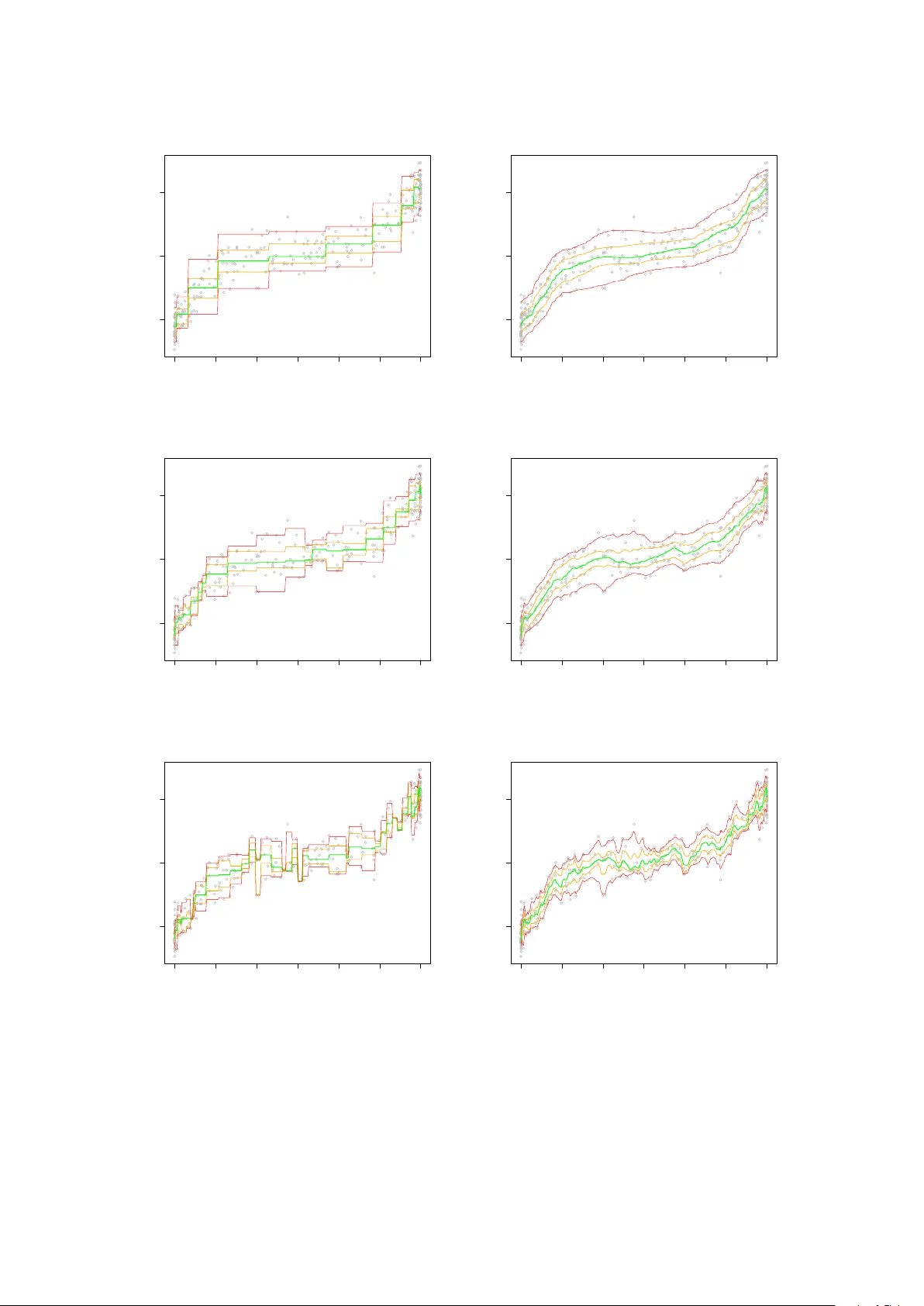
Conditional Quantile Estima tion thr ough Optimal Quantiza tion Isabelle Charlier (1 , 2 , 3) ∗ D a vy P aind a veine (1 , 2) † Jér ôme Saracco (3) July 1, 2021 (1) Université Libr e de Bruxel les, Dép artement de Mathématique, Boulevar d du T riomphe, Campus Plaine, CP210, B-1050, Bruxel les, Belgique. ischarli@ulb.ac.be , dpaindav@ulb.ac.be (2) ECARES, 50 A venue F.D. R o osevelt, CP114/04, B-1050, Bruxel les, Belgique. (3) Université de Bor de aux, Institut de Mathématiques de Bor de aux, UMR CNRS 5251 et INRIA Bor de aux Sud-Ouest, é quip e CQFD, 351 Cours de la Lib ér ation, 33405 T alenc e. Jerome.Saracco@math.u- bordeaux1.fr Abstract In this pap er, w e use quantization to construct a nonparametric estimator of conditional quan tiles of a scalar response Y giv en a d -dimensional v ector of co v ariates X . First we fo cus on the population lev el and show ho w optimal quantization of X , whic h consists in discretiz- ing X b y pro jecting it on an appropriate grid of N p oin ts, allo ws to approximate conditional quan tiles of Y given X . W e sho w that this is appro ximation is arbitrarily go od as N goes to infinit y and provide a rate of conv ergence for the appro ximation error. Then w e turn to the sample case and define an estimator of conditional quantiles based on quantization ideas. W e pro ve that this estimator is consisten t for its fixed- N p opulation counterpart. The results are illustrated on a n umerical example. Dominance of our estimators ov er lo cal con- stan t/linear ones and nearest neighbor ones is demonstrated through extensive sim ulations in the companion paper Charlier et al. ( 2014 ). ∗ Researc h is supported by a Bourse F.R.I.A. of the F onds National de la Recherc he Scien tifique, Comm unauté française de Belgique. † Researc h is supported by an A.R.C. con tract from the Communauté F rançaise de Belgique and by the IAP researc h net work grant P7/06 of the Belgian gov ernment (Belgian Science P olicy). 1 1 In tro duction In numerous applications, one considers regression mo delling to assess the impact of a d - dimensional v ector of cov ariates X on a scalar resp onse v ariable Y . It is then classical to consider the conditional mean and v ariance functions x 7→ E[ Y | X = x ] and x 7→ V ar[ Y | X = x ] , (1.1) resp ectiv ely . A muc h more thorough picture, ho wev er, is obtained b y considering, for v arious α ∈ (0 , 1) , the conditional quan tile functions x 7→ q α ( x ) = inf  y ∈ R : F ( y | x ) ≥ α  , (1.2) where F ( · | x ) denotes the conditional distribution of Y giv en X = x . These conditional quantile functions completely characterize the conditional distribution of Y giv en X , whereas ( 1.1 ), in con trast, only measures the impact of X on Y ’s lo cation and scale, hence ma y completely miss to capture a p ossible impact of X on the shap e of Y ’s distribution, for instance. An imp ortan t application of conditional quantiles is that they provide reference curv es or surfaces (the graphs of x 7→ q α ( x ) for v arious α ) and conditional prediction interv als (in terv als of the form I α ( x ) = [ q α ( x ) , q 1 − α ( x )] , for fixed x ) that are widely used in many differen t areas. In medicine, reference gro wth curv es for c hildren’s height and weigh t as a function of age are considered. Reference curves are also of high interest in economics (e.g., to study discrimination effects and trends in income inequality), in ecology (to observe how some co v ariates can affect limiting sustainable p opulation size), and in lifetime analysis (to assess influence of risk factors on surviv al curves), among many others. Quan tile regression, that concerns the estimation of conditional quantile curves, w as in tro- duced in the seminal pap er Koenker and Bassett ( 1978 ), where the fo cus w as on linear regression. Since then, there has b een m uch researc h on quan tile regression, in particular in the nonpara- metric regression framework. Kernel and nearest-neighbor estimators of conditional quan tiles w ere in vestigated in Bhattachary a and Gangopadh ya y ( 1990 ), while Y u and Jones ( 1998 ) fo cused on local linear quan tile regression and double-kernel approac hes. Many other estimators w ere also considered; see, among others, F an et al. ( 1994 ), Gannoun et al. ( 2002 ), Heagert y and Pepe ( 1999 ), or Y u et al. ( 2003 ). In this work, w e introduce a new nonparametric regression quantile metho d, based on optimal quantization . Optimal quantization is a to ol that w as first used b y engineers in signal and information the- ory , where “quan tization” refers to the discretization of a contin uous signal using a finite n umber of points, called quantizers . The aim b eing to ac hieve an efficien t, parsimonious, transmission of the signal, the num b er and location of the quantizers hav e to b e optimized. Quantization was 2 later used in cluster analysis, pattern and sp eec h recognition. More recently , it w as considered in probabilit y theory; see, e.g., Zador ( 1964 ) or Pagès ( 1998 ). In this con text, the problem of optimal quantization consists in finding the b est approxima tion of a contin uous d -dimensional probabilit y distribution P by a discrete probability distribution charging a fixed num b er N of p oin ts. In other w ords, the d -dimensional random v ector X needs to b e approximated b y a random vector e X N that may assume at most N v alues. Quan tization w as extensiv ely in ves- tigated in n umerical probability , finance, stochastic pro cesses, and numerical integration ; see, e.g., P agès et al. ( 2004a ), Pagès et al. ( 2004b ), or Bally et al. ( 2005 ). Quan tization, ho wev er, w as seldom used in statistics. T o the b est of our knowledge, its applications in statistics are restricted to Sliced In v erse Regression ( Azaïs et al. , 2012 ) and clustering ( Fischer , 2010 and Fischer , 2013 ). As announced ab o v e, we use in this pap er quanti- zation in a nonparametric quan tile regression framew ork. In this context, indeed, quantization naturally takes care of the lo calization-in- x required in any nonparametric regression metho d. The resulting quantization-based estimators inheren tly are based on adaptive bandwidths, hence ma y dominate the lo cal constan t and lo cal linear estimators Y u and Jones ( 1998 ) that t ypically in volv e a unique global bandwidth. Quantization-based estimators also pro vide a refinement o ver nearest-neighbor estimators (suc h as those from Bhattachary a and Gangopadhy a y ( 1990 )) since, unlik e the latter, the n umber of “neighbors” the former consider depends on the point x at whic h q α ( x ) is to b e estimated. This dominance o ver these tw o standard comp etitors, in terms of MSEs, is demonstrated through extensiv e sim ulations in the companion pap er Charlier et al. ( 2014 ). The outline of the pap er, that mostly fo cuses on theoretical asp ects, is as follows. Section 2 discusses quantization and pro vides some results on quan tization, both of a theoretical and algo- rithmic nature. Section 3 describ es how to approximate conditional quantiles through optimal quan tization, whic h is achiev ed b y replacing X in the definition of conditional quan tiles b y its L p -optimal quan tized v ersion e X N (for some fixed N ). The conv ergence rate of this appro xima- tion to the true conditional quantiles is obtained. Section 4 defines the corresp onding estimator and pro v es its consistency (for the fixed- N approximated conditional quan tiles). The results are illustrated on a numerical example, in which a smo oth v ariant of the prop osed estimator based on the b ootstrap is also in tro duced. Section 5 pro vides some final comments. Ev en tually , the App endix collects technical pro ofs. 3 2 Optimal quantization In this section, w e define the concept of L p -norm optimal quan tization and state the main results that will b e used in the sequel (Section 2.1 ). Then w e describ e a sto c hastic algorithm that allows to perform optimal quantization (Section 2.2 ), and pro vide some conv ergence results for this algorithm (Section 2.3 ). 2.1 Definition and main results Let X b e a random d -vector defined on a probability space (Ω , F , P ) , with distribution P X , and fix a real num ber p ≥ 1 such that E[ | X | p ] < ∞ (throughout, | · | denotes the Euclidean norm). Quan tization replaces X with an appropriate random d -vector π ( X ) that assumes at most N v alues. In optimal L p -norm quan tization, the v ector π ( X ) minimizes the L p -norm quan tization error k π ( X ) − X k p , with k Z k p :=  E  | Z | p  1 /p . This optimization problem is equiv alen t to finding an N -grid of R d — γ N , say — such that the pro jection e X γ N = Pro j γ N ( X ) of X on the (Euclidean-)nearest p oin t of the grid minimizes the quantization err or k e X γ N − X k p . This definition leads to tw o natural questions: does suc h a minim um alwa ys exist? How do es this minimum b eha ve as N go es to infinity? Existence (but not unicity) of an optimal N -grid — that is, a grid minimizing this quantiza- tion error — has b een obtained under the assumption that P X do es not c harge any h yp erplane; see Pagès ( 1998 ). Irrespective of the sequence of optimal grids considered, e X N con verges to X in L p . This is a direct corollary of the following result, which is often referred to as Zador’s theorem ( Zador , 1964 ) and provides the rate of conv ergence of the quantization error; see, e.g., Graf and Lusc hgy ( 2000 ) for a pro of. Theorem 2.1. Assume that k X k p + δ < ∞ for some δ > 0 . L et P X ( du ) = f ( u ) λ d ( du ) + ν ( du ) b e the L eb esgue de c omp osition of P X , wher e λ d is the L eb esgue me asur e on R d and ν ⊥ λ d . Then lim N →∞  N p d min γ N ∈ ( R d ) N k e X γ N − X k p p  = J p,d  Z R d ( f ( u )) d p + d du  1+ p d , with J p,d = min N  N p/d min γ N ∈ ( R d ) N D p,U N ( γ N )  , wher e D p,U N ( γ N ) denotes the ( p th p ower of the) quantization err or, obtaine d for the uniform distribution over [0 , 1] d , when c onsidering the grid γ N ∈ ( R d ) N . In dimension d = 1 , one has J p,d = 1 2 p ( p +1) . F or d > 1 , little is kno wn ab out J p,d , but it can b e shown that J p,d ∼  d 2 π e  p/ 2 as d → ∞ ; see Graf and Luschgy ( 2000 ). 4 Corollary 2.2. Assume that k X k p + δ < ∞ for some δ > 0 . Then, for some C, D ∈ R and N 0 ∈ N , we have that k e X γ N − X k p p ≤ 1 N p/d  C k X k p + δ p + δ + D  , for al l N ≥ N 0 . Summing up, there exist L p -optimal N -grids — or optimal N -quantizers — that minimize the quantization error. A further natural question then is: ho w to obtain an optimal N -grid? W e no w discuss a sto c hastic algorithm that addresses this problem. 2.2 The sto c hastic gradient algorithm Except in some very exceptional cases (suc h as the uniform ov er a compact interv al of the real line), optimal N -grids hav e no closed form. That is, there exist no results that describ e the geometric structure of such grids. Ho wev er, one can attempt to obtain (approximations of ) optimal N -grids through a sto chastic gr adient algorithm suc h as the following. Let ( ξ t ) t ∈ N 0 , N 0 = { 1 , 2 , . . . } , b e a sequence of indep enden t and identically P X -distributed random v ectors, and let ( δ t ) t ∈ N 0 b e a deterministic sequence in (0 , 1) suc h that ∞ X t =1 δ t = + ∞ and ∞ X t =1 δ 2 t < + ∞ (throughout the pap er, we tacitly assume that the algorithm makes use of a sequence δ t that satisfies these conditions). The algorithm starts from a deterministic N -tuple X 0 = x 0 with N pairwise distinct entries. This initial N -grid x 0 is then up dated as follow s. F or ev ery t ∈ N 0 , define recursiv ely the grid X t as X t = X t − 1 − δ t p ∇ x d p N ( X t − 1 , ξ t ) , (2.1) where ∇ x d p N ( x, ξ ) stands for the gradien t with resp ect to the x -argument of the so-called lo cal quan tization error d p N ( x, ξ ) = min 1 ≤ i ≤ N | x i − ξ | p , with x = ( x 1 , . . . , x N ) ∈ ( R d ) N and ξ ∈ R d . Note that, for any ξ , the i th entry of this gradient is given b y  ∇ x d p N ( x, ξ )  i = p | x i − ξ | p − 1 x i − ξ | x i − ξ | I [ x i = Pro j x ( ξ )] , where I A denotes the indicator function of the set A , and with the con v ention 0 / 0 = 1 when x i = ξ . This implies that the N -v ector ∇ x d p N ( x, ξ ) alwa ys has exactly one non-zero entry , namely the one corresponding to the point of the grid x that is closest to ξ . Consequen tly , at each step t of the algorithm, only one p oin t of the grid X t − 1 will b e changed to define the grid X t , namely the p oin t from the grid X t − 1 that is closest to ξ t . 5 More details ab out this algorithm can b e found in P agès and Printems ( 2003 ). F or p = 2 , this is known as the Comp etitive L e arning V e ctor Quantization (CL V Q) algorithm, and is the most commonly used one in quantization. This success is explained by the fact that the con vergence results obtained for the CL VQ algorithm are muc h more satisfactory than for p 6 = 2 . 2.3 Con v ergence results for the CL V Q algorithm Here we state sev eral results sho wing that the grids pro vided by the CL V Q algorithm conv erge to optimal grids as the num ber of iterations t go es to infinity . W e start with the univ ariate case ( d = 1 ). Assume that the supp ort of P X is compact and let its conv ex hull C b e [ a, b ] . W rite F + N := { x = ( x 1 , . . . , x N ) : a < x 1 < · · · < x N < b } for the set of N -grids on C inv olving pairwise distinct p oin ts stored in ascending order, and let ¯ F + N b e its closure; see P agès ( 1998 ). Denote by D 2 ,P X N ( x ) = R C min 1 ≤ i ≤ N | x i − w | 2 P X ( dw ) the (squared) L 2 -norm quan tization error asso ciated with a giv en grid x = ( x 1 , . . . , x N ) ∈ F + N . Theorem 2.3 ( Pagès , 1998 , Th. 27) . In the univariate setup ab ove, we have the fol lowing. (i) Assume that P X is absolutely c ontinuous with a density f : [ a, b ] → R + that is p ositive on ( a, b ) , and assume either that f is strictly lo g-c onc ave or that it is lo g-c onc ave with f ( a +) − f ( b − ) > 0 . Then x 7→ D 2 ,P X N ( x ) has a unique minimizer x ∗ in ¯ F + N , which c oincides with the unique solution of ∇ D 2 ,P X N ( x ) = 0 in ¯ F + N (when P X is the uniform over [0 , 1] , the optimal grid is x ∗ =  a + 2 k − 1 2 N ( b − a )  1 ≤ k ≤ N ) . (ii) Irr esp e ctive of the initial grid X 0 ∈ F + N , every tr aje ctory ( X 0 , X 1 , X 2 , . . . ) of the CL VQ algorithm is a.s. such that X t ∈ F + N for al l t . If P X is absolutely c ontinuous and if ther e ar e finitely many grids x ( ∈ ¯ F + N ) such that ∇ D 2 ,P X N ( x ) = 0 , then X t a.s − − → x ∗ as t → ∞ , with ∇ D 2 ,P X N ( x ∗ ) = 0 . P art (i) of the result provide s a particular family of distributions for which the optimal grid is unique (recall that existence alw ays holds). Bey ond stating that tra jectories of the CL VQ algorithm live in F + N (with grids that therefore stays of size N ), Part (ii) of the result provides mild conditions under whic h the algorithm almost surely provides a limiting grid that is a critical p oin t of the quan tization error, hence, under the assumptions of Part (i), is optimal. Unfortunately , the picture is less clear for the multiv ariate case ( d > 1 ). While it is still so that the grid X t will hav e pairwise distinct comp onen ts for an y t , some of the comp onen ts of the limiting grid x ∗ , if an y , may coincide. (a) If, parallel to the univ ariate case, this do es not happ en, then the a.s. conv ergence of X t to a critical point of the quan tization error D 2 ,P X N ( · ) can b e established under the assumption 6 that P X has a b ounded density with a compact and conv ex supp ort. (b) Otherwise, no conv ergence results are av ailable; the only optimality results that can then b e obtained relate to appro ximations in volving grids of size k < N , where k is the n umber of distinct components in the limiting grid x ∗ , which is quite differen t from the original N -quan tization problem considered initially . The in terested reader may refer to P agès ( 1998 ) for details. F or practical purp oses, though, one should not w orry to m uch, as all n umerical exercices w e conducted w ere compatible with case (a) (with increasing t , the smallest distance b et ween tw o comp onen ts of X t alw ays seemed to stabilize rather than decreasing to zero). 3 Conditional quantiles through optimal quan tization Let us come bac k to the regression setup inv olving a scalar resp onse Y and a d -dimensional vector of cov ariates X , and consider the conditional quan tile functions q α ( · ) in ( 1.2 ). It is well-kno wn that q α ( x ) = arg min a ∈ R E  ρ α ( Y − a ) | X = x  , (3.1) where z 7→ ρ α ( z ) = − (1 − α ) z I [ z < 0] + αz I [ z ≥ 0] = z  α − I [ z < 0]  is the so-called che ck function . As w e now explain, this allows to use optimal quantization to approximate conditional quantiles. T o do so, fix p ≥ 1 suc h that k X k p < ∞ . Then, for any p ositiv e integer N , one may consider the appro ximation e q N α ( x ) = arg min a ∈ R E  ρ α ( Y − a ) | e X N = ˜ x  , (3.2) where e X N and ˜ x are the pro jections of X and x resp ectiv ely onto an L p -optimal N -grid. Since e X N − X go es to zero as N → ∞ , one may expect that e q N α ( x ) pro vides a b etter and b etter appro ximation of q α ( x ) as N increases. The main goal of this section is to quantify the quality of this appro ximation. W e will need the follo wing assumptions. Assumption (A) (i) The random v ector ( X , Y ) is generated through Y = m ( X , ε ) , where the d -dimensional co v ariate v ector X and the error ε are mutually indep enden t; (ii) the link function ( x, z ) 7→ m ( x, z ) is of the form m 1 ( x ) + m 2 ( x ) z , where the functions m 1 ( · ) : R d → R and m 2 ( · ) : R d → R + 0 are Lipschitz functions; (iii) k X k p < ∞ and k ε k p < ∞ ; (iv) the distribution of X do es not charge any hyperplane. Note that Assumption (A)(ii)-(iii) directly implies that there exists C > 0 suc h that the link 7 function m ( · , ε ) of the mo del ab o v e satisfies ∀ u, v ∈ R d , k m ( u, ε ) − m ( v , ε ) k p ≤ C | u − v | . (3.3) The resulting Lipsc hitz constant — that is, the smallest real n umber C for which ( 3.3 ) holds — is [ m ] Lip = [ m 1 ] Lip + [ m 2 ] Lip k ε k p , where [ m 1 ] Lip and [ m 2 ] Lip are the corresp onding Lipschitz constan ts of m 1 and m 2 , resp ectiv ely . Assumption (B) (i) The support S X of P X is compact; (ii) ε admits a con tinuous den- sit y f ε : R → R + 0 (with resp ect to the Leb esgue measure on R ). T o obtain rates of con vergence, we will need the follo wing reinforcemen t of Assumption (A). Assumption (A 0 ) Same as Assumption (A), but with (iii) replaced by (iii) 0 there exists δ > 0 such that k X k p + δ < ∞ , and k ε k p < ∞ . W e can then pro ve the following result (see the App endix for the pro of ). Theorem 3.1. Fix α ∈ (0 , 1) . Then (i) under Assumptions (A)-(B), k e q N α ( X ) − q α ( X ) k p ≤ 2 r max  α 1 − α , 1 − α α  [ m ] 1 / 2 Lip   L N ( X )   1 / 2 p k X − e X N k 1 / 2 p , for N sufficiently lar ge, wher e ( L N ( X )) is a se quenc e of X -me asur able r andom variables that is b ounde d in L p ; (ii) under Assumptions (A 0 )-(B), k e q N α ( X ) − q α ( X ) k p = O ( N − 1 / 2 d ) , as N → ∞ . Of course, fixed- x consistency results are also quite app ealing in quan tile regression. Such a result is pro vided in the following theorem (see the App endix for the pro of ). Theorem 3.2. Fix α ∈ (0 , 1) . Then, under Assumptions (A)-(B), sup x ∈ S X   e q N α ( x ) − q α ( x )   → 0 , as N → ∞ . Unlik e in Theorem 3.1 , Theorem 3.2 do es not pro vide any rate of con vergence. This is a consequence of the fact that, while the conv ergence of e X N to wards X can be sho wn to imply the conv ergence of ˜ x to w ards x for eac h fixed x , it do es not seem p ossible to show that the rate of con vergence in the fixed- x conv ergence is inherited from the conv ergence inv olving X . 8 4 Quan tized conditional quan tile estimators 4.1 The prop osed estimators and their consistency Consider now the problem of estimating the conditional quantile q α ( x ) on the basis of indep en- den t copies ( X 1 , Y 1 ) , . . . , ( X n , Y n ) of ( X, Y ) . F or any N ( < n ) , the appro ximation e q N α ( x ) in ( 3.2 ) leads to an estimator b q N ,n α ( x ) of the conditional quan tile q α ( x ) , through the following t wo steps : (S1) First, the CL VQ algorithm from Section 2.2 is applied to p erform quantization in X . F or this purpose, (i) the initial grid X 0 is obtained b y sampling randomly among the X i ’s without replacemen t, and with the constrain t 1 that the same x -v alues cannot b e pick ed more than once; (ii) n iterations are p erformed, based on ξ t = X t , t = 1 , . . . , n . W e write ˆ γ N ,n = ( ˆ x N ,n 1 , . . . , ˆ x N ,n N ) for the resulting grid and b X N ,n = Pro j ˆ γ N ,n ( X ) for the corresp onding (empirical) quan tization of X ; to mak e the notation less heavy , w e will stress dep endence on n in these quantities only when it is necessary . (S2) Second, the approximation e q N α ( x ) = arg min a E[ ρ α ( Y − a ) | e X N = ˜ x ] is then estimated by b q N ,n α ( x ) = arg min a P n i =1 ρ α ( Y i − a ) I [ b X N i = ˆ x N ] , where b X N i = b X N ,n i = Pro j ˆ γ N ,n ( X i ) and ˆ x N = ˆ x N ,n = Pro j ˆ γ N ,n ( x ) . Of course, b q N ,n α ( x ) , in practice, is simply ev aluated as the sample α -quan tile of the Y i ’s whose corresp onding b X N i is equal to ˆ x N . Note that the num b er of iterations is equal to the sample size n at hand, so that it is exp ected that only mo derate-to-large n will provide reasonable approximations of optimal N -grids. F or fixed N (and x ), the con vergence in probability of b q N ,n α ( x ) to e q N α ( x ) as n → ∞ can be obtained by making use of the conv ergence results for the stochastic gradient algorithm discussed in Section 2 . In order to do so, w e need to restrict to p = 2 (that is, to the CL V Q algorithm) and to adopt the following assumption. Assumption (C) P X is absolutely con tinuous with resp ect to the Leb esgue measure on R d . W e then ha ve the following result. Theorem 4.1. Fix α ∈ (0 , 1) , x ∈ S X and N ∈ N 0 . Then, under Assumptions (A), (B)(i), and (C), we have that, as n → ∞ , | b q N ,n α ( x ) − e q N α ( x ) | → 0 , 1 If the X i ’s are i.i.d. with a common densit y f , sampling without replacemen t among the X i ’s of course implies that this constrain t will be met with probability one. One often needs to imp ose it, how ev er, in real-data examples (due to the p ossible presence of ties) or when p erforming bo otstrap (see later). 9 in pr ob ability, pr ovide d that quantization is b ase d on p = 2 . In the previous section, we show ed that, as N → ∞ , e q N α ( x ) − q α ( x ) go es to zero almost surely , hence in probabilit y . Theorem 4.1 then suggests that b q N ,n α ( x ) − q α ( x ) might go to zero in probabilit y as b oth n and N go to infinity in some appropriate w a y . Obtaining suc h a double asymptotic results, how ever, is extremely delicate, since, to the b est of our kno wledge, all conv ergence results for the sto c hastic gradient algorithm in the literature are as n → ∞ with N fixed. 4.2 Numerical example and b o otstrap mo dification F or the sak e of illustration, we ev aluated the estimator b q N ,n α ( x ) for N = 10 , 25 , and 40 , in a sample of n = 300 mutually indep enden t observ ations ( X i , Y i ) obtained from the mo del Y = 1 5 X 3 + ε, (4.1) where X = 6 Z − 3 , with Z ∼ Beta(0 . 3 , 0 . 3) , and ε ∼ N (0 , 1) are indep enden t. The left panels in Figure 1 plot the corresponding quan tiles curv es x 7→ b q N ,n α ( x ) for α = 0 . 05 , 0 . 25 , 0 . 5 , 0 . 75 , and 0 . 95 (actually , these curves were ev aluated only at 300 equispaced p oin ts in ( − 3 , 3) ). It is seen that the n um b er of quan tizers N used has an important impact on the curves. F or small N , the curv es are not smooth and show a large bias. F or large N , bias is smaller but the v ariability is large. One should k eep in mind that, for large N , the grid provided by the CL V Q algorithm p oorly approximates the corresponding optimal N -grid, since a fixed num ber n of iterations are used in the algorithm (that should not b e to o small compared to N ). Smo other quan tile curves can b e obtained from the b ootstrap, through the following pro ce- dure. F or some integer B , we first generate grids ˆ γ N ,n b , b = 1 , . . . , B (eac h of size N ), as follows from the CL VQ algorithm: first, we sample N observ ations with replacement from the initial sample X 1 , . . . , X n to generate an initial grid X 0 b (with the same constrain t as in (S1) ab o ve that the N v alues obtained are pairwise differen t); second, we p erform iterations based on ξ t b , t = 1 , . . . , n , that are similarly obtained b y sampling with replacemen t from X 1 , . . . , X n (this time, without an y constraint). This allows to consider the b ootstrap estimators ¯ q N ,n α,B ( x ) = 1 B B X b =1 ˆ q ( b ) α ( x ) , where ˆ q ( b ) α ( x ) = ˆ q ( b ) ,N ,n α ( x ) is obtained b y performing (S2) based on the original sample ( X i , Y i ) , i = 1 , . . . , n , and the grid ˆ γ N ,n b . Bo otstrapping, thus, fo cuses on the construction of the grids. The righ t panels of Figure 1 plot the resulting b ootstrapp ed quan tile curves x 7→ ¯ q N ,n α,B ( x ) for the same v alues of α and N as in the original (non-b o otstrapped) versions. Bo otstrapping 10 clearly smo oths all curves, and moreov er significan tly reduces b oundary effects for small N . These adv an tages require to tak e B large enough. But of course, very large v alues of B should b e av oided in order to k eep the computational burden under control. The main comp etitors to the prop osed quantization-based estimators are the nearest-neigh b or estimators (as those of Bhattachary a and Gangopadh ya y , 1990 ) and the local constan t and local linear estimators from Y u and Jones ( 1998 ). F or the sak e of comparison, w e plot those com- p etitors in Figure 2 , join tly with our bo otstrapp ed estimator (based on B = 50 ), on the same sample used in Figure 1 . F or each estimator, the smo othing parameters in volv ed were selected in an automatic wa y . F or nearest-neigh b or estimators, the n umber k of neighbors to consider w as chosen to minimize the MSE MSE( k ) = 1 N x N x X i =1  b q k α ( x i ) − q α ( x i )  2 , where b q k α ( x ) denotes the nearest-neighbor estima of q α ( x ) based on k neigh b ors and { x 1 , . . . , , x N x } is an equispaced grid on ( − 3 , 3) (note that this metho d uses the p opulation conditional quantiles, hence is infeasible in practice). Local constant/linear estimators (that are based on the Gaussian k ernel) inv olv e a bandwidth that, for fixed α , is selected (here in a gen uinely data-driven wa y) as h α = α (1 − α ) h mean φ (Φ − 1 ( α )) 2 , where φ and Φ are respectively the standard normal densit y and distribution functions. Here, h mean corresp onds to the optimal bandwidth for regression mean estimation and is c hosen through cross-v alidation; see Y u and Jones ( 1998 ). As for the quantization-based estimators, the n umber of quantizers N is selected through a data-driv en metho d that is defined and in vestigated in the companion pap er Charlier et al. ( 2014 ). Since Z is generated according to a beta distribution with (equal) parameter v alues that are smaller than one, the X i ’s are less dense in the middle of the in terv al (-3,3) than close to its b oundaries. The lo cal constant and linear estimators seem to suffer from this fact, as the corresp onding quantiles curves are significan tly less smooth in the middle than at the b oundaries. The nearest-neighbor estimator and our quantization-based estimator provide b etter estimations in the middle part, with an adv antage for our estimator that app ears to b e smo other (despite the fact that, unlik e for the nearest-neighbor estimator, the corresp onding smo othing parameter v alue is chosen in a totally data-driven wa y). 11 −3 −2 −1 0 1 2 3 −5 0 5 X Y −3 −2 −1 0 1 2 3 −5 0 5 X Y −3 −2 −1 0 1 2 3 −5 0 5 X Y −3 −2 −1 0 1 2 3 −5 0 5 X Y −3 −2 −1 0 1 2 3 −5 0 5 X Y −3 −2 −1 0 1 2 3 −5 0 5 X Y Figure 1: Estimated conditional quan tiles curv es x 7→ b q N ,n α ( x ) (left) and their bo otstrapped coun terparts x 7→ ¯ q N ,n α,B ( x ) for B = 50 (righ t), based on N = 10 (top), N = 25 (middle), and N = 50 (b ottom). The sample size is n = 300 , and the quan tiles lev els considered are α =0.05, 0.25, 0.5, 0.75, and 0.95. See ( 4.1 ) for the data generating mo del. 12 −3 −2 −1 0 1 2 3 −5 0 5 X Y −3 −2 −1 0 1 2 3 −5 0 5 X Y −3 −2 −1 0 1 2 3 −5 0 5 X Y −3 −2 −1 0 1 2 3 −5 0 5 X Y Figure 2: The prop osed estimated conditional quantiles curves x 7→ ¯ q N ,n α,B ( x ) for B = 50 (top left), their nearest- neigh b or comp etitors from Bhattac harya and Gangopadh ya y ( 1990 ) (top righ t), and their lo cal constan t and lo cal linear comp etitors from Y u and Jones ( 1998 ) (bottom left and b ottom righ t, resp ectiv ely). The sample is the same as in Figure 1 . 13 5 Final comments In this pap er, we presented a new method to estimate nonparametrically conditional quantile curv es of Y giv en X . The main idea is to use optimal quantization as an alternative to more standard lo calization techniques such as kernel or nearest-neighbor metho ds. Our construction consists in replacing X in the definition of conditional quantiles with a quantized v ersion of X . W e show ed that this pro vides a v alid approximation of conditional quan tiles. In the empirical case, this appro ximation leads to new estimators of conditional quan tiles, that, as we pro v ed, are (for fixed N ) consistent to their p opulation counterparts. W e illustrated the b eha vior of these estimators on a n umerical example, and show ed that N essen tially b eha ves as a smo othing parameter, parallel to the bandwidth and the n umber of neigh b ors to be used for kernel and nearest-neighbor methods, resp ectiv ely . Of course, extensiv e sim ulations are needed to compare the performances of the prop osed estimators with these classical competitors. This is achiev ed in the companion pap er Charlier et al. ( 2014 ), where it is sho wn that quan tization-based estimators tend to dominate their comp etitors in terms of MSEs as so on as X is not uniformly distributed. There, a metho d to choose empirically the smoothing parameter N is also developed and inv estigated. A Pro ofs of Section 3 In this section, we pro ve Theorems 3.1 and 3.2 , which requires to establish several lemmas. W e first introduce some notation. Let G a ( x ) = E[ ρ α ( Y − a ) | X = x ] and denote the corresp onding quan tized quan tity by e G a ( ˜ x ) = E[ ρ α ( Y − a ) | e X N = ˜ x ] . Since e q = e q N α ( x ) = arg min a ∈ R e G a ( ˜ x ) and q = q α ( x ) = arg min a ∈ R G a ( x ) , it is natural to try to control the distance b et ween e G a ( ˜ x ) and G a ( x ) . This is ac hieved in Lemma A.2 , the pro of of whic h requires the follo wing preliminary result. Lemma A.1. Fix α ∈ (0 , 1) and a ∈ R . Then, under Assumption (A), (i) ρ α : R → R is Lipschitz, with Lipschitz c onstant [ ρ α ] Lip = max( α , 1 − α ) , and (ii) G a : R d → R is Lipschitz, with Lipschitz c onstant [ G a ] Lip = max( α, 1 − α )[ m ] Lip . Pr o of of L emma A.1 . Since (i) is a trivial calculus exercise, w e only pro ve (ii). T o do so, note that, for an y u, v ∈ R d , | G a ( u ) − G a ( v ) | =   E[ ρ α ( Y − a ) | X = u ] − E[ ρ α ( Y − a ) | X = v ]   =   E[ ρ α ( m ( X , ε ) − a ) | X = u ] − E[ ρ α ( m ( X , ε ) − a ) | X = v ] | , 14 so that the indep endence of X and ε entails | G a ( u ) − G a ( v ) | ≤ E[ | ρ α ( m ( u, ε ) − a ) − ρ α ( m ( v , ε ) − a ) | ] ≤ [ ρ α ] Lip [ m ] Lip | u − v | , where the last inequalit y follows from Part (i) of the result and equation ( 3.3 ). W e still need the follo wing lemma to pro ve Theorem 3.2 . Lemma A.2. Fix α ∈ (0 , 1) and x ∈ S X . F or any inte ger N , let ˜ x = ˜ x N = Pro j γ N ( x ) and C x = C N x = { z ∈ S X : Pro j γ N ( z ) = ˜ x } . Then, under Assumptions (A)-(B), (i) sup x ∈ S X | x − ˜ x | → 0 as N → ∞ ; (ii) sup x ∈ S X R ( C x ) → 0 as N → ∞ , wher e we let R ( C x ) := sup z ∈ C x | z − ˜ x | ; (iii) sup x ∈ S X sup a ∈ R | e G a ( ˜ x ) − G a ( x ) | → 0 as N → ∞ ; (iv) sup x ∈ S X | min a ∈ R e G a ( ˜ x ) − min a ∈ R G a ( x ) | → 0 as N → ∞ . Pr o of of L emma A.2 . (i) Assume by con tradiction that there exists ε > 0 such that, for infinitely man y N (for N ∈ N ( ε ) , sa y), w e hav e sup x ∈ S X | ˜ x N − x | > ε . F or any suc h v alue of N , one can pick x ∈ S X (that may dep end on N ) with | ˜ x N − x | > ε . No p oin t of the optimal grid γ N b elongs to the ball B ( x, ε ) = { z ∈ R d : | z − x | < ε } , whic h implies that, for all z ∈ B ( x, ε/ 2) , | ˜ z N − z | > ε/ 2 , where ˜ z is the pro jection of z onto γ N . Therefore, for N ∈ N ( ε ) , k X γ N − X k p p = Z Supp ( P X ) | ˜ z N − z | p dP X ( z ) ≥ Z B ( x,ε/ 2) | ˜ z N − z | p dP X ( z ) >  ε 2  p inf y ∈ S X P X  B ( y, ε/ 2)  =: δ ε > 0 , (A.1) where the last inequality follows from the fact that y 7→ P X  B ( y, ε/ 2)  is a contin uous function taking only strictly p ositiv e v alues on the compact set S X . Since the cardinalit y of N ( ε ) is infinite, ( A.1 ) prev ents k X γ N − X k p to go to zero as N → ∞ , a contradiction. (ii) Since S X is compact, w e hav e that, for an y x , the radius of the quan tization cell C x is b ounded. Hence, for any x , there exists x ∗ N ∈ C x suc h that R ( C x ) = sup z ∈ C x | z − ˜ x | = | x ∗ N − ˜ x | ≤ sup x ∈ S X | x − ˜ x | . Hence, sup x ∈ S X R ( C x ) ≤ sup x ∈ S X | x − ˜ x | . The result then follo ws from Part (i). (iii) Fix a ∈ R . First note that, since [ e X N = ˜ x ] is equiv alen t to [ X ∈ C x ] , one has | E[ ρ α ( Y − a ) | e X N = ˜ x ] − E[ ρ α ( Y − a ) | X = ˜ x ] | ≤ sup z ∈ C x | E[ ρ α ( Y − a ) | X = z ] − E[ ρ α ( Y − a ) | X = ˜ x ] | . 15 Therefore, | e G a ( ˜ x ) − G a ( x ) | = | E[ ρ α ( Y − a ) | e X N = ˜ x ] − E[ ρ α ( Y − a ) | X = x ] | ≤ | E[ ρ α ( Y − a ) | e X N = ˜ x ] − E[ ρ α ( Y − a ) | X = ˜ x ] | + | E[ ρ α ( Y − a ) | X = ˜ x ] − E[ ρ α ( Y − a ) | X = x ] | ≤ 2 sup z ∈ C x | E[ ρ α ( Y − a ) | X = z ] − E[ ρ α ( Y − a ) | X = ˜ x ] | . Using the indep endence b et ween X and ε and the Lipsc hitz prop erties of ρ α and m then yields | e G a ( ˜ x ) − G a ( x ) | ≤ 2 sup z ∈ C x | E[ ρ α ( m ( z , ε ) − a ) − E[ ρ α ( m ( ˜ x, ε ) − a )] | ≤ 2 max( α, 1 − α )[ m ] Lip sup z ∈ C x | z − ˜ x | = 2 max( α, 1 − α )[ m ] Lip R ( C x ) . (A.2) Hence, sup x ∈ S X sup a ∈ R | e G a ( ˜ x ) − G a ( x ) | ≤ 2 max( α, 1 − α )[ m ] Lip sup x ∈ S X R ( C x ) . The results then follo ws from Part (ii). (iv) Letting I + = I [min a ∈ R e G a ( ˜ x ) ≥ min a ∈ R G a ( x )] , w e hav e | min a ∈ R e G a ( ˜ x ) − min a ∈ R G a ( x ) | I + =  e G e q N α ( x ) ( ˜ x ) − G q α ( x ) ( x )  I + ≤  e G q α ( x ) ( ˜ x ) − G q α ( x ) ( x )  ) I + ≤ sup a ∈ R | e G a ( ˜ x ) − G a ( x ) | I + . Pro ceeding similarly with I − = I [min a ∈ R e G a ( ˜ x ) < min a ∈ R G a ( x )] , this yields | min a ∈ R e G a ( ˜ x ) − min a ∈ R G a ( x ) | I − =  G q α ( x ) ( x ) − e G e q N α ( x ) ( ˜ x )  I − ≤  G e q N α ( x ) ( x ) − e G e q N α ( x ) ( ˜ x )  I − ≤ sup a ∈ R | e G a ( ˜ x ) − G a ( x ) | I − , so that | min a ∈ R e G a ( ˜ x ) − min a ∈ R G a ( x ) | ≤ sup a ∈ R | e G a ( ˜ x ) − G a ( x ) | . The result therefore follows from P art (iii). W e can no w prov e Theorem 3.2 . Pr o of of The or em 3.2 . First note that, for any x ∈ S X , | G e q N α ( x ) ( x ) − G q α ( x ) ( x ) | ≤ | G e q N α ( x ) ( x ) − e G e q N α ( x ) ( ˜ x ) | + | e G e q N α ( x ) ( ˜ x ) − G q α ( x ) ( x ) | ≤ sup a ∈ R | G a ( x ) − e G a ( ˜ x ) | + | min a ∈ R e G a ( ˜ x ) − min a ∈ R G a ( x ) | ≤ sup x ∈ S X sup a ∈ R | G a ( x ) − e G a ( ˜ x ) | + sup x ∈ S X | min a ∈ R e G a ( ˜ x ) − min a ∈ R G a ( x ) | . 16 Therefore, Lemma A.2 (iii)-(iv) readily implies that, as N → ∞ , sup x ∈ S X | G e q N α ( x ) ( x ) − G q α ( x ) ( x ) | → 0 . (A.3) No w, let ˜ N be suc h that, for any N ≥ ˜ N , w e hav e | G e q N α ( x ) ( x ) − G q α ( x ) ( x ) | ≤ 1 for all x ∈ S X . As w e will show later in this pro of, this implies that there exists M such that | e q N α ( x ) − q α ( x ) | ≤ M , (A.4) for all x ∈ S X and N ≥ ˜ N . One can easily chec k that, for any x ∈ S X , a 7→ G a ( x ) is twice contin uously differentiable, with deriv ativ es dG a ( x ) da = F ε  a − m 1 ( x ) m 2 ( x )  − α and d 2 G a ( x ) da 2 = 1 m 2 ( x ) f ε  a − m 1 ( x ) m 2 ( x )  . Consequen tly , p erforming a second-order expansion ab out a = q α ( x ) pro vides G e q N α ( x ) ( x ) − G q α ( x ) ( x ) = 1 m 2 ( x ) f ε  q N α ∗ ( x ) − m 1 ( x ) m 2 ( x )  ( e q N α ( x ) − q α ( x )) 2 , for some q N α ∗ ( x ) b et w een e q N α ( x ) and q α ( x ) . Therefore, sup x ∈ S X ( e q N α ( x ) − q α ( x )) 2 ≤ sup x ∈ S X m 2 ( x ) inf x ∈ S X f ε  q N α ∗ ( x ) − m 1 ( x ) m 2 ( x )  sup x ∈ S X | G e q N α ( x ) ( x ) − G q α ( x ) ( x ) | . (A.5) Since m 2 ( · ) is a con tinuous function defined ov er the compact set S X , w e hav e sup x ∈ S X m 2 ( x ) ≤ C a (A.6) for some constan t C a . Using ( A.4 ) and the fact that q α ( · ) , m 1 ( · ) , and m 2 ( · ) are con tin uous functions also defined ov er this compact set (with m 2 ( · ) taking strictly p ositiv e v alues), we hav e that, for N ≥ ˜ N , sup x ∈ S X | q N α ∗ ( x ) − m 1 ( x ) | m 2 ( x ) ≤ sup x ∈ S X  | q α ( x ) | + | m 1 ( x ) | + M  inf x ∈ S X m 2 ( x ) ≤ C b , for some constant C b . Jointly with the contin uity of the p ositiv e function f ε ( · ) , this implies that the infimum in ( A.5 ) admits a strictly p ositiv e lo wer b ound that is indep enden t of N (for N ≥ ˜ N ). Using this, ( A.3 ) and ( A.6 ), we conclude from ( A.5 ) that sup x ∈ S X ( e q N α ( x ) − q α ( x )) 2 → 0 , as N → ∞ , whic h was to b e pro ved. It remains to sho w that the claim in ( A.4 ) indeed holds true. By con tradiction, assume that for all M , there exists x = x M (and N ≥ ˜ N ) suc h that | e q N α ( x ) − q α ( x ) | > M . The con v exity 17 of a 7→ G a ( x ) and the fact that | G e q N α ( x ) ( x ) − G q α ( x ) ( x ) | ≤ 1 for all x ∈ S X (for N ≥ ˜ N ) readily implies that, for an y a with | a − q α ( x ) | ≤ M , G a ( x ) ≤ G q α ( x ) ( x ) + | a − q α ( x ) | M . Since this holds for all arbitrarily large M , the conv exity of G a ( x ) implies that f ε  q α ( x ) + 1 − m 1 ( x ) m 2 ( x )  = d 2 G a ( x ) da 2      a = q α ( x )+1 → 0 as M → ∞ . The same argumen t as ab o v e, how ev er, sho ws that inf x ∈ S X f ε  q α ( x )+1 − m 1 ( x ) m 2 ( x )  > 0 , a con tradiction. The pro of of Theorem 3.1 requires the following three lemmas. Lemma A.3. Fix α ∈ (0 , 1) . Then (i) under Assumptions (A)-(B), we have   sup a   e G a ( e X N ) − G a ( X )     p ≤ 2 max( α, 1 − α )[ m ] Lip   e X N − X   p ; (A.7) (ii) under Assumptions (A 0 )-(B), we have that   sup a   e G a ( e X N ) − G a ( X )     p = O  N − 1 /d  , as N → ∞ . Lemma A.4. Fix α ∈ (0 , 1) . Then (i) under Assumptions (A)-(B), we have   e G ˜ q ( e X N ) − G q ( X )   p ≤ 2 max( α, 1 − α )[ m ] Lip   e X N − X   p ; (ii) under Assumptions (A 0 )-(B),   e G ˜ q ( e X N ) − G q ( X )   p = O ( N − 1 /d ) as N → ∞ . Lemma A.5. L et Assumption (B) hold. F or any x ∈ S X , let L ( x ) = 1 /f Y | X = x ( q α ( x )) and L N ( x ) = 1 /f Y | X = x ( c N ( x )) , wher e c N ( x ) is the infimum of al l c ’s b etwe en ˜ q N α ( x ) and q α ( x ) for which Z max( q α ( x ) , ˜ q N α ( x )) min( q α ( x ) , ˜ q N α ( x )) f Y | X = x ( y ) dy = f Y | X = x ( c ) | ˜ q N α ( x ) − q α ( x ) | (A.8) (existenc e fol lows fr om the me an value the or em). Then k L N ( X ) k p → k L ( X ) k p as N → ∞ . Pr o of of L emma A.3 . P art (ii) of the result readily follows from Part (i) and Corollary 2.2 , so that we may fo cus on the pro of of P art (i). Note that G a ( e X N ) stands for the conditional 18 exp ectation of ρ α ( Y − a ) giv en that X = e X N , whic h is differen t from E[ ρ α ( Y − a ) | e X N ] . F or an y a ,   e G a ( e X N ) − G a ( X )   ≤   e G a ( e X N ) − G a ( e X N )   +   G a ( e X N ) − G a ( X )   ≤ sup a   e G a ( e X N ) − G a ( e X N )   + sup a   G a ( e X N ) − G a ( X )   almost surely , so that sup a   e G a ( e X N ) − G a ( X )   ≤ sup a   e G a ( e X N ) − G a ( e X N )   + sup a   G a ( e X N ) − G a ( X )   almost surely . The triangular inequality then yields k sup a   e G a ( e X N ) − G a ( X )     p ≤   sup a   e G a ( e X N ) − G a ( e X N )     p +   sup a   G a ( e X N ) − G a ( X )     p . (A.9) Since e X N is X -measurable, we ha ve that e G a ( e X N ) = E  ρ α ( Y − a ) | e X N  = E  E[ ρ α ( Y − a ) | X ] | e X N  = E  G a ( X ) | e X N  , whic h yields sup a   e G a ( e X N ) − G a ( e X N )   = sup a   E[ G a ( X ) − G a ( e X N ) | e X N ]   ≤ E h sup a | G a ( X ) − G a ( e X N ) |    e X N i , almost surely . F rom Jensen’s inequality , w e then obtain   sup a   e G a ( e X N ) − G a ( e X N )     p ≤   sup a   G a ( X ) − G a ( e X N )     p . Substituting in ( A.9 ) and using Lemma A.1 (ii) yields k sup a   e G a ( e X N ) − G a ( X )     p ≤ 2   sup a   G a ( X ) − G a ( e X N )     p ≤ 2 max( α, 1 − α )[ m ] Lip   e X N − X   p , whic h establishes the result. Pr o of of L emma A.4 . Letting I + = I [ e G ˜ q ( e X N ) ≥ G q ( X )] , note that | e G ˜ q ( e X N ) − G q ( X ) | I + ≤  e G ˜ q ( e X N ) − G q ( X )  I + ≤  e G q ( e X N ) − G q ( X )  I + ≤  sup a   e G a ( e X N ) − G a ( X )    I + , almost surely . Similarly , with I − = I [ e G ˜ q ( e X N ) s ] , whic h implies ρ α ( y − r ) − ρ α ( y − s ) ≥ − (1 − α )( s − r ) I [ y ≤ r ] + α ( s − r ) I [ y >s ] , hence  ρ α ( Y − ˜ q ) − ρ α ( Y − q )  I [ ˜ q ≤ q ] ≥  − (1 − α )( q − ˜ q ) I [ Y ≤ ˜ q ] + α ( q − ˜ q ) I [ Y >q ]  I [ ˜ q ≤ q ] . 20 T aking exp ectation conditional on X , this gives | G ˜ q ( X ) − G q ( X ) | I [ ˜ q ≤ q ] =  G ˜ q ( X ) − G q ( X )  I [ ˜ q ≤ q ] ≥  − (1 − α )( q − ˜ q ) P [ Y ≤ ˜ q | X ] + α ( q − ˜ q ) P [ Y > q | X ]  I [ ˜ q ≤ q ] = (1 − α )  q − ˜ q  α − P [ Y ≤ ˜ q | X ]  I [ ˜ q ≤ q ] ≥ min( α, 1 − α ) | ˜ q − q |  P [ Y ≤ q | X ] − P [ Y ≤ ˜ q | X ]  I [ ˜ q ≤ q ] = min( α, 1 − α ) | ˜ q − q | P [min( ˜ q , q ) < Y ≤ max( ˜ q , q ) | X ] I [ ˜ q ≤ q ] , (A.12) almost surely . No w, let r, s ∈ R with r > s . F or all y ∈ R , one has 1 ≥ I [ y ≤ s ] + I [ y >r ] , whic h implies ρ α ( y − r ) − ρ α ( y − s ) ≥ − (1 − α )( s − r ) I [ y ≤ s ] + α ( s − r ) I [ y >r ] , hence  ρ α ( Y − ˜ q ) − ρ α ( Y − q )  I [ ˜ q>q ] ≥  − (1 − α )( q − ˜ q ) I [ Y ≤ q ] + α ( q − ˜ q ) I [ Y > ˜ q ]  I [ ˜ q>q ] . T aking exp ectation conditional on X , this gives | G ˜ q ( X ) − G q ( X ) | I [ ˜ q>q ] =  G ˜ q ( X ) − G q ( X )  I [ ˜ q>q ] ≥  − (1 − α )( q − ˜ q ) P [ Y ≤ q | X ] + α ( q − ˜ q ) P [ Y > ˜ q | X ]  I [ ˜ q>q ] = α  q − ˜ q  P [ Y > ˜ q | X ] − (1 − α )  I [ ˜ q>q ] ≥ min( α, 1 − α ) | ˜ q − q |  P [ Y ≤ ˜ q | X ] − P [ Y ≤ q | X ]  I [ ˜ q>q ] = min( α, 1 − α ) | ˜ q − q | P [min( ˜ q , q ) < Y ≤ max( ˜ q , q ) | X ] I [ ˜ q>q ] , (A.13) almost surely . Adding up ( A.12 ) and ( A.13 ) then provides   G ˜ q ( X ) − G q ( X )   ≥ min( α, 1 − α ) | ˜ q − q | P [min( ˜ q , q ) < Y ≤ max( ˜ q , q ) | X ] . (A.14) No w, for any x ∈ S X , P [min( ˜ q , q ) < Y ≤ max( ˜ q , q ) | X = x ] = Z max( q ( x ) , ˜ q ( x )) min( q ( x ) , ˜ q ( x )) f Y | X = x ( y ) dy = f Y | X = x ( c N ( x )) | ˜ q ( x ) − q ( x ) | = | ˜ q ( x ) − q ( x ) | L N ( x ) , where c N ( x ) and L N ( x ) w ere defined in Lemma A.5 , so that P [min( ˜ q , q ) ≤ Y < max( ˜ q , q ) | X ] = | ˜ q − q | L N ( X ) 21 almost surely . Plugging into ( A.14 ) yields | ˜ q − q | 2 ≤ 1 min( α, 1 − α ) L N ( X ) | G ˜ q ( X ) − G q ( X ) | , or equiv alen tly , | ˜ q − q | p ≤ 1 (min( α, 1 − α )) p/ 2 ( L N ( X )) p/ 2 | G ˜ q ( X ) − G q ( X ) | p/ 2 . T aking exp ectations, applying Cauc hy-Sc h warz inequality in the righ thand side, then computing p th ro ots, provides k ˜ q − q k p ≤ 1 p min( α, 1 − α )   L N ( X )   1 / 2 p k G ˜ q ( X ) − G q ( X ) k 1 / 2 p . (A.15) F rom Lemmas A.3 - A.4 , w e obtain   G ˜ q ( X ) − G q ( X )   p ≤   G ˜ q ( X ) − e G ˜ q ( e X N )   p +   e G ˜ q ( e X N ) − G q ( X )   p ≤   sup a | G a ( X ) − e G a ( e X N ) |   p +   e G ˜ q ( e X N ) − G q ( X )   p ≤ 4 max( α, 1 − α )[ m ] Lip   e X N − X   p . The result then follo ws by plugging this in to ( A.15 ) (the b oundedness of L N ( X ) in L p is a direct corollary of Lemma A.5 ). (ii) The result directly follows from P art (i) and Corollary 2.2 . B Pro of of Theorem 4.1 Let γ N = γ N ( X ) = { ˜ x 1 , . . . , ˜ x N } b e an optimal grid and ˆ γ N ,n = ˆ γ N ,n ( X 1 , . . . , X n ) = ( ˆ x N ,n 1 , . . . , ˆ x N ,n N ) b e the grid provided b y the CL V Q algorithm. Throughout this section, w e assume the almost sure con vergence of the empirical quantization of X to the p opulation one, that is b X N ,n = Pro j ˆ γ N ,n ( X ) a.s. − − − → n →∞ Pro j γ N ( X ) = e X N , (B.1) whic h is justified by the discussion in Section 2.3 . The pro of of Theorem 4.1 then requires Lemmas B.1 - B.2 b elo w. Lemma B.1. L et Assumption (C) hold. Fix N ∈ N 0 and x ∈ S X , and write ˜ x = Pro j γ N ( x ) and ˜ x = Pro j ˆ γ N ,n ( x ) . Then, with b X N i = Pro j ˆ γ N ,n ( X i ) , i = 1 , . . . , n , we have (i) 1 n P n i =1 I [ b X N i = ˆ x N ] a.s. − − − → n →∞ P [ e X N = ˜ x ] ; (ii) after p ossibly r e or dering the ˜ x i ’s, ˆ x N ,n i a.s. − − − → n →∞ ˜ x i , i = 1 , . . . , N (henc e, ˆ γ N ,n a.s. − − − → n →∞ γ N ). 22 Pr o of. Under ( B.1 ), P art (i) was sho wn in Bally et al. ( 2005 ) (see also P agès ( 1998 )) and P art (ii) only states the a.s. con vergence of the supp orts ˆ γ N ,n to γ N , which is a necessary condition for the corresp onding conv ergence of random vectors in ( B.1 ). Lemma B.2. Fix α ∈ (0 , 1) , x ∈ S X and N ∈ N 0 , let K ( ⊂ R ) b e c omp act, and define b G N ,n a ( ˆ x N ) := 1 n P n i =1 ρ α ( Y i − a ) I [ b X N i = ˆ x N ] 1 n P n i =1 I [ b X N i = ˆ x N ] . Then, under Assumptions (A) and (C), (i) sup a ∈ K | b G N ,n a ( ˆ x N ) − e G a ( ˜ x ) | = o P (1) as n → ∞ ; (ii) | min a ∈ R b G N ,n a ( ˆ x N ) − min a ∈ R e G a ( ˜ x ) | = o P (1) as n → ∞ ; (iii) | e G b q N ,n α ( x ) − e G e q N α ( x ) | = o P (1) as n → ∞ . Pr o of. (i) Since e G a ( ˜ x ) = E[ ρ α ( Y − a ) | e X N = ˜ x ] = E[ ρ α ( Y − a ) I [ e X N = ˜ x ] ] P [ e X N = ˜ x ] , it is sufficien t — in view of Lemma B.1 (i) — to pro ve that, as n → ∞ , sup a ∈ K     1 n n X i =1 ρ α ( Y i − a ) I [ b X N i = ˆ x N ] − E[ ρ α ( Y − a ) I [ e X N = ˜ x ] ]     = o P (1) . Of course, it is natural to consider the decomp osition sup a ∈ K     1 n n X i =1 ρ α ( Y i − a ) I [ b X N i = ˆ x N ] − E[ ρ α ( Y − a ) I [ e X N = ˜ x ] ]     ≤ sup a ∈ K | T a 1 | + sup a ∈ K | T a 2 | , with T a 1 = 1 n n X i =1 ρ α ( Y i − a )  I [ b X N i = ˆ x N ] − I [ e X N i = ˜ x ]  and T a 2 = 1 n n X i =1 ρ α ( Y i − a ) I [ e X N i = ˜ x ] − E[ ρ α ( Y − a ) I [ e X N = ˜ x ] ] . Using the fact that m 1 ( · ) and m 2 ( · ) are contin uous functions defined ov er the compact set S X , w e obtain that, for any a ∈ K , there exist p ositiv e constants C 1 and C 2 suc h that ρ α ( Y − a ) ≤ max( α, 1 − α ) | Y − a | ≤ max( α , 1 − α )( | m 1 ( X ) | + | m 2 ( X ) | | ε | + | a | ) ≤ C 1 + C 2 | ε | , that is in L 1 (recall that ε is assumed to b e in L p , p = 2 ), the uniform la w of large n umbers (see, e.g., Theorem 16(a) in F erguson , 1996 ) shows that sup a ∈ K | T a 2 | = o P (1) as n → ∞ . T urning to T a 1 , consider the set I n = { i = 1 , . . . , n : I [ b X N i = ˆ x N ] 6 = I [ e X N i = ˜ x ] } collecting the indices of observ ations that are pro jected on the same p oin t as x for γ N but not for ˆ γ N ,n (or 23 vice v ersa on the same p oin t as x for ˆ γ N ,n but not for γ N ). F or any a ∈ K , we hav e | T a 1 | ≤ 1 n X i ∈I n   ρ α ( Y i − a )   ≤ max( α, 1 − α ) n X i ∈I n ( | m 1 ( X i ) | + | m 2 ( X i ) | | ε i | + | a | ) ≤ # I n n × 1 # I n X i ∈I n ( C 1 + C 2 | ε i | ) =: S 1 × S 2 . Clearly , Lemma B.1 (ii) implies that # I n /n = o P (1) as n → ∞ , while the indep endence b et ween I n (whic h is measurable with resp ect to the X i ’s) and the ε i ’s en tails that E[ S 2 ] = O (1) as n → ∞ , so that S 2 is b ounded in probability . Consequen tly , sup a ∈ K | T a 1 | go es to zero in probability as n → ∞ . P art (i) of the result follows. (ii) Fix δ > 0 and η > 0 . W riting ˆ q = b q N ,n α ( x ) and, as in the previous section, ˜ q = e q N α ( x ) , first choose n 1 and M large enough to hav e | ˜ q | ≤ M and P [ | ˆ q | > M ] < η / 2 for any n ≥ n 1 (Lemma B.1 (i) implies that ˆ q is the sample quantile of a n umber of Y i ’s that increases to infinity , so that | ˆ q | , with arbitrarily large probability for n large, cannot exceed 2 sup x ∈ S X | q α ( x ) | ). Then, with I + = I [min a ∈ R b G N ,n a ( ˆ x N ) ≥ min a ∈ R e G a ( ˜ x )] , w e hav e | min a ∈ R b G N ,n a ( ˆ x N ) − min a ∈ R e G a ( ˜ x ) | I + =  b G N ,n ˆ q ( ˆ x N ) − e G ˜ q ( ˜ x )  I + ≤  b G N ,n ˜ q ( ˆ x N ) − e G ˜ q ( ˜ x )  I + ≤ sup a ∈ [ − M ,M ] | b G N ,n a ( ˆ x N ) − e G a ( ˜ x ) | I + , (B.2) almost surely . Now, with I − = I [min a ∈ R b G N ,n a ( ˆ x N ) < min a ∈ R e G a ( ˜ x )] , w e hav e that, under | ˆ q | ≤ M , | min a ∈ R b G N ,n a ( ˆ x N ) − min a ∈ R e G a ( ˜ x ) | I − = |  e G ˜ q ( ˜ x ) − b G N ,n ˆ q ( ˆ x N )  I − ≤ |  e G ˆ q ( ˜ x ) − b G N ,n ˆ q ( ˆ x N ) I − ≤ sup a ∈ [ − M ,M ] | b G N ,n a ( ˆ x N ) − e G a ( ˜ x ) | I − . (B.3) By com bining ( B.2 ) and ( B.3 ), we obtain that, under | ˆ q | ≤ M , | min a ∈ R b G N ,n a ( ˆ x N ) − min a ∈ R e G a ( ˜ x ) | ≤ sup a ∈ [ − M ,M ] | b G N ,n a ( ˆ x N ) − e G a ( ˜ x ) | . Consequen tly , for any n ≥ n 1 , w e obtain P h | min a ∈ R b G N ,n a ( ˆ x N ) − min a ∈ R e G a ( ˜ x ) | > δ i = P h | min a ∈ R b G N ,n a ( ˆ x N ) − min a ∈ R e G a ( ˜ x ) | > δ , | ˆ q | ≤ M i + P h | min a ∈ R b G N ,n a ( ˆ x N ) − min a ∈ R e G a ( ˜ x ) | > δ , | ˆ q | > M i ≤ P h sup a ∈ [ − M ,M ] | b G N ,n a ( ˆ x N ) − e G a ( ˜ x ) | > δ i + η 2 . F rom P art (i) of the lemma, the first term is smaller than η / 2 for any n ≥ n 2 . W e conclude that, for an y n ≥ n 0 := max( n 1 , n 2 ) , w e hav e P h | min a ∈ R b G N ,n a ( ˆ x N ) − min a ∈ R e G a ( ˜ x ) | > δ i < η , 24 whic h shows Part (ii) of the result. (iii) The pro of pro ceeds in the same w ay as in (ii) ab o v e. First w e pic k n 1 and M large enough to ha ve P [ | ˆ q | > M ] < η / 2 for any n ≥ n 1 , whic h yields P h | e G ˜ q ( ˜ x ) − e G ˆ q ( ˜ x ) | > δ i ≤ P h | e G ˜ q ( ˜ x ) − e G ˆ q ( ˜ x ) | > δ , | ˆ q | ≤ M i + η 2 . (B.4) No w, from the triangular inequality , we obtain P h | e G ˜ q ( ˜ x ) − e G ˆ q ( ˜ x ) | > δ , | ˆ q | ≤ M i ≤ P h | e G ˜ q ( ˜ x ) − b G N ,n ˆ q ( ˆ x N ) | > δ / 2 , | ˆ q | ≤ M i + P h | b G N ,n ˆ q ( ˆ x N ) − e G ˆ q ( ˜ x ) | > δ / 2 , | ˆ q | ≤ M i ≤ P h | min a ∈ R b G N ,n a ( ˆ x N ) − min a ∈ R e G a ( ˜ x ) | > δ / 2 i + P h sup a ∈ [ − M ,M ] | b G N ,n a ( ˆ x N ) − e G a ( ˜ x ) | > δ / 2 i , whic h, from P art (i) and Part (ii) of the lemma, can b e made arbitrarily small for n large enough. Join tly with ( B.4 ), this establishes the result. W e can no w conclude with the pro of of Theorem 4.1 . Pr o of of The or em 4.1 . Since the function ρ α ( · ) is strictly con vex, e G a ( ˜ x ) is also strictly con v ex in a . Its minimum in a (for any fixed x ) is therefore unique, and the conv ergence in probability of e G ˆ q ( ˜ x ) to wards e G ˜ q ( ˜ x ) implies the conv ergence in probability of the corresp onding arguments. References Azaïs, R., A. Gégout-Petit, and J. Saracco (2012). Optimal quantization applied to sliced in verse regression. J. Statist. Plann. Infer enc e 142 (2), 481–492. Bally , V., G. P agès, and J. Prin tems (2005). A quantization tree metho d for pricing and hedging m ultidimensional American options. Math. Financ e 15 (1), 119–168. Bhattac harya, P . K. and A. K. Gangopadhy a y (1990). Kernel and nearest-neighbor estimation of a conditional quan tile. A nn. Statist. 18 (3), 1400–1415. Charlier, I., D. P aindav eine, and J. Saracco (2014). Numerical study of a conditional quantile estimator based on optimal quantization. Manuscript in pr ep ar ation . F an, J., T.-C. Hu, and Y. T ruong (1994). Robust nonparametric function estimation. Sc andi- navian Journal of Statistics 21 (4), 433–446. F erguson, T. S. (1996). A Course in L ar ge Sample The ory . Chapman & Hall/CRC. Fisc her, A. (2010). Quan tization and clustering with bregman divergences. Journal of Multi- variate A nalysis 101 , 2207–2221. 25 Fisc her, A. (2013). Présen tation de deux métho des d’apprentissage non sup ervisé : quan tification et courb es principales. Soumis . Gannoun, A., S. Girard, C. Guinot, and J. Saracco (2002). Reference curves based on non- parametric quan tile regression. Statistics in Me dicine 21 (4), 3119–3135. Graf, S. and H. Luschgy (2000). F oundations of quantization for pr ob ability distributions , V olume 1730 of L e ctur e Notes in Mathematics . Berlin: Springer-V erlag. Heagert y , P . and M. Pepe (1999). Semiparametric estimation of regression quantiles with appli- cation to standardizing weigh t for heigh t and age in us children. J. R. Stat. So c. Ser. C Appl. Stat. 48 (4), 533–551. K o enk er, R. and G. Bassett, Jr. (1978). Regression quan tiles. Ec onometric a 46 (1), 33–50. P agès, G. (1998). A space quantization metho d for numerical in tegration. J. Comput. Appl. Math. 89 (1), 1–38. P agès, G., H. Pham, and J. Prin tems (2004a). An optimal Marko vian quan tization algorithm for m ulti-dimensional sto c hastic control problems. Sto ch. Dyn. 4 (4), 501–545. P agès, G., H. Pham, and J. Printems (2004b). Optimal quan tization metho ds and applications to n umerical problems in finance. In Handb o ok of c omputational and numeric al metho ds in financ e , pp. 253–297. Boston, MA: Birkhäuser Boston. P agès, G. and J. Printems (2003). Optimal quadratic quantization for numerics: the Gaussian case. Monte Carlo Metho ds Appl. 9 (2), 135–165. Y u, K. and M. C. Jones (1998). Local linear quantile regression. J. Amer. Statist. Asso c. 93 (441), 228–237. Y u, K., Z. Lu, and J. Stander (2003). Quan tile regression: applications and curren t research areas. J. R. Stat. So c. Ser. D Statistician 52 (3), 331–350. Zador, P . L. (1964). Development and evaluation of pr o c e dur es for quantizing multivariate dis- tributions . ProQuest LLC, Ann Arb or, MI. Thesis (Ph.D.)–Stanford Universit y . 26