Non-parametric Bayesian modelling of digital gene expression data

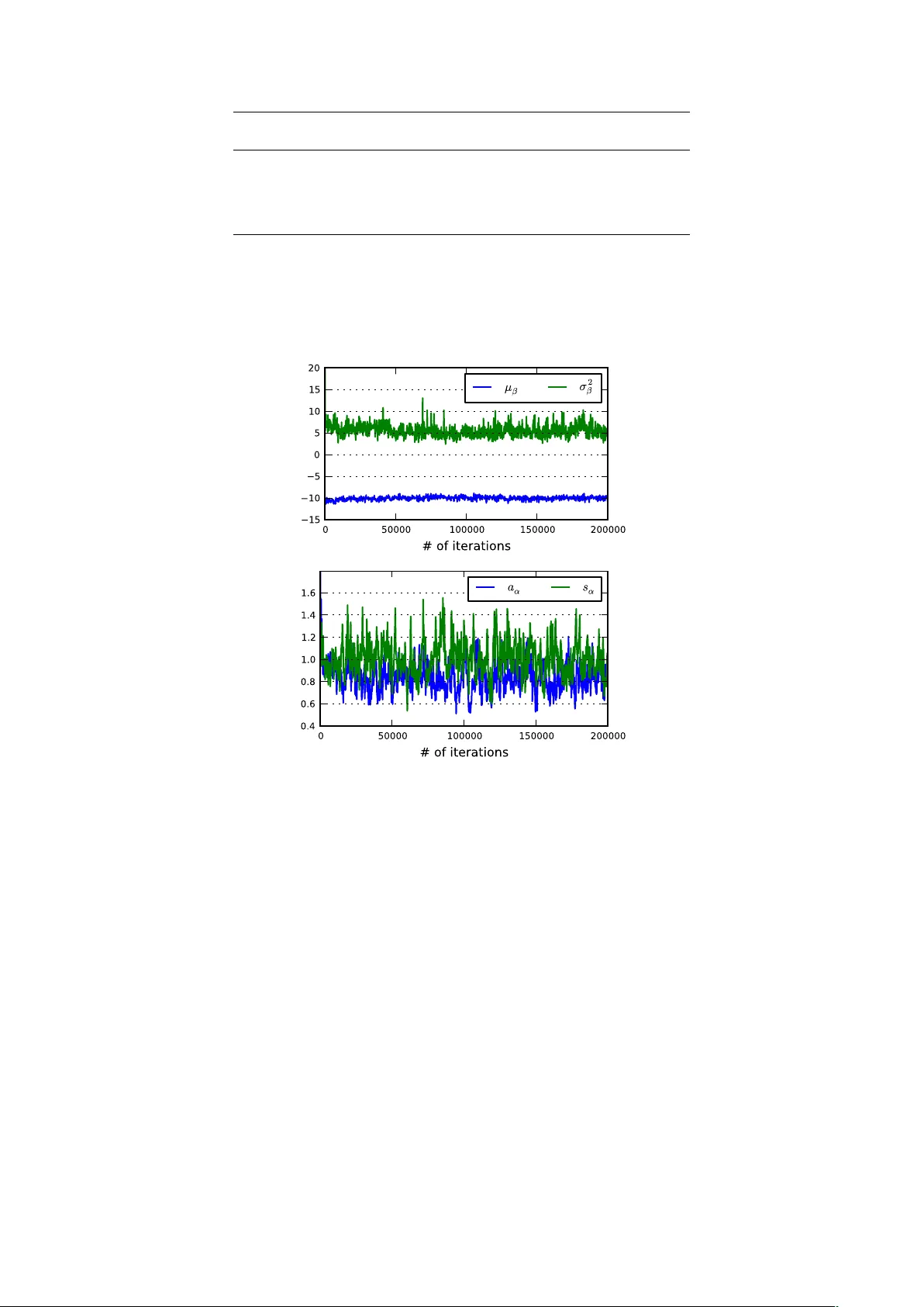
Non-parametric Ba y esian mo delling of digital gene expression data Dimitrios V. V a voulis 1 , ∗ and Julian Gough 1 , ∗ 1 Departmen t of Computer Science, Universit y of Bristol, Bristol, United Kingdom Jan uary 7, 2013 Abstract Next-generation sequencing technologies pro vide a revolutionary to ol for generating gene expres- sion data. Starting with a fixed RNA sample, they construct a library of millions of differentially abundan t short sequence tags or “reads”, which constitute a fundamen tally discrete measure of the lev el of gene expression. A common limitation in exp erimen ts using these technologies is the low n umber or even absence of biological replicates, which complicates the statistical analysis of digital gene expression data. Analysis of this type of data has often b een based on mo dified tests originally devised for analysing microarrays; b oth these and even de novo metho ds for the analysis of RNA-seq data are plagued by the common problem of low replication. W e propose a nov el, non-parametric Ba yesian approac h for the analysis of digital gene expression data. W e b egin with a hierarchical model for mo delling ov er-disp ersed count data and a blo c ked Gibbs sampling algorithm for inferring the posterior distribution of mo del parameters conditional on these counts. The algorithm comp ensates for the problem of lo w num b ers of biological replicates b y clustering together genes with tag counts that are likely sampled from a common distribution and using this augmen ted sample for estimating the parameters of this distribution. The num b er of clusters is not decided a priori , but it is inferred along with the remaining mo del parameters. W e demonstrate the abilit y of this approac h to mo del biological data with high fidelity by applying the algorithm on a public dataset obtained from cancerous and non-cancerous neural tissues. 1 1 In tro duction It is a common truth that our knowledge in Molecular Biology is only as go od as the to ols we ha ve at our disp osal. Next-generation or high-throughput sequencing technologies provide a revolutionary to ol in the aid of genomic studies by allowing the generation, in a relatively short time, of millions of short sequence tags, which reflect particular asp ects of the molecular state of a biological system. A common application of these technologies is the study of the transcriptome, which in volv es a family of metho dologies, including RNA-seq ([25]), CAGE (Cap Analysis of Gene Expression; [19]) and SA GE (Serial Analysis of Gene Expression; [22]). When compared to microarrays, this class of methodologies offers several adv antages, including detection of a wider level of expression levels and indep endence on prior knowledge of the biological system, which is required by h ybridisation-based technologies, such as microarra ys. T ypically , an exp erimen t in this category starts with the extraction of a snapshot RNA sample from the biological system of interest and its shearing in a large num b er of fragmen ts of v arying lengths. The p opulation of these fragments is then reversed-transcribed to a cDNA library and sequenced on a high- throughput platform, generating large num bers of short DNA sequences known as “reads”. The ensuing analysis pip eline starts with mapping or aligning these reads on a reference genome. At the next stage, the mapp ed reads are summarised into gene-, exon- or transcript-level counts, normalised and further analysed for detecting differential gene expression (see [15] for a review). It is imp ortan t to realize that the normalised read (or tag) count data generated from this family of metho dologies represen ts the num b er of times a particular class of cDNA fragments has b een sequenced, whic h is directly related to their abundance in the library and, in turn, the abundance of the asso ciated transcripts in the original sample. Thus, this count data is essentially a discrete or digital measure of ∗ to whom correspondence should be addressed 1 Python code is av ailable upon request. A user-friendly pac k age is currently under developmen t. 1 gene expression, which is fundamentally differen t in nature (and, in general terms, sup erior in quality) from the contin uous fluorescence intensit y measurements obtained from the application of microarra y tec hnologies. Due to their b etter quality , next-generation sequence assays tend to replace microarra y- based technologies, despite their higher cost ([4]). One approac h for the analysis of coun t data of gene expression is to transform the counts to approx- imate normality and then apply existing metho ds aimed at the analysis of microarra ys (see for example, [21, 5]). How ev er, as noted in [13], this approach may fail in the case of v ery small counts (which are far from normally distributed) and also due to the strong mean-v ariance relationship of count data, which is not tak en into account b y tests based on a normality assumption. Prop er statistical mo delling and analysis of count data of gene expression requires nov el approac hes, rather than adaptation of existing metho dologies, whic h aimed from the beginning at pro cessing contin uous input. F ormally , the generation of count data using next-generation sequencing assays can b e thought of as random sampling of an underlying p opulation of cDNA fragments. Thus, the counts for each tag describing a class of cDNA fragments can, in principle, b e mo delled using the P oisson distribution, whose v ariance is, b y definition, equal to its mean. Ho wev er, it has b een shown that, in real count data of gene expression, the v ariance can b e larger that what is predicted by the Poisson distribution ([12, 17, 18, 14]). An approac h that accounts for the so-called “o ver-dispersion” in the data is to adopt quasi-lik eliho o d metho ds, whic h augmen t the v ariance of the Poisson distribution with a scaling factor, th us b y-passing the assumption of equalit y betw een the mean and v ariance ([2, 20, 24, 11]). An alternative approac h is to use the Negative Binomial distribution, which is derived from the Poisson, assuming a Gamma-distributed rate parameter. The Negativ e Binomial distribution incorporates both a mean and a v ariance parameter, th us modelling ov er-dispersion in a natural wa y ([1, 7, 13]). An o verview of existing metho ds for the analysis of gene expression count data can b e found in [15] and [10] Despite the decreasing cost of next-generation sequencing assa ys (and also due to tec hnical and ethical restrictions), digital datasets of gene expression are often characterised b y a small num b er of biological replicates or no replicates at all. Although this complicates an y effort to statistically analyse the data, it has led to inv en tive attempts at estimating as accurately as p ossible the biological v ariabilit y in the data given very small samples. One approach is to assume a lo cally linear relationship b et ween the v ariance and the mean in the Negative Binomial distribution, whic h allo ws estimating the v ariance b y p ooling together data from genes with similar expression levels ([1]). Alternativ ely , one can make the rather restrictive assumption that all genes share the same v ariance, in which case the ov er-disp ersion parameter in the Negativ e Binomial distribution can b e estimated from a very large set of datap oin ts ([17]). A further elab oration of this approach is to assume a unique v ariance p er gene and adopt a w eighted-lik eliho od metho dology for sharing information b etw een genes, which allows for an improv ed estimation of the gene-sp ecific ov er-dispersion parameters ([13]). Another yet distinct empirical Bay es approac h is implemen ted in the soft ware b aySe q , whic h adopts a form of information sharing betw een genes by assuming the same prior distribution among the parameters of samples demonstrating a large degree of similarity ([7]). In summary , prop er statistical modelling and analysis of digital gene expression data requires the dev elopment of nov el metho ds, which take into account b oth the discrete nature of this data and the t ypically small num b er (or even the absence) of biological replicates. The developmen t of suc h metho ds is particularly urgent due to the huge amoun t of data b eing generated by high-throughput sequencing assa ys. In this paper, we presen t a method for modelling digital gene expression data that utilizes a no vel form of information sharing betw een genes (based on non-parametric Bay esian clustering) to compensate for the all-to o-common problem of low or no replication, which plagues most curren t analysis methods. 2 Approac h W e propose a nov el, non-parametric Bay esian approac h for the analysis of digital gene expression data. Our p oin t of departure is a hierarchical mo del for o ver-dispersed counts. The mo del is built around the Negativ e Binomial distribution, whic h dep ends, in our formulation, on tw o parameters: the mean and an ov er-disp ersion parameter. W e assume that these parameters are sampled from a Dirichlet pro cess with a join t Inv erse Gamma - Normal base distribution, which w e hav e implemen ted using stick breaking priors. By construction, the mo del imp oses a clustering effect on the data, where all genes in the same cluster are statistically describ ed by a unique Negative Binomial distribution. This can b e thought of as a form of information sharing betw een genes, whic h permits po oling together data from genes in the same cluster for improv ed estimation of the mean and ov er-disp ersion parameters, thus bypassing the problem of little or no replication. W e develop a blo c k ed Gibbs sampling algorithm for estimating the p osterior 2 ... ... ... ... ⋮ ⋮ ⋮ ⋮ ⋮ ⋮ ⋮ ⋮ ... ... ⋮ ⋮ ⋮ ⋮ ⋮ ⋮ ⋮ ⋮ ... ... ... ... classes samples exposure genes 1 l L j +1 1 j 2 M  1 M y NM  1 y NM y i 1 y i 2 y N 1 y N 2 y Nj y Nj +1 y ij +1 y ij y iM  1 y iM c 1 c 2 c j c j +1 c M  1 c M p ( Y il | ↵ il ,  il )= Y j NegBinomial( y ij | ↵ i  ( j ) ,c j e  i  ( j ) ) Figure 1: F ormat of digital gene expression data. Rows corresp ond to genes and columns corresp ond to samples. Samples are grouped in to classes (e.g. tissues or exp erimental conditions). Eac h element of the data matrix is a whole n umber indicating the num ber of counts or reads corresponding to the i th gene at the j th sample. The sum of the reads across all genes in a sample is the depth or exp osure of that sample. distributions of the v arious free parameters in the model. These include the mean and o ver-dispersion for eac h gene and the n umber of clusters (and their o ccupancies), whic h do es not need to b e fixed a priori , as in alternative (parametric) clustering metho ds. In principle, the prop osed method can b e applied on v arious forms of digital gene expression data (including RNA-seq, CA GE, SAGE, T ag-seq, etc.) with little or no replication and it is actually applied on one suc h example dataset herein. 3 Mo delling o v er-disp ersed coun t data The digital gene expression data we are considering is arranged in an M × N matrix, where each of the N ro ws corresp onds to a different gene and each of the M columns corresp onds to a different sample. F urthermore, all samples are group ed in L different classes (i.e. tissues or exp erimental conditions). It holds that L ≤ M , where the equality is true if there are no replicas in the data. W e indicate the n umber of reads for the i th gene at the j th sample with the v ariable y ij . W e assume that y ij is Poisson-distributed with a gene- and sample-sp ecific rate parameter r ij . The rate parameter r ij is assumed random itself and it is mo delled using a Gamma distribution with shap e parameter α iλ ( j ) and scale parameter s ij . The function λ ( · ) in the subscript of the shap e parameter maps the sample index j to an integer indicating the class this sample b elongs to. Th us, for a particular gene and class, the shap e of the Gamma distribution is the same for all samples. Under this setup, the rate r ij can b e in tegrated (or marginalised) out, whic h giv es rise to the Negative Binomial distribution with parameters α iλ ( j ) and µ ij = α iλ ( j ) s ij for the num b er of reads y ij : y ij | α iλ ( j ) , µ ij ∼ Γ( y ij + α iλ ( j ) ) Γ( α iλ ( j ) )Γ( y ij + 1)  α iλ ( j ) α iλ ( j ) + µ ij  α iλ ( j )  µ iλ ( j ) α iλ ( j ) + µ ij  y ij (1) where µ ij is the mean of the Negative Binomial distribution and µ ij + α − 1 iλ ( j ) µ 2 ij is the v ariance. Since the v ariance is alwa ys larger than the mean b y the quan tity α − 1 iλ ( j ) µ 2 ij , the Negativ e Binomial distribution can b e thought of as a generalisation of the P oisson distribution, which accounts for o ver-dispersion. F urthermore, we mo del the mean as µ ij = c j e β iλ ( j ) , where the offset c j = P N i =1 y ij is the depth or exp o- sure of sample j and β iλ ( j ) is, similarly to α iλ ( j ) , a gene- and class-specific parameter. This formulation ensures that µ ij is alwa ys positive, as it oughts to. Giv en the mo del ab ov e, the likelihoo d of observed reads Y il = { y ij : λ ( j ) = l } for the i th gene in class 3 l is written as follows: p ( Y il | α il , β il ) = Y j p ( y ij | α iλ ( j ) , β iλ ( j ) ) = Y j NegBinomial( y ij | α iλ ( j ) , c j e β iλ ( j ) ) (2) where the index j satisfies the condition λ ( j ) = l . By extension, for the i th gene across all sample classes, the likelihoo d of observ ed counts Y i = { y ij : λ ( j ) = l , l = 1 , . . . , L } is written as: p ( Y i | α i 1 , β i 1 , . . . , α iL , β iL ) = Y l p ( Y il | α il , β il ) (3) where the class indicator l runs across all L classes. 3.1 Information sharing b etw een genes A common feature of digital gene expression data is the small n umber of biological replicates p er class, whic h mak es any attempt to estimate the gene- and class-sp ecific parameters θ il = { α il , β il } through standard likelihoo d metho ds a futile exercise. In order to make robust estimation of these parameters feasible, some form of information sharing b et ween different genes is necessary . In the present context, information sharing b et ween genes means that not all v alues of θ il are distinct; differen t genes (or the same gene across differen t sample classes) may share the same v alues for these parameters. This idea can b e expressed formally by assuming that θ il is random with an infinite mixture of discrete random measures as its prior distribution: θ il ∼ ∞ X k =1 w k δ θ ∗ k , 0 ≤ w k ≤ 1 , ∞ X k =1 w k = 1 (4) where δ θ ∗ k indicates a discrete random measure centered at θ ∗ k = { α ∗ k , β ∗ k } and w k is the corresp onding w eight. Conceptually , the fact that the ab o ve summation go es to infinity expresses our lack of prior kno wledge regarding the num b er of comp onen ts that app ear in the mixture, other than the obvious restriction that their maximum n umber cannot be larger than the n umber of genes times the num b er of sample classes. In this formulation, the parameters θ ∗ k are sampled from a prior base distribution G 0 with hyper- parameters φ , i.e. θ ∗ k | φ ∼ G 0 ( φ ). W e assume that α ∗ k is distributed according to an inv erse Gamma distribution with shap e a α and scale s α , while β ∗ k follo ws the Normal distribution with mean µ β and v ariance σ 2 β . Thus, G 0 is a joint distribution as follo ws: θ ∗ k z }| { α ∗ k , β ∗ k | φ z }| { a α , s α , µ β , σ 2 β ∼ G 0 ( φ ) z }| { In vGamma( a α , s α ) · Normal( µ β , σ 2 β ) , k = 1 , 2 , . . . (5) Giv en the abov e, α ∗ k can take only p ositiv e v alues, as it oughts to, while β ∗ k can take b oth p ositive and negativ e v alues. What makes the mixture in Eq. 4 sp ecial is the pro cedure for generating the infinite sequence of mixing weigh ts. W e set w 1 = V 1 and w k = V k Q k − 1 m =1 (1 − V m ) for k ≥ 2, where { V 1 , . . . , V k } are random v ariables following the Beta distribution, i.e. V k ∼ Beta( a k , b k ). This constructiv e wa y of sampling new mixing w eights resem bles a stic k-breaking process; generating the first w eight w 1 corresp onds to breaking a stic k of length 1 at p osition V 1 ; generating the second weigh t w 2 corresp onds to breaking the remaining piece at p osition V 2 and so on. Thus, we write: w k | a k , b k ∼ Stick( a k , b k ) , k = 1 , 2 , . . . (6) There are v arious wa ys for defining the parameters a k and b k . Here, we consider only the case where a k = 1 and b k = η , with η > 0. This parametrisation is equiv alent to setting the prior of θ il to a Diric hlet Pro cess with base distribution G 0 and concentration parameter η . By construction, this procedure leads to a rapidly decreasing sequence of sampled weigh ts, at a rate whic h dep ends on η . F or v alues of η m uch smaller than 1, the w eights w k decrease rapidly with increasing k , only one or few w eights ha ve significan t mass and the parameters θ il share a single or a small n umber of different v alues θ ∗ k . F or v alues of the 4 Clas s 1 Cla ss 1 Clas s 2 Cla ss 2 Sample 1 Sample 2 Sample 3 Sample 4 ⋮ Class 1 Class 2 Cluster weights Cluster indicators Data ⌘ w 1 w 2 w 3 w 4 w 5 z 11 z 12 z 21 z 22 z 31 z 32 z 41 z 42 z 51 z 52 z 61 z 62 y 11 y 12 y 13 y 14 y 21 y 22 y 23 y 24 y 31 y 32 y 33 y 34 y 41 y 42 y 43 y 44 y 51 y 52 y 53 y 54 y 61 y 62 y 63 y 64 Figure 2: The clustering effect that results from imp osing a stick-breaking prior on the gene- and class- sp ecific mo del parameters, θ il . A matrix of indicator v ariables is used to cluster the observed count data in to a finite num b er of groups, where the genes in eac h group share the same mo del parameters. The n umber of clusters is not known a priori . The distribution of w eight mass among the v arious clusters in the mo del is determined by parameter η . concen tration parameter muc h larger than 1, the w eights w k decrease slowly with increasing k , many w eights hav e significan t mass and the v alues of θ il tend to b e all distinct to eac h other and distributed according to G 0 . Below, we set η = 1, whic h results in a balanced decrease of the weigh t mass with increasing k . In particular, for η = 1, log ( w k ) decreases (on av erage) in an un biased manner with increasing k . Giv en the ab o ve formulation, sampling θ il from its prior distribution is straigh tforward. First, w e in tro duce an indicator v ariable z il ∈ { 1 , 2 , . . . } , which points to the v alue of θ ∗ k corresp onding to the i th gene in class l . W e sample such indicator v ariables for eac h gene in each class from the Categorical distribution, i.e. z il ∼ Categorical( w 1 , w 2 , . . . ), and set θ il ≡ θ ∗ z il . Although G 0 is contin uous, the distribution of θ il is almost surely discrete and, therefore, its v alues are not all distinct. Different genes ma y share the same v alue of θ ∗ and, thus, all genes are group ed in a finite (unkno wn) num b er of clusters, according to the v alue of θ ∗ k they share. Modelling digital gene expression data using this approac h is one w ay to bypass the problem of few (or the absence of ) technical replicates, since the data from all genes in the same cluster are p o oled together for estimating the parameters that c haracterise this cluster. The clustering effect describ ed in this section is illustrated in Fig. 2. 3.2 Generativ e mo del The description in the previous paragraphs suggests a hierarchical mo del, which presumably underlies the sto c hastic generation of the data matrix in Fig. 1. This model is explicitly describ ed below: θ ∗ k | a α , s α , µ β , σ 2 β ∼ In vGamma( a α , s α ) · Normal( µ β , σ 2 β ) w 1 , w 2 , . . . | η ∼ Stic k(1 , η ) z iλ ( j ) | w 1 , w 2 , . . . ∼ Categorical( w 1 , w 2 , . . . ) θ iλ ( j ) ≡ θ ∗ z iλ ( j ) y ij | θ iλ ( j ) ∼ NegBinomial  θ iλ ( j )  (7) A t the b ottom of the hierarc hy , we iden tify the measured reads y ij for each gene in each sample, which follo w a Negative Binomial distribution with parameters θ iλ ( j ) = { α iλ ( j ) , β iλ ( j ) } . The parameters of the Negativ e Binomial distribution θ iλ ( j ) are gene- and class-sp ecific and they are completely determined b y an also gene- and class-specific indicator v ariable z iλ ( j ) and the cen ters θ ∗ k of the infinite mixture of p oin t measures in Eq. 4. These cen ters are distributed according to a joint inv erse Gamma and Normal distribution with hyper-parameters φ = { a α , s α , µ β , σ 2 β } , while the indicator v ariables are sampled from a Categorical distribution with weigh ts { w 1 , w 2 , . . . } . These are, in turn, sampled from a stick-breaking pro cess with concentration parameter η . In this mo del, φ , w k , θ ∗ k and z iλ ( j ) are laten t v ariables, which are sub ject to estimation based on the observed data. 5 4 Inference A t this point, we introduce some further notation. W e indicate the N × L matrix of indicator v ariables with the letter Z ; Θ ∗ = { θ ∗ 1 , θ ∗ 2 , . . . } lists the cen ters of the point measures in Eq. 4 and W = { w 1 , w 2 , . . . } is the vector of mixing w eights. W e are interested in computing the joint p osterior densit y p ( Z , W , Θ ∗ , φ | Y ), where Y is a matrix of count data as in Fig. 1. W e approximate the abov e distribution through numerical (Mon te Carlo) metho ds, i.e. by sampling a large n umber of { Θ ∗ , W, Z , φ } -tuples from it. One wa y to achiev e this is by constructing a Mark ov chain, whic h admits p ( Z, W, Θ ∗ , φ | Y ) as its stationary distribution. Suc h a Marko v c hain can b e constructed by using Gibbs sampling, which consists of alternating rep eated sampling from the full conditional posteriors p (Θ ∗ | Y , Z , φ ), p ( W | Z ), p ( Z | Y , Θ ∗ , W ) and p ( φ | Θ ∗ , Z ). Belo w, we explain ho w to sample from each of these conditional distributions. Sampling from the conditional p osterior p (Θ ∗ | Y , Z , φ ) In order to sample from the abov e distribution it is con venien t to truncate the infinite mixture in Eq. 4 b y rejecting all terms with index larger than K and setting w K = 1 − P K − 1 k =1 w k , whic h is equiv alent to setting V K = 1. It has b een shown that the error asso ciated with this approximation when V k ∼ Beta(1 , η ) is less than or equal to 4 N M exp( − K − 1 η ) ([8]). F or example, for N = 14 × 10 3 , M = 6, K = 200 and η = 1, the error is minimal (less than 10 − 80 ). Thus, the truncation should b e virtually indistinguishable from the full (infinite) mixture. Next, w e distinguish b et ween K ac activ e clusters (Θ ∗ ac ) and K in inactiv e clusters (Θ ∗ in ), suc h that Θ ∗ = { Θ ∗ ac , Θ ∗ in } and K = K ac + K in . Active clusters are those containing at least one gene, while those con taining no genes are considered inactive. W e write: p (Θ ∗ | Y , Z , φ ) = p (Θ ∗ ac , Θ ∗ in | Y , Z , φ ) = p (Θ ∗ ac | Y , Z , φ ) p (Θ ∗ in | φ ) Up dating the inactiv e clusters is a simple matter of sampling K in times from the join t distribution in Eq. 5 given the hyper-parameters φ . Sampling the activ e clusters is more complicated and inv olves sampling eac h activ e cluster center θ ∗ ac,k individually from its resp ectiv e posterior, p ( θ ∗ ac,k | Y ac,k ), where Y ac,k is a matrix of measured coun t data for all genes in the k th activ e cluster. Sampling θ ∗ ac,k = { α ∗ ac,k , β ∗ ac,k } is done using the Metrop olis algorithm with acceptance probability: P acc = min 1 , p ( Y ac,k | θ + ac,k ) p ( Y ac,k | θ ∗ ac,k ) p ( θ + ac,k | φ ) p ( θ ∗ ac,k | φ ) ! (8) where the sup erscript + indicates a candidate vector of parameters. Each of the tw o elemen ts ( α and β ) of this vector is dra wn from a symmetric prop osal of the follo wing form: q ( x + | x ∗ ) = x ∗ exp(0 . 01 · r ) (9) where the random num b er r is sampled from the standard Normal distribution, i.e. r ∼ Normal(0 , 1). The prior of p ( θ ∗ ac,k | φ ) is a join t Inv erse Gamma - Normal distribution, as shown in Eq. 5, while the lik eliho o d function p ( Y ac,k | θ ∗ ac,k ) is a pro duct of Negativ e Binomial probabilit y distributions, similar to those in Eqs. 2 and 3. Sampling from the conditional p osterior p ( Z | Y , Θ ∗ , W ) Eac h element z il of the matrix of indicator v ariables Z is sampled from a Categorical distribution with w eights π il = { π 1 il , . . . , π K il } , where π k il = Π k il / P K m =1 Π m il and: { Π 1 il , . . . , Π K il } ∝ { w 1 p ( Y il | θ ∗ 1 ) , . . . , w K p ( Y il | θ ∗ K ) } (10) In the ab o ve expression, Y il is the data for the i th gene in class l , as mentioned in a previous section. Notice that z il can take any integer v alue b et ween 1 and K and that the weigh ts π il dep end b oth on the cluster weigh ts w k and on the v alue of the likelihoo d function p ( Y il | θ ∗ k ). 6 Sampling from the conditional p osterior p ( W | Z ) The mixing w eights W are generated using a truncated stic k-breaking pro cess with η = 1. As pointed out in [8], this implies that W follows a generalised Diric hlet distribution. Considering the conjugacy b etw een this and the m ultinomial distribution, the first step in updating W is to generate K − 1 Beta-distributed random num b ers: V k ∼ Beta(1 + N k , η + N − k X m =1 N m ) (11) for k = 1 , . . . , K − 1, where N k is the total num b er of genes in the k th cluster. Notice that N k can b e inferred from Z b y simple counting and P K m =1 N k = N , where N is the total num b er of genes. V K is set equal to 1, in order to ensure that the w eights add up to 1. These are simply generated by setting V 1 = w 1 and w k = V k Q k − 1 m =1 (1 − V m ), as mentioned in a previous section. Sampling from the conditional p osterior p ( φ | Θ ∗ , Z ) The hyper-parameters φ = { a α , s α , µ β , σ 2 β } influence indirectly the observ ations Y through their effect on the distribution of the active cluster centers, Θ ∗ ac = { α ∗ ac , β ∗ ac } , where α ∗ ac = { α ∗ ac, 1 , . . . , α ∗ ac,K ac } and β ∗ ac = { β ∗ ac, 1 , . . . , β ∗ ac,K ac } . If we further assume indep endence b et ween α ∗ ac and β ∗ ac , w e can write p ( φ | Θ ∗ , Z ) = p ( a α , s α , µ β , σ 2 β | α ∗ ac , β ∗ ac ) = p ( a α , s α | α ∗ ac ) p ( µ β , σ 2 β | β ∗ ac ). Assuming K ac activ e clusters and considering that the prior for α ∗ is an In verse Gamma distribution (see Eq. 5), it follo ws that the p osterior p ( a α , s α | α ∗ ac ) is: p ( a α , s α | α ∗ ac ) ∝ γ a α − 1 1 exp( − s α γ 2 ) s a α γ 3 α Γ( a α ) γ 4 (12) The parameters γ 1 to γ 4 are given by the following expressions: γ 1 = γ (0) 1 K ac Y k =1 1 α ∗ ac,k γ 2 = γ (0) 2 + K ac X k =1 1 α ∗ ac,k γ 3 = γ (0) 3 + K ac γ 4 = γ (0) 4 + K ac where the initial parameters γ (0) 1 , γ (0) 2 , γ (0) 3 and γ (0) 4 are all p ositiv e. Since sampling from Eq. 12 cannot b e done exactly , we emplo y a Metrop olis algorithm with acceptance probabilit y P acc = min  1 , p ( a + α , s + α | α ∗ ac ) p ( a α , s α | α ∗ ac )  (13) where the prop osal distribution q ( ·|· ) for sampling new candidate p oin ts has the same form as in Eq. 9. F urthermore, taking adv antage of the conjugacy betw een a Normal likelihoo d and a Normal-In verseGamma prior, the p osterior probabilit y for parameters µ β and σ 2 β b ecomes: p ( µ β , σ 2 β | β ∗ ac ) = NormalIn verseGamma( δ 1 , δ 2 , δ 3 , δ 4 ) (14) The parameters δ 1 to δ 4 (giv en initial parameters δ (0) 1 to δ (0) 4 ) are as follows: δ 1 = δ (0) 1 δ (0) 2 + K ac ¯ β ∗ ac δ (0) 2 + K ac δ 2 = δ (0) 2 + K ac δ 3 = δ (0) 3 + K ac 2 δ 4 = δ (0) 4 + 1 2 K ac X k =1 ( β ∗ ac,k − ¯ β ∗ ac ) + 1 2 δ (0) 2 K ac δ (0) 2 + K ac ( ¯ β ∗ ac − δ (0) 1 ) 7 where ¯ β ∗ ac = 1 K ac P K ac k =1 β ∗ ac,k . Sampling a { µ β , σ 2 β } -pair from the abov e posterior tak es place in t wo simple steps: first, we sample σ 2 β ∼ Inv erseGamma( δ 3 , δ 4 ), where δ 3 and δ 4 are shap e and scale parameters, resp ectiv ely . Then, we sample µ β ∼ Normal( δ 1 , σ 2 β /δ 2 ). 4.1 Algorithm W e summarise the algorithm for drawing samples from the posterior p (Θ ∗ , Z, W , φ | Y ) below. Notice that x ( t ) indicates the v alue of x at the t th iteration of the algorithm. x (0) is the initial v alue of x . 1. Set γ (0) = n γ (0) 1 , γ (0) 2 , γ (0) 3 , γ (0) 4 o 2. Set δ (0) = n δ (0) 1 , δ (0) 2 , δ (0) 3 , δ (0) 4 o 3. Set φ (0) = { a (0) α , b (0) α , µ (0) β , σ 2(0) β } 4. Set K , the truncation level 5. Sample Θ ∗ (0) from its prior (Eq. 5) conditional on φ (0) 6. Set all K elemen ts of W (0) to the same v alue, i.e. 1 /K 7. Sample Z (0) from the Categorical distribution with w eights W (0) 8. F or t = 1 , 2 , 3 , . . . , T (a) Sample Θ ∗ ( t ) ac giv en Z ( t − 1) , φ ( t − 1) and the data matrix Y using a single step of the Metropolis algorithm for each activ e cluster (see Eq. 8) (b) Sample Θ ∗ ( t ) in from its prior given φ ( t − 1) (see Eq. 5) (c) Sample Z ( t ) giv en Θ ∗ ( t ) , W ( t − 1) and the data matrix Y (see Eq. 10) (d) Sample W ( t ) giv en Z ( t ) (see Eq. 11) (e) Sample φ ( t ) giv en Θ ∗ ( t ) ac and φ ( t − 1) (see Eqs. 12 and 14) 9. Discard the first T 0 samples, which are pro duced during the burn-in p erio d of the algorithm (i.e. b efore equilibrium is attained), and work with the remaining T − T 0 samples. The ab ov e pro cedure implements a form of blo c ked Gibbs sampling with em b edded Metrop olis steps for imp ossible to directly sample from distributions. 5 Results and Discussion W e hav e implemented the metho dology describ ed in the preceding sections in softw are and we hav e applied this soft ware on publicly a v ailable digital gene expression data (obtained from control and can- cerous tissue cultures of neural stem cells; [6]) for ev aluation purp oses. The data we used in this study can b e found at the following URL: http://genomebiology .com/con tent/supplemen tary/gb-2010-11-10- r106-s3.tgz. As sho wn in T able 1, this dataset consists of four libraries from glioblastoma-deriv ed neural stem cells and t wo from non-cancerous neural stem cells. Each tissue culture w as deriv ed from a different sub ject. Thus, the samples are divided in tw o classes (cancerous and non-cancerous) with four and tw o replicates, resp ectiv ely . W e implemented the algorithm presented ab ov e in the programming language Python, using the libraries NumPy , SciPy and MatplotLib. Calculations w ere expressed as operations betw een arrays and the multipr o c essing Python module w as utilised in order to tak e full adv antage of the parallel arc hitecture of modern multicore pro cessors. The algorithm was run for 200K iterations, which to ok approximately t wo days to complete on a 12-core desktop computer. Simulation results were sav ed to the disk every 50 iterations. The raw simulation output includes chains of random v alues of the hyper-parameters φ , the gene- and class-sp ecific indicators Z and the active cluster centers Θ ∗ ac , which constitute an approximation to the corresp onding p osterior distributions given the data matrix Y . The c hains corresp onding to the four differen t comp onen ts of φ = { a α , s α , µ β , σ 2 β } are illustrated in Figure 3. It may be observ ed that these 8 Cancerous Non-cancerous Genes GliNS1 G144 G166 G179 CB541 CB660 13CDNA73 4 0 6 1 0 5 15E1.2 75 74 222 458 215 167 182-FIP 118 127 555 231 334 114 . . . . . . . . . . . . . . . . . . . . . T able 1: F ormat of the data b y [6]. The first four samples are from glioblastoma neural stem cells, while the last t wo are from non-cancerous neural stem cells. The dataset contains a total of 18760 genes (i.e. ro ws). A B Figure 3: Sim ulation results after 200K iterations. The chains of random samples corresp ond to the comp onen ts of the v ector of h yp er-parameters φ , i.e. µ β and σ 2 β (panel A) and a α and s α (panel B). The former determines the Normal prior distribution of the cluster center parameters β ∗ , while the latter pair determines the In verse Gamma prior distribution of the cluster center parameters α ∗ . The random samples in each c hain are appro ximately sampled (and constitute an approximation of ) the corresp onding p osterior distribution conditional on the data matrix Y . reac hed equilibrium early during the sim ulation (after less than 20K iterations) and they remained stable for the remaining of the simulation. As explained earlier, these hyper-parameters are imp ortant, because they determine the prior distributions of the cluster centers α ∗ and β ∗ (h yp er-parameters { a α , s α } and { µ β , σ 2 β } , resp ectiv ely) and, subsequently , of the gene- and class-specific parameters α and β . It follows from analysis of the chains in Figure 3 that the estimates for these hyper-parameters are (indicating the mean and standard deviation of the estimates): a α = 0 . 83 ± 0 . 13, s α = 1 . 00 ± 0 . 16, µ β = − 10 . 01 ± 0 . 39 and σ 2 β = 5 . 41 ± 1 . 32. The corresp onding Inv erse Gamma and Normal distributions, whic h are the priors of the cluster centers α ∗ and β ∗ , resp ectiv ely , are illustrated in Figure 4. A ma jor use of the methodology presen ted ab o ve is that it allo ws us to estimate the gene- and class-sp ecific parameters α and β , under the assumption that the same v alues for these parameters are shared b et ween differen t genes or even b y the same gene among different sample classes. This form of information sharing p ermits pulling together data from different genes and classes for estimating pairs of α and β parameters in a robust wa y , ev en when only a small n umber of replicates (or no replicates at all) are a v ailable p er sample class. As an example, in Figure 5 we illustrate the c hains of random samples 9 A B Figure 4: Estimated Inv erse Gamma (panel A) and Normal (panel B) prior distributions for the cluster parameters α ∗ and β ∗ , resp ectiv ely . The solid lines indicate mean distributions, i.e. those obtained for the mean v alues of the hyper-parameters a α , s α , µ β and σ 2 β . The dashed lines are distributions obtained b y adding or subtracting individually one standard deviation from eac h relev ant h yp er-parameter. for α and β corresp onding to the non-cancerous class of samples for the tag with ID 182-FIP (third ro w in T able 1). These samples constitute approximations of the p osterior distributions of the corresp onding parameters. Despite the very small n umber of replicates ( n = 4), the v ariance of the random samples is finite. Similar chains were derived for each gene in the dataset, although it should be emphasised that the num b er of suc h estimates is smaller than the total num b er of genes, since more than one genes share the same parameter estimates. It has already been mentioned that the sharing of α and β parameter v alues b et ween different genes can b e viewed as a form of clustering (see Figure 2), i.e. there are different groups of genes, where all genes in a particular group share the same α and β parameter v alues. As exp ected in a Ba yesian inference framework, the n umber of clusters is not constant, but it is itself a random v ariable, which is c haracterised by its o wn p osterior distribution and its v alue fluctuates randomly from one iteration to the next. In Figure 6, w e illustrate the chain of sampled cluster num b ers during the course of the sim ulation (panel A). The first 75K iterations were discarded as burn-in and the remaining samples w ere used for plotting the histogram in panel B, which appro ximates the p osterior distribution of the n umber of clusters given the data matrix Y . It ma y b e observ ed that the n umber of clusters fluctuates b et w een 35 and 55 with a peak at around 42 clusters. The algorithm w e presen t ab o v e do es not mak e an y particular assumptions regarding the n umber of clusters, apart from the obvious one that this num b er cannot exceed the n umber of genes times the num b er of sample libraries. Although the truncation level K = 200 sets an artificial limit in the maximum n umber of clusters, this is nev er a problem in practise, since the actual estimated num b er of clusters is t ypically muc h smaller that the truncation lev el K (see the y-axis in Figure 6A). The fact that the num b er of clusters is not decided a priori, but rather inferred along with the other free parameters in the mo del sets the describ ed methodology in an adv antageous p osition with resp ect to alternative clustering algorithms, whic h require deciding the num b er of clusters at the b eginning of the simulation ([9]). Similarly to the sto c hastic fluctuation in the n umber of clusters, the cluster o ccupancies (i.e. the n umber of genes p er cluster) is a random vector. In Figure 7, w e illustrate the cluster o ccupancies at t wo different stages of the simulation, i.e. after 100K and 200K iterations, resp ectiv ely . W e ma y observ e that, with the exception of a single super-cluster (con taining more than 6000 genes), cluster occupancies range from b et ween around 3000 and less than 1000 genes. 10 A B Figure 5: Chains of random samples appro ximating the p osterior distributions of the parameters α (panel A) and β (panel B) corresponding to the non-cancerous class of samples for the tag with ID 182-FIP (third row in T able 1). These samples w ere generated after 200K iterations of the algorithm. A similar pair of chains exists for each gene at eac h sample class (i.e. cancerous and non-cancerous), although not all pairs are distinct to eac h other due to the clustering effect imp osed on the data by the algorithm. It should b e clarified that each cluster includes many (p oten tially , hundreds of ) genes and it may span sev eral classes. An individual cluster represents a Negative Binomial distribution (with concrete α and β parameters), whic h mo dels with high probability the coun t data from all its mem b er genes. This is illustrated in Figure 8, where we show the histogram of the log of the count data from the first sample (sample GliNS1 in T able 1) along with a subset of the estimated clusters after 200K iterations (gray lines) and the fitted mo del (red line). It may b e observ ed that eac h cluster mo dels a subset of the gene expression data in the particular sample. The complete model describing the whole sample is a w eighted sum of the individual clusters/Negative Binomial distributions. F ormally , p ( Y j | α 1 λ ( j ) , β 1 λ ( j ) , . . . , α N λ ( j ) , β N λ ( j ) ) = 1 N N X i =1 p ( y ij | α iλ ( j ) , β iλ ( j ) ) (15) where Y j is the j th sample and the index i runs o ver all N genes. W e rep eat that not all { α iλ ( j ) , β iλ ( j ) } pairs are distinct. Also, clusters with larger membership (i.e. including a larger num b er of genes) hav e larger weigh t in determining the ov erall model. The proposed metho dology pro vides a compact w ay to model each sample in a digital gene expression dataset following a tw o-step procedure: first, the dataset is partitioned into a finite num b er of clusters, where eac h cluster represen ts a Negativ e Binomial distribution (modelling a subset of the data) and the parameters of each suc h distribution are estimated. Subsequently , each sample in the dataset can b e mo delled as a weigh ted sum of Negative Binomial distributions. In Figure 9, we sho w the log of count data for each sample in the dataset sho wn in T able 1 along with the fitted mo dels (red lines) after 200K iterations of the algorithm. 6 Conclusion Next-generation sequencing technologies are routinely b eing used for generating huge volumes of gene expression data in a relativ ely short time. This data is fundamentally discrete in nature and their 11 A B Figure 6: Sto c hastic evolution of the num b er of clusters during 200K iterations of the sim ulation (panel A) and the resulting histogram after discarding the first 75K iterations as burn-in (panel B). After reac hing equilibrium, the n umber of clusters fluctuates around a mean of appro ximately 43 clusters. In general, the estimated num b er of clusters is m uch smaller than the truncation level ( K = 200, see y-axis in panel A). The histogram in panel B approximates the posterior distribution of the n umber of clusters giv en the data matrix Y . Figure 7: Cluster o ccupancies after 100K and 200K iterations of the algorithm. A single sup er-cluster (including more then 6000 genes) appears at both stages of the sim ulation. The occupancy of the remain- ing clusters demonstrates some v ariability during the course of the simulation, with clusters con taining b et w een 3000 and less than 1000 genes. 12 Figure 8: Histogram of the log of the num b er of reads from sample GliNS1, a subset of the estimated clusters (gray lines) and the estimated mo del of the sample at the end of the simulation. Each cluster (gra y line) represen ts a Negativ e Binomial distribution with sp ecific α and β parameters, which mo dels a subset of the coun t data in this particular sample. The complete mo del (red line) is the weigh ted sum of all comp onen t clusters. Ai Bi Aii Bii Aiii Aiv Gl1NS1 G144 G166 G179 CB541 CB660 Figure 9: Histograms of the log of the num b er of reads from cancerous (panels Ai-iv) and non-cancerous (panels Bi,ii) samples and the resp ectiv e estimated mo dels after 200K iterations of the algorithm. As already men tioned, eac h red line is the w eighted sum of man y component Negative Binomial distributions / clusters, whic h model different subsets of eac h data sample. W e ma y observ e that the estimated models fit tightly the corresponding data samples. 13 analysis requires the dev elopment of nov el statistical methods, rather than mo difying existing tests that w ere originally aimed at the analysis of microarra ys. The dev elopment of such metho ds is an active area of research and sev eral pap ers hav e been published on the sub ject (see [15] and [10] for an ov erview). In this pap er, we presen t a nov el approach for mo delling o ver-dispersed count data of gene expression (i.e. data with v ariance larger than the mean predicted by the P oisson distribution) using a hierarc hical mo del based on the Negative Binomial distribution. The nov el asp ect of our approach is the use of a Dirichlet pro cess in the form of stic k breaking priors for mo delling the parameters (mean and ov er- disp ersion) of the Negativ e Binomial distribution. By construction, this form ulation forces clustering of the count data, where genes in the same cluster are sampled from the same Negative Binomial distribution, with a common pair of mean and ov er-disp ersion parameters. Through this elegant form of information sharing b et ween genes, we comp ensate for the problem of little or no replication, which often restricts the analysis of digital gene expression datasets. W e hav e demonstrated the abilit y of this approac h to mo del accurately actual biological data b y applying the prop osed methodology on a publicly a v ailable dataset obtained from cancerous and non-cancerous cultured neural stem cells ([6]). W e show that inference is achiev ed in the prop osed mo del through the application of a blo ck ed Gibbs sampler, which includes estimating, among others, the gene- and class-specific mean and o ver-dispersion of the Negative Binomial distribution. Similarly , the num b er of clusters and their o ccupancies are inferred along with the rest free parameters in the mo del. Curren tly , the softw are implemen ting the prop osed metho d remains relativ ely computationally ex- p ensiv e. In particular, 200K iterations require approximately tw o da ys to complete on a 12-core desktop computer. This time scale is not disprop ortionate to the pro duction time of experimental data and it is mainly due to the high volume of the tested data ( > 15 K genes per sample) and the need to obtain long c hains of samples for a more accurate estimation of p osterior distributions. Long execution times are a c haracteristic, more generally , of all Monte Carlo approximation metho ds. Our implemen tation of the algorithm is completely parallelised and calculations are expressed as operations b et ween v ectors in order to take full adv an tage of mo dern multi-core computers. Ongoing w ork to wards reducing execution times aims at the application of v ariational inference metho ds ([3]), instead of the blo c ked Gibbs sampler w e curren tly use. The algorithm can b e further impro ved b y av oiding truncation of the infinite summation describ ed in Equation 4, as describ ed in [16] and in [23]. This non-parametric Ba yesian approach for mo delling count data has thus shown great promise in handling ov er-disp ersion and the all-to o-common problem of low replication, b oth in theoretical ev alu- ation and on the example dataset. The softw are that has b een produced will be of great utility for the study of digital gene expression data and the statistical theory will con tribute to leading the dev elopment of non-parametric metho ds in general for all forms of mo delling coun t data of gene expression. Ac kno wledgemen t The authors would like to thank Prof. P eter Green and Dr. Richard Goldstein for useful discussions. Also, w e would lik e to thank P . G. Engstrom and colleagues for pro ducing the public data w e used in this pap er. F unding: This work was supp orted b y grants EPSR C EP/H032436/1 and BBSR C G022771/1. References [1] Simon Anders and W olfgang Hub er. Differential expression analysis for sequence count data. Genome Biol , 11(10):R106, 2010. [2] P . L. Auer and R. W. Doerge. A Tw o-Stage P oisson Mo del for T esting RNA-Seq Data. Statistic al Applic ations in Genetics and Mole cular Biolo gy , 10(1):26, 2011. [3] David M Blei and Mic hael I Jordan. V ariational inference for dirichlet process mixtures. Bayesian A nalysis , 1(1):121–144, 2006. [4] Piero Carninci. Is sequencing enlightenmen t ending the dark age of the transcriptome? Nat Metho ds , 6(10):711–13, Oct 2009. 14 [5] Nicole Cloonan, Alistair R R F orrest, Gabriel Kolle, Bro oke B A Gardiner, Geoffrey J F aulkner, Mellissa K Bro wn, Darrin F T aylor, Anita L Stepto e, Shiv angi W ani, Graeme Bethel, Alan J Rob ert- son, Andrew C Perkins, Stephen J Bruce, Clarence C Lee, Sw ati S Ranade, Heather E Pec kham, Jonathan M Manning, Kevin J McKernan, and Sean M Grimmond. Stem cell transcriptome profiling via massive-scale mrna sequencing. Nat Metho ds , 5(7):613–9, Jul 2008. [6] P¨ ar G Engstr¨ om, Div a T ommei, Stefan H Strick er, Christine Ender, Steven M Pollard, and Paul Bertone. Digital transcriptome profiling of normal and glioblastoma-derived neural stem cells iden- tifies genes asso ciated with patient surviv al. Genome Me d , 4(10):76, Oct 2012. [7] Thomas J Hardcastle and Krystyna A Kelly . ba yseq: empirical ba yesian metho ds for iden tifying differen tial expression in sequence count data. BMC Bioinformatics , 11:422, 2010. [8] Hemant Ishw aran and Lancelot F. James. Gibbs Sampling Methods for Stick-Breaking Priors. Journal of the Americ an Statistic al Asso ciation , 96(453):161–173, 2001. [9] Daxin Jiang, Ch un T ang, and Aidong Zhang. Cluster analysis for gene expression data: A survey . IEEE T r ans. Know l. Data Eng. , 16(11):1370–1386, 2004. [10] V anessa M Kv am, P eng Liu, and Y aqing Si. A comparison of statistical metho ds for detecting differen tially expressed genes from rna-seq data. Am J Bot , 99(2):248–56, F eb 2012. [11] Ben Langmead, Kasp er D Hansen, and Jeffrey T Leek. Cloud-scale rna-sequencing differential expression analysis with myrna. Genome Biol , 11(8):R83, 2010. [12] Jun Lu, John K T omfohr, and Thomas B Kepler. Iden tifying differential expression in multiple sage libraries: an ov erdisp ersed log-linear mo del approac h. BMC Bioinformatics , 6:165, 2005. [13] Davis J McCarthy , Y unshun Chen, and Gordon K Sm yth. Differential expression analysis of m ulti- factor rna-seq exp erimen ts with resp ect to biological v ariation. Nucleic A cids R es , 40(10):4288–97, Ma y 2012. [14] Ugrappa Nagalakshmi, Zhong W ang, Karl W aern, Chong Shou, Debasish Raha, Mark Gerstein, and Mic hael Snyder. The transcriptional landscap e of the yeast genome defined by rna sequencing. Scienc e , 320(5881):1344–9, Jun 2008. [15] Alicia Oshlack, Mark D Robinson, and Matthew D Y oung. F rom rna-seq reads to differential expression results. Genome Biol , 11(12):220, 2010. [16] O Papaspiliopoulos and G O Rob erts. Retrosp ectiv e mcmc for dirichlet process hierarchical mo dels. Biometrika , 95:169–186, 2008. [17] Mark D Robinson and Gordon K Smyth. Mo derated statistical tests for assessing differences in tag abundance. Bioinformatics , 23(21):2881–7, No v 2007. [18] Mark D Robinson and Gordon K Sm yth. Small-sample estimation of negative binomial dispersion, with applications to sage data. Biostatistics , 9(2):321–32, Apr 2008. [19] T oshiyuki Shiraki, Shinji Kondo, Shin taro Kata yama, Kazunori W aki, T akey a Kasuk aw a, Hidey a Ka wa ji, Riman tas Ko dzius, Akira W atahiki, Mari Nak amura, T ak ahiro Arak aw a, Shiro F ukuda, Daisuk e Sasaki, Anna P o dha jsk a, Matthias Harb ers, Jun Kaw ai, Piero Carninci, and Y oshihide Ha yashizaki. Cap analysis gene expression for high-throughput analysis of transcriptional starting p oin t and iden tification of promoter usage. Pr o c Natl A c ad Sci U S A , 100(26):15776–81, Dec 2003. [20] Sudeep Sriv astav a and Liang Chen. A t wo-parameter generalized p oisson mo del to improv e the analysis of rna-seq data. Nucleic A cids R es , 38(17):e170, Sep 2010. [21] Peter A C ’t Ho en, Y avuz Ariyurek, Helene H Thygesen, Erno V reugdenhil, Rolf H A M V osse n, Ren ´ ee X de Menezes, Judith M Bo er, Gert-Jan B v an Ommen, and Johan T den Dunnen. Deep sequencing-based expression analysis shows ma jor adv ances in robustness, resolution and inter-lab p ortabilit y ov er fiv e microarray platforms. Nucleic A cids R es , 36(21):e141, Dec 2008. [22] V E V elculescu, L Zhang, B V ogelstein, and K W Kinzler. Serial analysis of gene expression. Scienc e , 270(5235):484–7, Oct 1995. 15 [23] S W alker. Sampling the diric hlet mixture mo del with slices. Comm Statist Sim Comput , 36:45–54, 2007. [24] Likun W ang, Zhixing F eng, Xi W ang, Xiaow o W ang, and Xuegong Zhang. Degseq: an r pac k age for iden tifying differentially expressed genes from rna-seq data. Bioinformatics , 26(1):136–8, Jan 2010. [25] Zhong W ang, Mark Gerstein, and Mic hael Sn yder. Rna-seq: a rev olutionary tool for transcriptomics. Nat R ev Genet , 10(1):57–63, Jan 2009. 16