K-NS: Section-Based Outlier Detection in High Dimensional Space
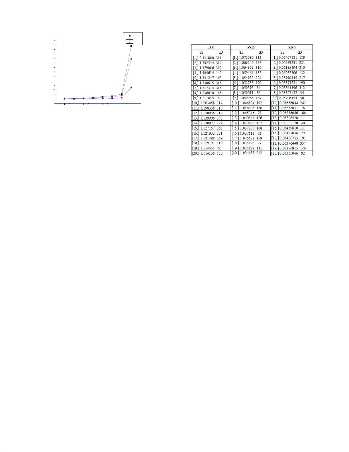
Finding rare information hidden in a huge amount of data from the Internet is a necessary but complex issue. Many researchers have studied this issue and have found effective methods to detect anomaly data in low dimensional space. However, as the di…
Authors: Zhana Bao
k- NS : Section - Based O utlier D etection in High Dimensional Spac e Zhana ABSTRACT Finding rare information hidden in a huge amount of data from the I nternet is a necessar y but complex issue. Many researchers have studied this issue and have found effective m ethods to detect anomaly data in low dimension al s pace . However, as the dimension increase s , most of these ex ist ing methods perform poor ly in detecting outliers because of “high dim ensional curse ”. Even though some approaches aim to solve this problem in high dimension al s pace, they can only detect some an omaly dat a appear ing in lo w dimension al s p ace and cannot detect all of anomaly data which appear different ly in high dimension al s pace . To cope with th is problem, we propos e a new k - nearest se ction - based method ( k- NS ) i n a section - based space. Our proposed approach n ot only detec ts outliers in low dimension al space with section - density rati o but also detec ts outliers in high dimension al space with the ratio of k- neares t section against average v alue . After taking a series of experiments with the dimension from 10 to 10000, the experiment results show that our proposed me thod achieve s 100% precision and 100% recall result in the case of extremely high dimension al s pace , and better improvement in low dimension al s pace compared to our previous ly proposed method. Categories and Subject D escriptors H .2.8 [ Data base Management ] : Database App lications - Data mining. I.5.3 [Pattern Recogn ition]: Ou tlier Detection. General Terms Algorithms, Experimentation, Performance Keywords Anomaly detection, Outlier detection, High dimension, Data projection, k - NS . 1. INTRODUCTION Seeking for meaningful information from very large database is alw ays a significant issue in data mining field . These valued dat a are called anomaly data , whic h are different from the rest of normal data based on some measures. They are also calle d outliers from a distance or density view . Many definitions about outliers are proposed according to different perspec tive s . The wi dely accepted definition about outlier is Hawkins’ : an outlier is an observation that deviates so much from other o bservations as to arouse suspicion that it was generated by a different mec hanism [7]. T his definition not only describes the difference of data from observation, but also point s out the essential di fference of data in mechanism . In the low dimension al s pace , outliers can be considered as far points from the normal point s base d on the distance. However, in high dimensional s pace, the d istanc e doesn’t meet the exact description between the anomaly data and normal data any longer. The only distinguished point is the differen ce in distributions between normal data and a nomaly da ta. Most of existing methods insist on finding the outliers by distance even in hi gh dimensional space. They can find anomaly data obviously far from normal data, but ignore the anomaly dat a that are inside the range of norm al data . Therefore, we give a new definition about a nomaly data i n high dimensional space in our approach : “ m ost of the data conform to one distribution such as the n ormal distribution, while the small pa rt of data conforms to another different distribution or just distribute random ly. T hese rare data are call ed anomal y data and only can be detec ted by some speci fic measures ”. In this paper, we reconsider the concept of outliers, explain the section spac e concept , and then propose a new algorithm called k- NS . The main features and contributions of this paper are summarized as follows : - We a nalyze the connection of d ata distribution bet ween the different dimensions . By this, the high dimensional problem is transformed in to the dimension al - loop problem. This problem is easi ly sol ved by some statistic method. - Our proposed method use s the k - NN (k Nearest Neighbor ) concept for the section calculation and put s forward to a novel k- NS (k N earest S ections) concept . Hence , o ur proposal can better evalu ate the disp erse degree of point s with neighbor points projected in a new dimension. - We rec onsider the concept of outlier, and employ section space instead of trad itional space in orde r to a void t he “ high dimensional curse ” problem. - We execute a series of experiments with the range of dimensions from 10 to 10000 to evaluate our p roposed algorithm. The experiment resul t s clearly show that our proposed algorithm has significant advantages ove r other algorithms with stably and precise ly in large volumes of dat a when the dimension increases extreme ly high. Even in the 10,000 dimensional data experiment , our algorithm easily achieves 100% precision and 100% reca ll result compared with ever - proposed anomaly detection algorithms. - We also point out the difference between the outliers and noisy data. The o utliers are obviously different in high dimensional space with n oisy data . These two concepts ar e confusing because the y are mixed together in low dim ension al s pace and even consider ed as identical by s ome resear chers . - Furthermore, we analyze the feature of data distribution in high dimensional space. Th e study on high dimensional space provides a new view to solve the a nomaly data detection issue. This paper is organized as follows . In section 2, we give a brief overview of related works on high dimensio nal outlier detection. In section 3, we introduce our concept a nd our novel approach, and we als o describe our proposal and discuss some optimizations. In section 4 , we evaluate the pr oposed method by experiments of Permission to make digital or hard copies of all or part of th is work for personal or classro om use is granted without fee prov ided that copies ar e not made or distrib uted for profit or commercial ad vantage and that copies bear this notice and th e full citation on the first pag e. To copy otherwise, or repub lish, to post on servers or to redistribute to lists, requires prior specific p ermission and/or a fee. Noname manuscript No. paper draft in 2012 different dimensional artificial data set and real dataset . And we conclude the findings in section 5. 2. RELATED WORKS As a n important sub - tree of the data mining field , anomaly data detection has been developed for more than ten years, and ma ny stud y results have been achieved in large scale da taba se . We categorize them into the following f ive groups to introduce these methods clearly . Distance a nd Density Based Outlie r Detection: The distance base d outlier detection is a classic method be cause it comes from the original outlier definition, i.e. Outliers are those points that are far from other po ints b ased on dis tance meas ures, e .g. by Hilout[ 8] . This algorithm detects point with its k - nearest neighbors by distance and use s space - filling curve to map high dimension al s pace . The most well -known LO F [ 1 ] uses k- NN and density based algorithm , w hich detect s the outlier locally by its k - nearest distance neighbor points and measure s outliers by lrd (local r eachabi lity de nsity ) and LOF (Local Outlier Factor ). This algorithm runs smoothly in low dimension al space and is still effective in relative high dim ensional space. LOCI [9] is an improved algorithm based on LOF, which is more sensitive to local di stanc e than LOF . However , LOCI perform s worse than LOF in high dimensional space. Subspace C lus tering Bas ed Outlier Detection: Since it is difficult to find outlier s in high dimensional space, they try to find these point s behaving abnormal ly in low dimension al s pa ce . Subspace clustering is a feasible me thod a pplie d to outlier detection in high dimension al s pace. This appr oach assumes that outliers are al ways deviated from others in low dimension al s pace if they are different in high dimension al s pace . Aggarwal [2] uses the e qui - depth ranges in each dimension with expec ted fraction and deviation of points in k -dim ensional cube D given by k f N × and ) 1 ( k k f f N − × × . This method detects outl iers by calculating the sparse coefficient S( D) of the cube D . Outlier D etection with Dimension D e duction : Another method is dimension deduction from high dimension al s pace to low dimension al space , su ch as SOM (Self - Organizing Map) [18 ] [ 19 ] , mapping sev eral dimensions to two dimensions, and then detecting the outlier s in two dimensional space. FindOut [ 11 ] detects outli er s by removing t he clusters and deducts dimension s with wavelet transform on multidimensional data. H owever, t his metho d may cause information loss when the dimension is reduc ed. The resu lt is not as robust as expected, and then it is seldom applied to outlier detection. Information- theory based O utlier Detection: The distribution of points in each dimension can be coded for data compression , hence high dimensional issue change s to information statistic issue in each dimension. Christian Bohm has proposed CoCo [3] method with MDL(Minimum Description Length) for outlier detection , and he also applies t his method to the cluster ing issue , e.g. Robust Information - theory Clustering[ 5][12]. Other Outlier D etection Methods: Beside s abov e four group s, some detect ion measurements a re also distinctive and useful. One notable a pproach is called ABOD ( Angle- Based Outlier Detectio n ) [4 ]. It is based on the concept of angle with vector product and scalar product. The outlier s usual ly have the sm all er angles tha n normal points. These methods have reduced the “ h igh dimensional cures” moderately a nd get the correct r esults in some speci al case s. However, “ high dimensional cur se ” problem still exist s a nd affects the point ’s detection . Christian Bohm’s inform ation -based method is similar to the subspace clustering methods and is only applied to detect outliers in low dimensional space. In summary , seeking a general approac h to detect outliers in h igh dimension al s pace is still a key issu e that n eeds to be solved. 3. PROPOSED METHO D It is well known that Euclidean distance between points in high dimensional sp ace become s obscure and immeasurab le . That is why there is “h igh dimensional curse ”. Moreover, o utlier detection in s ubspace or dimension reduction may ca use the information lost or only valid on specific datase t. We still need to find a suitable way for outlier detection in high dimensional space. 3.1 General Idea Learning from the subspace outlier de tection methods, we know that high dimensional issue c an be transform ed in to the statistic al issue by loop detection in different subspace s . We ha ve also noticed that points ’ positions change diffe rent ly in different dimensions. By observation and ana lysis of these points, we have found that t he outliers are placed in a big cluster of normal points in some dimensions and deviate d from these points in other dimensions. Otherwi se in another situation , the outlie rs are cluster ed different ly in different dimensions from normal points w hile normal poi nts are always cluster ed together in all dimensions. There fore , our proposed method only need s to solve the issue with two conditions: whether the re are points with low density in low dimensional space; or whether there are points that are deviat e d fro m other points in the same section of one dimension when the se points are projected to other dimensions. Our proposal can be divided into four steps . First, we divide the entire range of data into smal l regions in each dimension. Here , we ca ll th e small region a section . Based on the section divisions, w e construct the new data structure called section space , which is different from traditional Euclidean space. Second, we compare point ’s scatter ing with others in different section s in each dimension by co mputing t he section density value . Third, we compare the point ’s dispe rsing in the same section of one dimension after projecting it t o othe r dimensions . L ast, we sum u p all result s for each point, and then compare these points with a statistic meas ure. The outliers are th e points whose value s ar e obvious ly higher than most of the points . 3.2 Section Data Structur e O ur proposed method is ba sed on th e section data structure . The mechanism on how to c ompose this section structure and transform the Euclidean dat a space into our proposed section space is neces sarily introduced in detail in below. We d ivide the sp ace into the same number of sections in ea ch dimension, so the space just look s l ike a grid. The conventional data space i nformation is composed of point s and dimension s while o ur proposed data structur e represent s the data distribution with point, dimension and section . This structure overcome s the shortcomings of distance measurement i n conventional space, and it is easy to obs erve the distribution cha nges of points in one section wh ile section s and dimension s are varied in different situation s. The data structure is described by th e PointInfo ( point information) and SectionInfo ( section information ) as follows: An example of two dimensional data to explain t he transform ing process from original dataset to a new sect ion space is shown in Figure 1 . The example dataset include s 23 points in two dimensions as shown in Figure 1 (a). The original d ata are p laced in to the data space as in the conventional method, as shown in F igure 1(b). In our proposed section - based st ructure, we construct the PointInfo structure as illustrated in Figure 1(c) and S ection Info a s shown in Figure 1(d). The range of each dimension is divided into five sections. The section division sampl e is shown in data spa ce with blue lines as in Figure 1(b) and S ection I nfo as in Figure 1(d). We notice that the range of each dim ension is different. If we set the largest range for all dimensions , there must be too m any blank sections in the small range dimensions and the blank section s produce mean ingless values 0 would affect the result ma rkedly in fo llo wing calculations. Therefor e, we set the range from minimum coordinate to the maximum coordinate for each dimension . In order t o avoi d two end sections having larger density t han that of other sections, we loose the border by enlarge the origi n al ra nge by 0.1%. T ak i ng the data in F i gure 1 as an example to explain how to generate the range of the data in each dimension . T he original range in x dimension is (5, 23) , and the length is 18 . The new range is (4.991, 23. 009) by enlarging t he len gth by 0.1% , therefore, t he new length is18. 018. T he original range in y dimension is (6, 25) , and the length is 19 . The new rang e is (5.9905 , 25.009 5) , and the new length is 19.019 . The l ength of section is 3.6036 in x dim ension and 3.8038 in y dimension. 3.3 Definitions To provide an explicit explanation for our proposed method , some definitions are formulated as follows: Symbol Definition P (point) The information of point. p j refers to the j th point of all points. p i, j refers to the j th point in i th dimension. Section (section) The range of data in each dim ension i s divided into the same number of equ i - width parts, which are called section s. The width of the section is determined by the section density and the range in that dimension. s cn (number of section ) The number of sections for each dimension. It is decided by the number of total points and the average section den sity . scn is defined equally in each dimension. d ( section density) The number of points in one section is calle d section density. d i means the average section density in i th dimension. d i,j means the j th section den sity o f i th dimension. d i (p) mea ns the section dens ity of the point p to in i th dimension. d ist s (section distance) The section distance used for evaluating the section difference among points in all projected dimensions , a s defined in Equation (4). Sec Val (point section value) A point deviation value in each dimension as defined in Equation ( 3). SecValp (projected point section value) A point de viation value in project ed dimensions as defin ed in Equation ( 5). SI (statistic information) The statistic info rmation of e ach point as defined in Equation ( 6). d is the section density, which present s different meaning s in different cas es. Case1: i n one section, all points of this section have the s ame sectio n density , and d i, j means sectio n density value in the i th dimension a nd j th section. All poin ts in this section of dimension i have th e same d i, j value. Case2: the s ection density is used to compare with the ave rage value in this dimension. So the low section density has a low ratio with the average section density in one dimension . d i means the average section densi ty in i th dimension. Case3: if t he section den sity of a point is needed, the expression should include the point. d i (p) means t he section density value of point p in i th dimension. From above on, different subscriptions express a specific meaning for point, section of dimension, al though they are all expressed by d . Dimension projection is a concept that needs to be clarified. Each point has its coordinate value i n different dimensions. All dimensions have the equal rela tion s. However, when we observe the change of points in different dimensions, we need to fix the po ints of the same section in a certain dimension at first, and then compare the distance change of these points in other different dimensions. The ini tial dimension is called original dimension , and the different dimensions are called pro jected dimension. It means that we project the points from the original dimension to the other dimensions. 3.4 k- NS The outli er detectio n method in section spac e is different from the method in a conventional dat a space. The existing method s such as t hose using distan ce and density among points cannot be applied in the section space dir ectly. In section s pace, e ach point gets the v alues in different sections and dimensions, and then al l PointInfo [ Dimension ID, Point ID ] : section ID of the point SectionInf o [Dimension ID, Section ID]: #points in the section Figure 1: Section Space Division an d Dimension Projection these values decide whether the points are out liers or not. We propose a novel method effe ctive in high dimensional space, called k -n ear est sectio ns or k- NS . This proposed method is a statistic al approach whic h detects ou tlier s in each dimension and the projected dimensions. Before we introduce k- NS d efinition, the dis ts (section distance) need t o be clarified in ad vance . It is noted that the sec tion distance defined in this paper is different from the general definition of distance. DEFINITION 1 ( dists of points) Let point , . , are in i th di mension. When , are projected from dimension i to j, t he section distance between them corresponds to the difference of their section ID. (1) In ori ginal dimension i , p and q are in the same s ection. After th e dimension change from i to j , p a nd q have a new section ID. S o we can com pare the section difference between ) p ( SecId j and ) q ( SecId j . The dists is the absolute differen ce value between any two points. The minimum dists of point is 1, which is differen t from the conventional Euclidea n distance concept. Because the frequency of poi nts in the same secti on is more than that of points with the same coordinate , there must be many minimum sections distance. If all neighbor points have minimum dists 0 , the point gets value 0 from neighbor point ’s dists . In t his case , it easily cause illegal computation and invalid to compare with other points. So the minimum dis ts is s et 1 to solve this question perfect ly. The k- NS mat hematic definition is ba sed on the dists , which can find outliers in different situations. DEFINITION 2 (k- NS ) The x ns of a given point x in the database D is defined as } ) , ( ) , ' ( ) ( , , ' , , ' , 1 , 1 1 , 1 1 1 ∑ ∑ ∑ ∑ ∑ ∑ = ≠ = = ≠ = = = ≤ << ∈ ∈ ∀ ∈ = m i m i j j m i m i j j m i m i i i ns p x dists p x dists d x d Section p x x D x D x {x x (2) x , x` a nd p are th e points in the same sect ion in dimension i . The point p is any one of k- nearest points which give dists of neighbor points to compare it with othe r points from the original same section when project ing them to new dimensions. k- NS gives the effective method with dists t o discriminate the points of the same section by projecting the dimension from original to other s d. x ns is a statistic al value for summarizing all va lues of point in each dimension and in all projected dimension, which means the x ns could be use d a s a whole result finding outliers and impossible to be found in some certain dimensions. From the k-NS definition, outlier s should satisfy either of two conditions: The f irst con dition guarantee s tha t outliers can be detected in low dimensional space; t he second condition guarantees that outlier s still can be detected with neighbor points’ dists in the projected dim ensions if th e point does not appear abnormal in low dimensional space . Our proposed method use s loop calculation in dim ensions instead of the calculat ion of the Euclidean dis tance. The refore, each point needs to be evaluated in each dimension and each projected dimensions on first step . 1. Sectio n Density Rat io Comparison in Each Dime nsion Outlier point s alway s appear more sparsely than most normal points if they ca n be detected in low dimensions . Therefore, the density of outlier s is lower than the average density in that dimension. The section dens ity ratio of point s with the average section density doe s not only reflect the sparsity in the dimension, but also compare points between different dimensions. DEFINITION 3 (Section Density Ratio) Set point , , in dimension i , where j is point ID and k is section ID. d i,k is secti on densi ty of point , in dimension i and d i is the average section density in dimension i . T he point ’s SecVal in each dimension is defined as follows: (3) It is t o be noticed that SecVal is not the section densi ty value, but a r atio of the section density with the average value in that dimension. The reason is that a poi nt has different sparsity in different dimensions. If points only use section density to compare , the value is easi ly affected in dif ferent dimensions and cannot get accurate res ult . The ra tio of section density overcomes this shortcoming, which is independent among dimen sions and only decided by the distribution of the points in its own dimension. Another noticed a spect is that one SecVa l does not only correspond t o one point , but it actu ally pres ents the se ction’s density value. Hence the points which are in the same sec tion share the same SecVal values. 2: k- Nearest Section Comparison in Each Proj ected Dimensions If the outliers don’t appear farther in the low dimensions, they cannot be detected by the first step. Since they hide among the normal poi nts and have simil ar distance or density with others . Nevertheles s, these poin ts still ca n be found different from other po in ts in the same section in the projected dimension s . This step aims to find outliers from normal points by project ing t hese points into different dimensions. The section distance meas urement is a effective method to compare these points. Based on the section distance concept and referring to the k -N ear est Neighbor concept [10] , we can get the ratio of the nearest sect ion s of the point in the projected dimensions. DEFINITION 4 (Nearest Sections in projected dimension ) Set point , , and project dimension i to k , where , . q is ’s any k- nearest neighbor point s. f , k p is the point wh ere f , i p and , are in the same section . s is the number of points in the same section with , . Then SecValp of point , is defined as follows: (4) We calculate the ’s dists with k- ne arest neighbor points, and then ge t the ratio value with average value of points’ d ist s in t he section in the original dimension . Whi le the dimension is projected to another dimension , it gets one SecValp value each 2 = i i,k i,j d d ) SecVal(p 2 1 , 2 , , ) ) , ( 1 ) , ( ) , ( ∑ = = s f f k j k j i q p dists s q) p dists k p SecValp 1 ) ( ) ( ) , ( + − = j j i i q SecId p SecId q p dists time of projection . Totally, it gets m × (m- 1) Sec Valp values from all the projected dimensions for each point. 3. S tatistic al Inform ation Values for Each Point Through the above two steps calculation , each point gets m SecVal values in each dimension and gets m × (m - 1) SecValp values in all the proj ected dimensions. We give the general statistic al approach for e ach point p i in the section s pace, which is shown in Definition ( 5). DEFINITION 5 (Statistic al Information of Point ) Set SecVal(p k ) is the value of p k in each dimension, and SecValp(p k ) is the value of p k in all projected dimensions. and are the weight for SecVal and SecValp . Then the statistic al information value of p i is calculated as follows: (5) SI (Statistic Information) is the point ’s value which is distinct among different points, and the outlier’s SI value is obviously different from normal point ’s value. For the different dataset, changing the weight values coul d bring the better result. However, here, we use weight = and = ( ) for clearly clarifying the SI. The effective statisti c method is consider ed i n order to give the sharp boundary to compare with other points. By eva luat ing different methods and the ir performance, w e choose a simple a nd clear calculat ion method . Here, w e get the re ciprocal value of average SecVal and SecValp . T he outliers have obviousl y larger SI (Statistic al Inform ation) than that of the normal points’ . DEFINITION 6 (Statistic Information of point) (6) This equation simply sums up SecVal and SecValp in all dimensions. Whether getting point ’s value in each dimension or in projected dimensions, all these point ’s values are the rati o with the average va lue i n their respective dimensions . Most of the time normal points are around the average value in the dimension. Hence th e SI value for normal points should be close to 1, and outlier’s SI value should obviously larger than 1. However, it is not tru e in high dimensional space. Normal points’ SI are get ting smaller with the dimension increasing, and their values are always much lower than 1 , as well as the outlier’s values are also lowe r than 1. Neverthel ess , the outlier’s SI is still obviously high er than normal points’ . Therefore, o utlier s can be easily found just by to sort ing points by the ir SI values . 3.5 Algorithm In t his section , we focus on how to implem ent the k- NS me thod in R language. How to ge t PointInfo an d SectionI nfo effectively in different sections and dimensions is k ey issue that needs to be considered in detail. T he proposed algorithm is shown in Figure 2 with pseudo - R code . Set the data set contain ing n points with m dimension. The range of dat a is divided into scn sections in each dimension. Figure 2: k-NS Algorithm Algorithm: k- Nearest Section Input: k, data[n,m], scn Begin Initialize(PointInfo [n, m], SectionInfo[scn, m] ) For i=1 to m d i =n/length(SectionInfo[ SectionInfo[i,]!=0 ,i] ) For j=1 t o n Get Pt Val 1 [i,j] with Defi nition (3) End n End m For c =1 to 5 Random sort dimension i For i=1 to m F or j= 1 to sc n Pt Num <- SecInfo[j,i] If( PtNum == 0) next Ptid < - which(PtInfo[,i]==j) If( PtNum < × ) SecValp =1 else For each(p in Ptid ]) { if ( i> SI or top SI) Three points need to be clarified in this algorithm . The f irst point is how to de cide the average section density d i in each dim ension . d i value is easily obt ai ned from calculation , which is the definition of the average section density . It means d i is s ame in each dimens ion. However, in the case that most points dis tribute in some small part s of sections a nd no point exist s in other sections , d i becomes very low and even close to the outlier ’ s section density. So , we only count section s with point s , but don’t count the section s without points for ca lcula ting d i . Subsequently, d i reflects the average section density of points in i th dimension, but i t also vari es in different dimensions. Hence, the ratio of the section density to d i in Definition (3) can measure the sparsity of points in different sections in a dimension . ∑ ∑ = − = × − + = m 1 i 1 m 1 k 2 j , i 2 j i, j ) ) k , SecValp(p 1 m 1 ) (SecVal(p m 2 ) SI(p ) ) p ( SecValp ( ) ) p ( SecVal ( ) p ( SI m 1 i m i j , 1 j k 2 m 1 i k 1 k ∑ ∑ ∑ = ≠ = = + = ω ω The s econd point is about the number of dimension loop in calculatin g all the point projections . For any point in a certain dimension, it can be projected to other (m -1) dimensions. Hence , the total dimension loops can be × ( 1) . However, the calculation cost of th e all dimension loops i s t oo e xpensive since the algorithm is applied to high dim ension al space . Through the plenty of experiments, we have found that the number of projected dimension loop could be expressed by × ( 1 ( 1) , and t he proposed value for is 5 where the projected dimension should be sorte d by random order. Then t he projected dimension s can be visited by th e order from 1 to 2, 2 to 3, … , m to 1. The total dimension lo op number is 5 × with a little accuracy loss , but it reduced the computing time g reatly. T he t hird point is the number of points in one section. The re are three different cases . Case 1: no point in the se ction. In this cas e, t he algorithm just passes this section and goes to the next section. Case 2: man y points in the s ection. In t his case, the neares t section method is ju st used to detect points. Ca se 3: only a few points i n the section. In this case , t he point distribution is difficult to be judged just by these several points. And the sect ion density ratio in the step 1 must b e very l ow. Therefore, these points are to be already det ected by the p revious s tep. Here , we se t t he SecValp =1. The threshold value to sep arate the case 2 and case 3 is related to the k . k should not be large because k is less than d i in the projection dimension in the step 2. Through ex periments wi th a serious of value s from 4 to 20 to find the suitable va lue for k and the threshold of t he number of points in one section , w e have found that the threshold value can be defined as × as t he best solution which could be adapted in most of the situations. 3.6 Distinction betw een Outliers and Noisy Data The concept of outlier and noisy data has been p roposed for more than ten years . According to that, o utlier is regarded as abnormal data which is gene rated by a different me chanism and contain s very important information , and n oisy dat a are reg arded as a s ide product of clustering points, which have no useful information but affect the correct resu lt grea tly . In the data space, the outliers are points that are farther from others by some measures, while the noisy points alway s appear around the outliers. Since the noi sy points are also far away from the normal points , i n low dimension al s pace , it is difficult to make a dis tinct boundar y betwe en out liers and noisy points . Bas ed on these frustrated observations, s om e researchers even consider that noisy data as a kind of outliers. There is no difference in detecting abnormal data by any methods. Hence, it is a meaningful issue to make a distinction between outlier s and noisy points not only in concept but also in detection measures. In this paper, we try to explain the di stinction between outliers and noisy points in two aspec ts. The f irst point is that there are different data genera tion proces ses. Outli ers are gen erated b y a different distribution from norm al points. Noisy points have the same distribution with normal points. The s econd point is that they appear abnormal i n different dimensiona l s pace . Noisy points only appear abnormal ly in several dimensions and appear normal in other dimensions. From the whole dimensions ’ view , th ese noisy data also conform to the same distributio n of normal data. The outlier may appear in the same way in low dimension al s pace , but they conform to di fferent distribution mechanism from nor mal points’. Therefore, w e can get a conclusion from these points that both outliers and noisy points can be detected in low dimension al space, but only outliers can be found in high dim ensional space. An example of noi sy data sa mple is shown in Figure 3 . The data is retrieved from Dataset 8 as introduced in section 4, which contains 1000 points in 10000 dimensions. The outliers are p lace d in the middle region and can be found different ly from normal points. The noisy points are labeled with cloud that is so different in this projected two dimensional space. Another example is shown in Figure 4 . The outliers are not obvious in two - dimensional space, while noisy poi nts that distribute on the marginal area of both dimensions a re more likely abnormal points. 4. EVALUATIO N We have implemented our algorithm and appl ied it to several high dimensional datasets , and then have made the comparison among k- NS , LOF and our previous proposed methods. In order to compare these algorithms under fair c onditions, we perform ed all algorithms with R language, on a Mac Book P ro with 2.53GHz Intel core 2 CPU and 4G memor y. On the issue of outlier detection in high dimensional space, w e have proposed two algorithms , called RPGS (Rim Projected Grid Statistic) [ 6 ] and PSD (Projected Section Density ) [ under review] . RPGS is a statistic me thod that us es r atio of section density in each dimens ion and c enter section function in projected dimensions. The key definition about Center Section Function is shown in D efinition 7. RPGS is only effective in one cluster data distribution in high dimensional space and cannot work well in more than two clustered data distributions . DEFINITION 7 (Center Section Function ) (7) (8) MinSec is the minimum section ID; MaxSec is the max imum section ID. I f SecID > Sec center , E quation(7 ) is used, or else Equation ( 8 ) is used. PSD is a nother proposed algorithm which detects outliers effect ively in ver y high dimensional space. PSD is quit e similar to k- NS algorithm, and it also includes the three - step detection method . PSD ’s peculia rity is on the second step for estimating outliers in projected dimension, which employ s a new sec tion - Figure 3: Noisy Data of Dataset 3 Projected to Two - Di mensional Spa ce center center i i 2 Sec MaxSec Sec ) x ( SecID ) x ( PtVal − − = MinSec Sec ) x ( SecID Sec ) x ( PtVal center i center i 2 − − = cluster concep t, and calculat e the ratio of s ection - cluster density to the mean value of points in the section. The calcu lation of section - cluster in PSD is shown in Definition ( 8 ). DEFINITION 8 (Section- cluster) (9) Where the CluLe n j is the cluster length according to the section of p j in k dimension, Sec(p k, j ) is the number of points in the section where the point p j is projected in k th dimension from i th dimension by changing k , and s is the number of points in the same section of p i,j . The denominator is the average value of the points by the product of Sec and the CluLen in dimension k . Compared with RPGS, PSD is an improved algorithm which can detect outlier in the case of different data distributions. In this paper, the normal points of te st datas et conform to five clusters of Gaussian mixture model. RPGS performs poorly in the experiments. Therefore, we only show the experiment result of LOF, PSD and k- NS . 4.1 Synthetic Data set A critical issue of evaluating outlier detection al gorithms is that no benchmark dataset s h ave be en found in real world to satisf y the explici t division between outlier s and normal points. The points that are found as outliers in some real datas et are impossible to provide a reason able explanation why t hese points are picked out as outliers . On the other hand, what we have learned from the statistical knowledge is helpful to generate the artificial dataset: if some points with some distribut ions are apparently different from those of normal points, the se points can be regarded as outliers . Hence , w e g enerate the synthetic dat a based on this assumption. Since o ur alg orithm aim s to solve the problem i n high dimension al s pace , w e g enerate the eight syntheti c dataset s with points of 500- 1000 and dimension s of 10-10000. The normal points conform to the n ormal distributions , while outliers conform to the random distributions in a fixed region . Norm al points are equal ly distributed in five clusters and 10 outlier s are distributed randomly in the middle of norm al points’ range. The more deta ils ab out the parameters in each dataset are shown in Table 1 . Table 1 : Synthetic Dataset The synthetic dat a sets are generat ed by the speci al rules t hat outliers ’ range should be within the range of the normal points in any dimensions. Therefore, outliers cannot be fo und in l ow dimension al space . The data distribution example is shown in Figure 4 where the D ataset 3 is projected to two -dimensional space with outlier s labeled with red col or . It is clearly shown in Figure 4 that the outliers are distributed within the range of normal poin ts and show no difference to the normal points in this two - dimensional space. Noisy points th at are placed on the margin of distribu ted area ar e more lik ely regarde d as abnormal points. Hence, the differen t distributions for outliers and normal data cannot be found just by the str aight observation. The outliers are designed to be loosely distributed, and they may be scattered further out of some fixed regions with small probability. Nevertheless these outliers are still within the range of normal points. 4.2 Effectiveness In this subsection, our proposed algorithms is evaluated thoroughly by a series of exper iments and compared with LOF and our previous proposed methods . In order to measure the performance of these algorithms to find most likely outliers at least fal se ra te , the 10 outliers are reprieved one by one. Therefore , it could provide the clear figures t hat describe the effectiveness of points are checke d out on any extent of founde d detected outli ers. In the case of 10 dimensional dataset test, w e us e the precision and t he recall for the better measurem ent of outlier detection efficiency among three algorithms. Since the recall is the percentage o f all outliers in the data set tha t have been found correctly , the 10 precision figures clearly show the t rend on how effective ly the outliers could be identified from all attained points. To contrast with the result affect ed by increasing the dimension from 10 to 100, we also use the precision and th e reca ll measuremen t to evaluate the e xperiment results in the D ataset 2. In the processing of all eight dataset experim ents, we evaluate th e performance of the algorithm s with F - measu re by increasing dimension from 10 to 10000. In each dataset experiment , we obt ained 10 precisions and t he ten recall results respectiv ely. Then the 10 F- measure v alues ar e obtai ned for each dataset test. We pick up the best F - measure from each datas et f or bette r demonstrating the experiment performance by LOF, PSD and k- NS . At the beginning , we need to set all the appropriate parameters for the three algorithm s in eight experimental data set s , as shown in Table 2 . The parameters shown in this table are the best ones for the prepar ed datasets , and the y may changed according to the si ze of data, the number of dimension s , etc . The parameter K nn of ∑ = × × = s 1 f f f , k j j , k j , i CluLen ) p ( Sec s 1 CluLen ) Sec(p ) k , p ( SecValp Figure 4: Data set 3 Projected to T wo - Dimensional Spa ce LOF is not set as a large val ue in a ll experiments because the dataset size is only around 500 or 1000 points. This is a reasonable ra tio of neighbor points ag ainst the whole dataset size. For PSD algorithm, the parameters of dst a nd scn are inverse each other. The product of dst and scn is almost equal to the total poin ts number . We set scn a little larger than dst because thes e combinations of parameters have shown the be tter experiment re sult s. The parameters of k- NS ar e set similar to the previous two algorithms and are verified as applicable in all experiments. Table 2: Parameters of LOF, PSD and k- NS Since in our dataset design, the outliers are placed inside the range of no r mal data to prevent these points easi ly to be found in low dimension al s pace . For this reason , it is difficu lt to find exact outliers in 10 dimension al s pace . The 10 dimensional experiment result is shown in Figure 5 (a) . LOF performs best in this 10 - dimensional test . Especially LOF can detect two out liers with very high precision. Nevertheles s, the pr ecision of LOF fall s down sharply with the increasing recall from 20% to 40 % . At l ast, the result of precision is worst among the three a lgorithms in detecting all ou tlier s correctly. k- NS synthesize two algorithms ’ advantage , and t he performance of k- NS i s bet ween LOF and PSD . To be noticed, the k - NS’s precision is always higher than PSD at any recall r ate. We can get the conclusion from the ex periment result as s een in Figure 5 (a) , t he LOF get s high precision with lo w recall, get s low precision with high recall, and get s the worst precision with 100% recall. Both PSD and k- NS get low precision in lo w recall; get lower precision with the incr eased recall. The k - NS achieves double precision better than PSD’s in low recall, and still better with increas ed recall . When the number of dimension increase s to 100 , the precision and recall evaluation in 2 nd dataset are clearly s hown the effectiveness of three algorithms. Distinctly from the first dataset , both PSD and k- NS achieve the 100% precision with any recall all the time . LOF obviously reduces the precision from 100% to 43.48% with the increasing reca ll from 7 0% to 100% , a s shown in Figure 5(b). In fact, P SD and k- NS keep t he perfect re sult in 1 00 dimension s, while LOF perform s much poorer with increasing t he number of dimension s in terms of the precision and the recall . To show the whole results of the effectiveness of three algorithms in all datasets with different nu mber of dimensions, we also use the F - measure in e ach dataset . The F - measure can provide a more clear an d simple evaluation in dex tha n the precision and the rec all to contrast LOF , PSD and k- NS in different datasets. In the experiment of d ataset s from 1 to 8, we evaluate the effectiven ess for three algorithms as shown in F igure 5(c) . LOF only achieves the b est F- measu re for each dataset , while PSD and k- NS only need to pick t he largest F -measure in the first dataset. Since F - measures are al ways 1 from the D atasets 2 to 8 . It is clearly shown that PSD and k- NS perform perfe ctly in the number of dimensions from 100 to 10000 w hile LOF only work s well in around 100 dimensional dataset . With the dimension increasing , LOF suffers th e high dimensional curse greatly , and F- measure of LOF are less than 0.2 in the dataset 4 -8. Learn ing from the dataset size test in Dataset 2 and 3 , the three algorithms get better ac curacy with the increasi ng dataset s ize . 4.3 Efficiencie s In this subsection , we compare three algorithms in runni ng- time. In R language, the running time include s user time , system t ime and total time. So we only use the user time to compare them. As shown in Figure 6, LOF i s the fastest algorithm in all experiments. PSD ru ns a little fa ster than k- NS . The averag e running- time of K- NS is 1.51 times of PSD, and 6.65 times of LOF. The three a lgorithms take more time w hen the number of dimensions increases or the data size is en larged. The reason is that there is no dimension -loop calculation for LOF because i t only processes the distance bet ween a point and its neighbors. However, our proposed algorithms PSD and k- NS both calculate values in all dimensions and in all different projected dimensions. Because k- NS gets calculation on neighbor points around a point, it takes more time to process than PSD. 4.4 Performance on Real World Data In this subsection, we compare the three algorithm s with a real - world dataset p ublicly avail able at the UCI machine le arning 0 1 2 3 4 5 6 7 8 9 0.0 0.2 0.4 0.6 0.8 1.0 F-measure Dataset LOF PSD k- NS (c) F - measure of Dataset 1 -8 0.0 0.2 0.4 0.6 0.8 1.0 0.0 0.2 0.4 0.6 0.8 1.0 Preci si on Recall LOF PSD k-NS 0.0 0.2 0.4 0.6 0.8 1.0 0.4 0.5 0.6 0.7 0.8 0.9 1.0 Preci si on Recall LOF PSD k-NS (a) Precision - Recall in 10 Dimensions (b) Precision - Recall in 100 Dimensions Figure 5: Effectiveness Comparison with LOF, PSD and k - N S in Eight Synthetic Datasets. Precision - Recall in 10 Dime nsions and 100 Dime nsions. F - measure Evaluation in Eight Datasets repository. ( h ttp://archiv e.ics.uci .edu/ml/dat asets/Ar cene ). We use Arcene dataset which is provided by ARCECE group. The task of the group is to distinguish cancer versus normal patterns from mass - spectrom etric data. Th is is a tw o - class classification problem with continuous input variables. This dataset is one of five data sets from the NIPS 2003 feature selection challenge. The ori ginal dataset includes tota l 900 instances with 10000 attributes. The dataset s have training datas et, validating dataset and test datas et. Each s ub - dataset is labeled with positive a nd negative. In order to compare the a lgorithms clearly without distraction by u nn ecessary data , we only pick up positive test dataset (310 instances ) as an eval uation targ et. In the dataset, there are no true labeled outliers. Therefore, we evaluate the r esults with th e top 20 value points, an d try to f ind the number of the same poin ts in th e se top 20 points. The experiment al resul t is shown i n Table 3 . T he only one point (ID 310) i s commonly det ected by th e three algorithms. The PSD and k- NS detec t the common 16 points in the ir top 20 points , w hile LOF detect s 19 diffe rent points . One possible reason is that PSD and k- NS use t he same section - space framework while LOF uses the neighbor points ’ distance. Another possible reason is that LOF run s with poor performance in high dimension al space . The result also prove s that LOF can find outliers, but in a limited w ay. 5. CONCLUSTIO NS In this paper, we introduce a new outlier detection m ethod, called k- NS , being de signed to effi ciently d etect out liers in a large and high dimensional dataset. The basic idea is t he three- step statistic al met hod , which (i ) calculates the sectio n density rati o in each dimension; ( ii ) computes the nearest se ction s ratio in all projected dimensions , a nd ( iii ) summarizes all valu es of each point for comparison with those of the other points . Our proposed k- NS algorithm has the following advantages : Imm une to the high dimensional curse, Adapt to various outlier distributions, And outstanding performance in large scale dat a set of high dimensional data space . In the experimental evaluation we have demonstrated that k- NS performs significantly better than PSD in low dimension al s pace , achieve s equal ly excellent r esult s in high dimension al s pace . We also provide evidence of its effectiven ess as compared with LO F in high dimensional space. The difference between outliers and noisy data is also discussed in this paper. This issue is difficult to be solved in low dimension al s pace since both data are always mixed together. In our experiments, the noisy data can be separated from outliers by project ing points from high dimensional space to two -dimensional space. The interesting point is that noi sy data seem mo re abnormal than outliers in projected low dimensional space. As the ongoing and future work, we continue to design and improve the algorithms under the section - space framework . More experiments need to be tested in order to seek for the perfect solution in outlier detection in high dimensional space. Another issue is the expensive cost of processing time in hig h dimensional data tests. Any solution to reduce the processing time ne ed s to be investigated. One of the approaches may be the use of the parallel processing. This k- NS method can also be applied to other data mining technology such as clu ster ing in high dimensions , classificat ions , etc. 6. REFERENCES [1] Markus M.Breunig, Hans - Peter Kriegel, Ra ymond T.Ng, Jorg Sander. LOF : Indetify density - based local outliers . Proceedings of the 2000 ACM SIGMOD international conference on Management of data . [2] Charu C.Aggarwal, Philip S.Yu. Outlier detection for high dimensional data . Proceedings of the 2001 ACM SIGMOD international conference on Management of data . [3] Christian Bohm, Katrin Haegler. CoCo: coding cost for parameter - fr ee outlier de tection. In Proce edings of the 15th ACM SIGKDD international conference on Knowledge discovery and data mining. 2009. [4] Hans - peter Kriegel, Matthias Schubert, Arthur Zimek. Angle- based outlier detection in high dimensional data. The 14th ACM SIGKDD international conference on Knowledge discovery and data mining . 2008. [5] Christian Bohm, Christos Faloutsos, etc. Robust information theoretic clustering. The 12th ACM SIGKDD intern ational conference on Knowledge discovery and data mining. 2006. [6] Zhana , Wa taru Kamey ama. A Proposal for Outlier De tection in High Dimensional Space. The 73 rd National Convention of Information Processing Society of Japan, 2011. Table 3: Top 20 points of arcane data Figure 6: Running Time 0 1 2 3 4 5 6 7 8 9 0 1000 2000 3000 4000 5000 6000 Time(Sec) Dataset LOF PSD k-NS [7] D. Hawkins. Identification of Outliers. Chapman and Hall, London, 1980. [8] Fabrizio Angiulli and Clara Pizzuti. Outlier mining in large high- dimensional d ata sets. IEEE Transactions on Knowledge and Data Engineering (TKDE), 17(2):203 -215, February 2005. [9] Spiros Papa dimitriou, Hiroyuki Kitagawa, Phillip B.Gibbons . LOCI: fast outlier detection using the local correlation integral. IEEE 19 th International conference on data engineering 2003. [10] Alexandar Hinnerburg, Charu C. aggarwal , Daniel A . Keim . What is the nearest neighbor in high dimensional space ? Proceedings of the 26th VLDB Conference, 2000. [11] Dantong Yu , etc. FindOut : finding outliers in very large datasets. Knowledge and Information System (2002) 4:387 - 412. [12] Christian Bohm, Christos Faloutsos, etc. Outlier -robu st clustering using independent compone nts. Proceedings of the 2008 ACM SIGMOD international conference on Management of data. [13] Das, K. and Sc hneider, J . Detecting anomalous records in categorical datasets . the 13th ACM SIGKDD international conference on Knowledge discovery and data mining, 2007. [14] Lance Parsons, Ehtesham H aque, Huan Liu . Subspac e clustering for high dimensional data: a r eview. ACM SIGKDD Explorations Newsletter. Volume 6 Issue 1, June 2004. [15] Lee, W. and Xi ang, D. Information - theoretic measures for anomaly d etection. I n Proceedings of the I EEE Symposium on Security and Privacy. IEEE Computer Soci ety, 2001. [16] Feng chen, Chang - Tien Lu, Arnold P. Boedihardjo. GLS - SOD: a gene ralized loca l statistical appr oac h for spatial outlier detection . . In Proceedings of the 16th ACM SIGKDD international conference on Knowledge discovery and d ata mining. 20 10. [17] Das, K. and Sc hneider, J . Detecting anomalous records in catego rical datase ts. . In Proceedings of the 13th A CM SIGKDD international conference on Knowledge discover y and data mining , 2007. [18] Ashok K. Nag, Am it Mitra, etc. Multiple outelier detection in multivariate data us ing self - organizing maps title . Computational statistics. 2005.20:245 -264. [19] Teuvo kohonen . The self -organizing ma p . Proceedings of the IEEE, Vol.78, No.9, September, 1990. [20] Moore, D. S. and McCabe , G. P. Introduction to the Pra ctice of Statistics, 3rd. New York: W. H. Freeman, 1999. [21] Naoki Abe , Bianca Zadrozn y , John Langford . Outlier Detection by Active Learning . Proceedings of the 12th ACM SIGKDD international conference on Knowledge discover y and data mining, 2006. [22] Ji Zhang, Qi ang Gao, et c. Detecting projected outliers in hig h dimensional data streams. In Proceedings of th e 20th International Conference on Database and Exp ert Systems Applications (DEXA '09). [23] Alexander Hinneburg, Daniel A. Keim . Optimal grid - clustering:Towards breaking the curse of dimensionality in high dimensional clustering. The 25 th VLDB conference 1999. [24] Aaron Ceglar, John F.Roddick and David M.W.Powers. CURIO: A fast outlier and outlier cluster detection algorithm for larger datasets . AIDM ' 07 Proceedings of the 2nd international workshop on Integrating artificial intelligence and data mining , Vol . 84 . Australia, 2007. [25] Pete r Filzmoser, Ricardo Maronna and Mark Werner. Outlier Identification in High Dimens ions. Compu tational Statist ics & Data Analy sis. V ol. 52 , 2008. [26] Amol Ghoti ng , etc. Fast Mining of Distance - Based Outliers in High - Dimensional Datas ets . Data M ining and Knowl e dge D iscovery. Vol .16:349-364 , 2008. [27] Shohei H ido, etc. Statistical outlier detection using direct density ratio estimation . Knowledge and Information Systems. vol.26 , no.2, pp.309 - 336, 2011 .
Original Paper
Loading high-quality paper...
Comments & Academic Discussion
Loading comments...
Leave a Comment