Robust Subspace Outlier Detection in High Dimensional Space

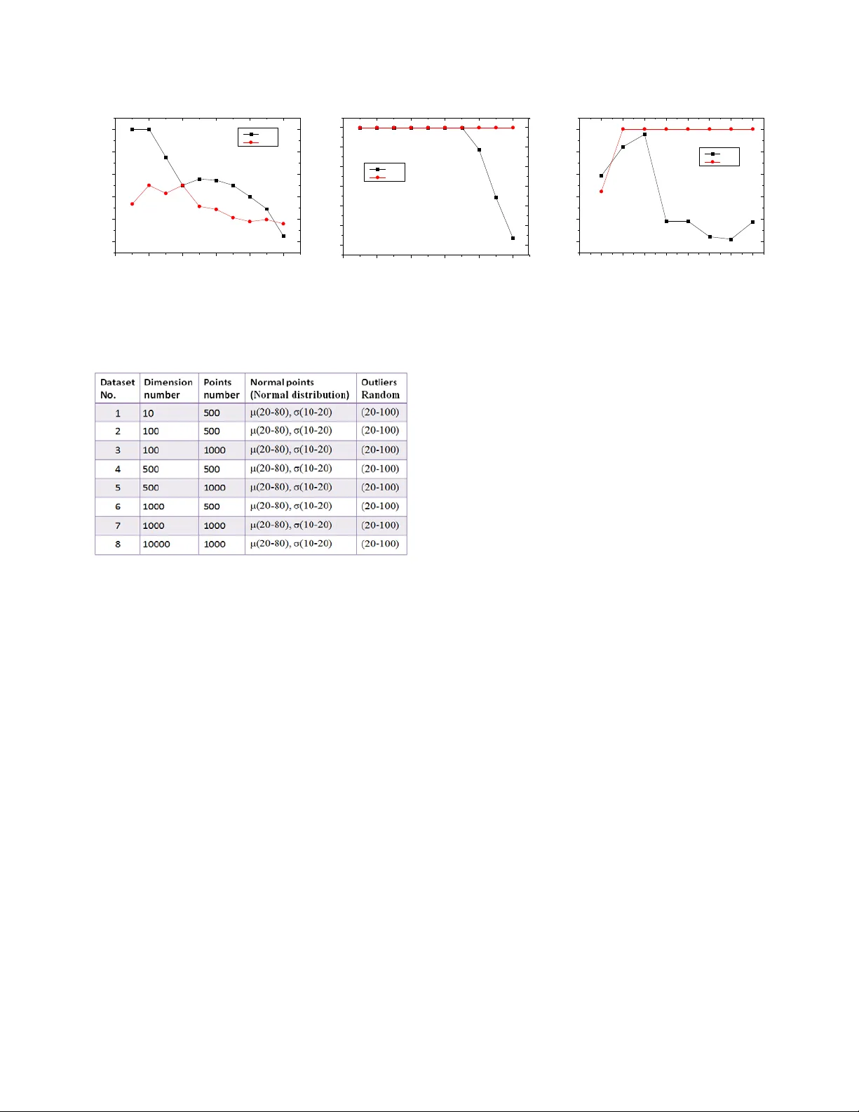
Robust Subspace O utlier Detecti on in High Dimensional Space Zhana Abstract —Rare data in a large- scale database are calle d outliers that reveal significant information in the real world. The subspace - bas ed outlier detection is regarded as a feasible approach in v ery high dimensional space . However, t he outlier s found in subspace s are only part of the true outliers in high dimensional space , i ndeed. The out liers hid den i n normal - clustered points are sometimes neglected in the projected dimensional subspace. In thi s paper, we propo se a robust subspace method for detecting such in ner outliers in a given dataset, which us es tw o dimensional -proje ctions : detect ing outlier s in subspace s w ith local density ratio in the first projected dimensions; find ing outliers by compari ng neighbor ’s positions in the second pr ojected di mensions. Each point’s weight is calcu lated by summing up all related values got in the two steps projected di mensions, a nd then the points scoring the largest weight values are taken as outliers. By taking a series of experiments with the number of dime nsion s from 10 to 10000, the results show that our proposed method achieves high precision in the case of extremely high dimensional space, and wor k s well in low dim ensional sp ace. Keywords- Outlier detection ; High dimens ional s ubspace; Dimension projection; k- NS ; I. I NTRODUCTION Finding ra re and valuab le data i s always a sign ificant issue in da ta mi ning field. These worthy d ata are called anomaly data that are different from the rest of the n ormal data based on some measures. They are al so called outlie rs that are lo cated far in distance from ot hers . O utlier detection has many practical applications in different domains , such as medicine developm ent, fraud de tection, sports statist ics analysis , public healt h managem ent, and so on . According to different perspectives, m any definitions about outlier s are proposed . The widely acc epted definit ion is Hawkins ’ : an outlier i s an observa tion that deviate s so muc h from other observati ons as t o arouse sus picion that it was g enerated by a different mechanism[7]. This definition not only desc ribes the difference o f data from obse rvation but also poi nts out the essential difference of data in mechan ism; even though some sy nthetic data are generated according to this conc ept in order t o verify their outliers’ detection met hod s. Although outlier detection itself does n ot h ave a special requireme nt for high di mension al space , large - scale data are mor e p racticable in the real world. T he re a re two issues for outlier de tecti on in high dim ensional s pace: the first on e is to overcom e the complexity in high dimension al s pace, and th e other is to meet the requirem ent for real applications with the tremendous growth of hi gh dime nsional data . In low dimensi onal space , outliers can be co nsidered a s far point s from the normal points based on the di stance. H owever, i n high dim ensi on al space, the distanc e no longer m eets the exact description b etween outliers and normal data. In th is case, detecting ou tliers falls into two categories , distance - based and s ubspace - based m ethods . The first one use s robust distance or densi ty in high dimensiona l space , i.e. LOF[1], Hilout[ 8], LOCI[3], GridLOF[1 4 ] , ABOD[ 4 ], etc. These methods a re suitabl e for the outl ier detection in not hig h dimensi onal space . However, in very high dimensiona l space, they perf orm poor because of “curse of dim e nsions”. T he other one that subsp ace based d etection is an optimum method t o find outl iers in high dimensiona l space. It is based on the assum ption that the outliers in al l low proj ected dimensi onal subspace s are taken as real outliers in hig h dimensional space. Th is solution i ncludes Agga rwal’s Fraction[ 2 ], GLS - SOD [1 6 ], CURIO [ 15 ], SP OT [ 22 ], Grid - Clustering[ 23 ], etc. Since outliers are easily found in low projecte d dimensi ons using som e optimize d search algorithm s to fi nd suitable cell - grid s that are division s of subspace, it is widely u sed for outlier detection in h igh dimensional space. Recent adv ance in geo - spatial, bio - informa tics, genet ics and pa rticle physics als o require m ore robust su bspace det ection m ethods in growing hi gh dimensi onal data. However, one key issue is still uncertain: - Is that truth tha t the ou tliers detected in subspac e s are all outliers in high dimensional space ? a. 3 - Dimension b. X- Y Dimensio n c. X- Z Dimension d. Y- Z Di mension Figure 1 . Sa mple data plotted in three - dimension al space and in two - dimensional spaces. Four red outliers s eparated in (a) are observed . But in (b), (c) an d (d), only two red outliers are ob served. Other two outliers are hidden in the no rmal clusters. Noname manuscript No. In 2012 I n fac t, subspace - based detection m ethods can find some outliers different fr om norm al points in projected dim e nsional space , but they i gnore the outliers hid den inside the region of normal data. These inne r o utliers are still different from norm al dat a in high dim ensional space. We show a simpl e ex a mp le to prove the difference between these two types of outliers separately in three - dimens ional s pace and projected two - dimensi onal subspace s , as shown in Fig . 1. Total 124 point s are distr ibute d in a thre e - dim ension al s pace , including 12 0 norm al point s in six cl usters a nd 4 ou tliers in red color. In (a) , four outliers c an be fo und differe ntly because they do not belong t o any normal clusters. T he outlier s O 3 and O 4 are detected different i n any of the projecte d dimensi on al s paces , w hile the inner outliers O 1 and O 2 are hid den inside the cluster s in the project ed dimensi on al s pace . Ther efore , detecting O 1 and O 2 fails . A ll subspac e - based m ethods fail to detect these inner ou tliers , as shown i n (b), (c) and (d) . Fr om the above, h o w to find all outliers with subspace - based m ethod is still an issue to be considered . In this pa per, we try to so lve t his issue by utilizin g the two dimension al - project ion s and propose a robust subspace detection method called k - NS(k - Nearest Sections). It calculates ldr ( local density ratio ) in th e first pr ojected dimensi onal subspace and th e nearest nei ghbors ’ ld r in the second pro jected di mensi onal subspace . Then , each point’s weight is su mmed statistically . The outliers are th ose scoring the largest weigh t s. The mai n features a nd contr ibutions o f this paper are s ummarized as follows: - We apply two dimens ional - projection s to calculate the weight val ues in all projected dimensi ons . For each poi nt, we supply the ( m m ( m 1) +× − ) weight value s in o rder to compare it with others e xtensivel y. - Our p roposed method employ s k - NS(k - Nearest Sections) based on the k - NN (k Neares t Neighbo r) concept for the local density calculation in th e second projected dime nsional spac e . The inner outliers are detected successfully by evaluating the neighbor ’s ldr aft er p rojecting them into other dime nsion s. - We execute a series of experiments with the range of dime nsions from 10 to 10000 t o eval uate our proposed algorithm. The experim ent result s show t hat our pro posed algorit hm has a dvanta ges ove r other a lgorit hms w ith stab il ity and precis ion in high dim ensional data set . - We als o conside r the difference between the outliers and noisy dat a. The out liers ar e obvio usly dif ferent i n high dime nsional spac e with n oisy da ta while they are mixed togethe r in lo w dim ensional s pace. This pape r is organized as follows. In secti on 2, we give a brief overview of r elated works on high dimen sional outlier detecti on. In s ection 3, we i ntroduc e our concept a nd our approach , and we d escribe our algorit hm . In section 4, we evaluate the p roposed method by expe riment s of di fferent dime nsional datas e ts, artificial ly generated and real dataset s . At last, we conclude our findings in sect ion 5. II. RELATED WORKS As an im portant part of the data minin g, outlier detection has been de veloped for more tha n ten year s, and m any study results have been achiev ed in larg e scale database. We categori ze them into the fol lowing fi ve groups. Distance and Density Based Out lier Detection : t he distance based outlier detect ion is a conventional method because it comes from the or i ginal outlier d efinition, i.e. o utliers are those points that are far from other poi nts base d on distance measures, e.g . by H ilout[8]. Th is algorithm detects point with its k - neares t neighbors by dis tan ce and uses space - filling c urve to m ap high di mensiona l space. The mos t well known LO F[1] uses k - NN and density based algorithm , which det ects outli er s locally by their k- nearest distance neigh bor points a nd mea sures them by lrd (lo cal reachability de nsity ) and lof (Local Outlie r Factor). This algorithm runs smoot hly in low dim ensional space and is still effective in relative high dimensional space. LOCI[ 3 ] is an improved al gorithm based on LOF , which is more sensitiv e to local dista nce than LOF . However, LO CI does not perform well as LOF in hi gh dimensi onal space. Subspace Clustering Based Outlier Detection : s ince it is difficult to fin d outliers in high dimensional sp ace, they try to find t hese poi nts behavi ng abnorm ally i n low dim ensional space. Subspace clustering is a feasible method for outlie r detecti on in high dimens ional space. This ap proach ass umes tha t outliers are alw ays deviated from others in low dimensi onal space if they ar e different in high dimensi onal space. Aggarwal[2] uses the equi - depth ranges in each dimensi on with expe cted fra ction and de viati on of points in k- dim ensional c ube D give n by k f N × and ) 1 ( k k f f N − × × . This me thod detect s outliers by calculat ing the sparse coefficient S(D) of the cube D. Outlier Detection with Dimen sion Deduction : a nother method i s dimension ded uction from high dim ensional space to low dim ensional space, such as SOM (Self - Orga nizing Map)[18 ,19 ], mappi ng several dimensi ons to two dimens ions, and then detecti ng the outl iers in two dim ensional space. FindOut[1 1] dete cts outlie rs by rem oving the cl usters an d deducts dim ensions wi th wavelet tran sform on multidim ensional data. Howeve r, this m ethod may cause informa tion loss whe n the di mension is reduced . The re sult is not as robust as expected, and it is seldom applied to outlier detectio n. Information - theory based Outlier Detection : i n subspace, t he dist ribution of poi nts in ea ch dimensi on ca n be coded for da ta compre ssion. H ence, the h igh dimens ional issue is change d to the information statisti c issue in each dimensi on. Christ ian Bohm has proposed CoCo[ 9 ] m ethod with MDL (Minimum Descrip tion Length) f or outlier detection, and he als o applies this method to th e clustering issue, e. g. Robust Informa tion - theory Clustering [5 , 12]. Other Outlier Detection Methods : b eside s above four groups, som e dete ction me asurement s are also di stinctive and useful. On e notable approach is called ABOD (Angle - Based Outlier Detection)[4 ]. It is based on the concept of angle wit h vector product and scal ar product . The outli ers usually have the sm aller a ngles than n ormal points. The above methods have reduced t he “hig h dim ensional cures” to some ext ent , and they get th e correct re sults in some special cases. However, th e prob lem still exists an d affects the poin t’s detection accur acy . Christian Bohm’s informa tion - theory b ased method is simil ar to the subspac e clusteri ng methods and suf fers the s ame wi th subspace - bas ed outlier detectio n methods . In summa ry, see king a ge neral approa ch or im proving the existed s ubspace - ba sed met hods to detect outliers in h igh dimensional space is still a ke y issue need s to be solv ed . III. PROPOSED METHOD It is known from last section that not all outliers can be found i n proje cted dim ensional subspa ce. The outlie rs failing to b e detected in subspace are called inner outliers . The inner outliers are mixed in normal clusters in projected dime nsional subs paces, but they are detected anom aly in high dim ensiona l space . From another p oint of view , the inner outliers belong to several normal clusters in different subspaces, but they do not belong to any cluster as a who le. In this paper, the ke y mi ssion is to fin d such inner outlie rs in high dim ensional space. A. General Idea Learning from the su bspace detection methods, we know that high dim ensional issue can be transform ed into the statistical issu e by loop d etection in all project ed dimens ional subspaces. Moreover, the points ’ distribut ion is i ndepende nt in different dime nsions. By observin g th ese points a nd learning from existing outlier definiti ons, we have found th at the outliers are placed in a cl uster of nor mal point s in a certain dimension and deviat ed in other dim ensions. Otherwise, ou tliers are clustered with different normal points in d ifferent d imensi ons while norm al poi nts are always clustered togeth er. Therefore, our proposed me thod needs t o solve the t wo sub - issues: how to find outliers ef fectively in all projected - dimensiona l subspace s ; and how to det ect the deviati on of points of t he same region in one dime nsion when these points are projected to othe r dim ensions. Our proposal c an be divi ded into four ste ps. First, we divide the entire range o f data i nto many s mall regions in each dimension. Here, we call the small region a section. Based on t he sec tion divis ion, we c onstruct t he new da ta structure calle d section space. Second, we calculate the sparsity of point in each section in each dime nsion by comput ing the ldr against average value in that dim ension . Third, we c alculate the scatte ring of th e same section points by ldr after pro jecting t hem from original dimensi on to oth er dimensi ons . Last, we sum up all the results as weight for each point, and then com pare all the points with the score . The outli ers are the points scoring th e largest values of weight . B. S ection Data Structure Our proposed m ethod is based on the sect ion data structure. The mechani sm on how to c ompose t his sect ion structure and transform the Euclidean data space in to our proposed se ction s pace is i ntroduced in be low. We divide t he space i nto the sam e number of equi - width sections in each di mensi on, so the s pace just looks l ike a cell - grid. The c onventional data spac e informati on is compose d of points and di mensions while our proposed data structure represents the d ata distribution by point, dime nsion and secti on. This s tructure h as two a dvantages . F irst, the point in which se ction is easily found out in all dimens ions . Therefore, we can use all related section calculated result to denote the point ’s weight value. Second, it is easy for calculating the dist ribution c hange by che ck ing the poin ts’ section position while projec ting the m to d iffere nt dimensi ons . The data structure of Poi nt Info (point informa tion) and SectionIn fo (section information) cited in our p roposal are shown as follows: The PointInfo records each point’s section position in different di mension s . The SectionInf o records the num ber of points of each section in different dimensi ons. The main calculation of sparsity of points and dime nsion projecti ons are processed based on these two data structures. Th e transform ing proces s from the original data spac e to the proposed se ction - based space is explained using an exam ple of two - dim ensional da taset, as s hown in Fig . 2 . The dataset includes 2 3 po ints in two - dimensi on al s pace , as shown in Fig . 2 (a). The origi nal data di stribute i n the data spac e based on E uclidean distance i s shown in F ig . 2 (b ). In our prop osed section - based structure, we construct the PointIn fo structure as in Fig . 2 (c) and SectionInfo structur e in as in Fig . 2 (d ). The range o f each di mensi on is divided into f ive sections in this example . The sect ion division i s shown in Fig . 2(b) with blue lines . T he data range of each dimension ma y be different. If we set the same data ran ge for every dimensi on covering t he maximum of a certain dimension , it wou ld produce too many emp ty sections in s ome dimensions . The e mpt y sections producing meaning less values 0 would aff ect the result markedly in the followin g calcul ations. T herefore, we set the minimu m data range in each dimension covering the only area where points exist. In or der to avoid t wo end - sections PointInfo [Dimension ID, Poin t ID]: section ID of th e point SectionInfo [Dimension ID, Sectio n ID]: #poin ts in the section Figure 2. Section Sp ace Division and Dimension Projection having large r density than that of ot her secti ons, we extend the border by enla rging the original ran ge by 0.1% . Taking the data in Fig . 2 as an exa mple t o explain how to genera te the data ran ge in ea ch dimension, t he original data range in x dimensi on is (5, 2 3), and the l ength is 18. The new extende d - range is ( 4.991, 23 .009) by enlarging t he length by 0. 1%. Therefore , the new lengt h is 18.018. The original data range in y dimension is (6, 25), and the l ength is 19. The new data range is ( 5.9905, 25. 0095), and t he new l ength is 1 9.019. The length of a sect ion is 3.6036 in x dim ension and 3. 8038 in y dim ension. C. Definitions To our propos al , s ome definit ions of nota tions are given in Table 1 : Table 1. Def inition of N otations Symbol Definition P ( point ) The informat ion of point. p j refers to the j th point of all points. p i , j refers to the j th point in i th dimension. Section (section) The range of d ata in each di mension is divided into the sa me n umb er of equi -width parts, which are called sections. scn ( number of section) The number of sectio ns for each dimension. It is decided by the number of total points and the average section density. scn is defined equally in each dimension. d (section density) The number of points in one secti on is called sectio n density , d for short. dists (section distance) The section distance used fo r evaluating the section difference among points in all p rojected di mensions, as defined in (1). ldr Local density ratio , after introducing the Section, it is replaced by sdr sdr Section dens ity ratio, the calculation is defined in (4) and (5) SI (statistic information) The statistic information of each point composed of all weights, as defined in (6). The section dens ity d wit h different s ubscriptions presents specific meanings in following cases. • Case 1: in a sec tion, all poin ts of this section in a dimensi on have the sam e section de nsity, and d i , j means section de nsity value for the points in the j th section in th e i th dimensi on . • Case 2: the section den sity is used to compare it with the average density in thi s dimensi on. So the low section - density me an s a low ratio against the averag e section density in a dimensi on. i d means the average section density in the i th dimens ion. • Case 3: if the s ection de nsity of a point i s needed , th e expressio n will include t he point. d i ( p) means the section density value of p oint p in the i th dimensi on. In section - based subspac e, the section de notes the point’s local area. The local density is replaced by d . Then the ldr is replaced by sdr (section de nsity ratio). The p rocess of t wo dimension al - projection s is intro duced in our proposal . Projecting points to each one - dimensiona l subspace is the fir st projection. All points are ch ecked in all the projected d imensi onal subspaces . After that , t he points in projecte d dimensi ons still need to be checked between different subspaces in order to detect inner outliers . Therefore, th e points are projected ag ain from the first projected dimension t o other dimensions , and then compare their distribut ion changes with each other . It is called the second dim ension pro jection. The whole p rocedure project s the points twice: from high dimensi on to one dim ension and from one dim ension to othe r dimensi ons. D. k-N earest S ections In this section, we describe the d etection methods in two steps . In the first step, th e sdr is employed to evaluate the sparsity of points in f irst projection dimensions. I n t he second step , which is the key part of this proposa l, the scattering of points after their s econd proj ecti ons to other project ed dimens ions is ca lculated based on k- NS(k - Nearest Sections) . At last, we summ ari ze these results of two steps statistically. Before introduc in g the conce pt of k - NS, the dists n eed s to be cl arifie d in adva nce. DEFINITION 1 ( dists of poi nts) Let point p , q Sectio n ∈ .   ,   are in the i th d imension. When   ,   are projected from the dimension i to j , the section distance betwe en them corres ponds t o the diffe rence of their section ID . (1) Definition(1) is used to measure the points’ scatter in the second pro jecti ons. In the dimension i before second projection , assume that the point s p and q are in the same section. After a pply ing the second p rojec t ion from the dime nsion i to j , assu me that the points p and q are located in different sections with differ ent section ID s. So we can compare th e distance of tw o points by the subtraction between j SecId(p ) and j SecId(q ) as in (1). Th e ii dists( p ,q ) is defined as the absolute difference value between the tw o points ’ sections , plus 1 in order to avoid the computatio nal compl exity of 0. In k- NS alg orithm, dists supplies the effective factor to evaluate the scatter of the points in the second projected dimension s. The definition of outlier s in k- NS is rega rded as a statistic weight value, which is decided by its related calculated results in all proje cted di mensi ons. DEFINITION 2 ( Outlier in k- NS ) The x ns of a given point x   in the database D    is defined as follows: '' ns i i m m mm mm ' i i jj jj i1 i1 i1 j1 , j i i1 j1 , j i x {x , x D x D , x , x Section , p Sectio n d ( x ) d dists( x , p ) dists( x , p ) } = = = = ≠= = ≠ = ∈ ∀∈ ∈ ∀ ∈ << ≤ ∑ ∑ ∑∑ ∑∑  (2) x , x ` and p a re the points in t he sam e secti on in the dime nsion i . The point p is any of the neighbor points by the measure of dists after applying the second pro jection . x ns is a statistical result f or summarizing all the values of x in two 1 ) ( ) ( ) , ( + − = j j i i q SecId p SecId q p dists dime nsional - project ions , which means x ns of x can be used as a fina l resu lt to detect outliers. By the k - NS definition, outliers satisfying either of th e following two condi tions a re to be detected : f irst , o utliers that can be detected in the f irst projection ; second , outliers that still can be detected by dists - based k- NS in the second project ion eve n if the poi nt does n ot appea r abnorm al in first projection . Although the x ns in (1) can reflect the ou tlier result, it is difficult to be calcu late d for each point. T herefo re, the general statistic informat ion for each point is defin ed in (3 ) : DEFINITION 3 ( General Statistical Information of Point) Set i Pr o j i ,k sdr ( p ) is the calculated value of p k in the first projected dimension a nd ij Pr o j i ,k sdr ( p ) → is the calculated value of p k after secon d proje ction fr om the dimens ion i to the dim ension j .   and   are the weight parameters for these two values . Then th e statistical information value of p i is expressed as follows: i ij m mm ns k 1 Pr oj i ,k 2 Pr oj j ,k i1 i1 j1 , j j SI ( p ) sdr ( p ) sdr ( p ) ωω → = = = ≠   = +    ∑ ∑∑ (3) s dr is used to calculate the d ensity ratio of point in two dime nsional - projection s . The detail calculation method is introduce d in (4) and (5). SI ( Statistic Information) is the point ’s final score by which all the points are evaluated . The outlier’s SI value is obviously dif ferent from nor mal point ’s. For the different dataset, adjus t the wei ght val ues may b ring the better result. 1) S ection Density Ratio C alculated in first Projected Dimension Outliers always app ear more s parsely than m ost normal points i f they c an be dete cted in projected dimension s . Therefore , the section d ensity o f outlier s is lower than th e average section density in that dimension. In our proposal , sdr (Section Den sity Ratio) is cited for calculation . The sdr of a point not only reflect the sparsity compare d with others i n that di mensi on , but also keep th is value indepen dent bet ween di fferent dim ensions. DEFINITION 4 (Section Density Ratio) Set point i, j i, p Sectio n γ ∈ in the dime nsion i , where j is the point ID and  is the sectio n ID . i, d γ is the section density of point   ,  in dimension i , and i d is the average section density in dimension i . The p i, j ’s sdr is denoted by sdr of i, Sectio n γ , which is def ined as follows: (4) On e poi nt to be noticed is that one sdr(se ction ) does not only corre spond t o one poi nt, but it is shared by all the points i n the sam e section . Hence, the section i Pr oj i , sdr ( Section ) γ is assign ed to the point i Pr oj i , j sdr ( p ) . Totally, m - times i Pr oj sdr are obtai ned from all dimensi ons for each poi nt. Lemma 1. Give n a data set DB and point p of DB in a s ection of th e dimensi on i , i Card ( Section ) scn = , ( ) ( ) d p Count Section( p ) = and scn i i ,k k1 1 d Count( Section ) scn = = ∑ , if p is an outlier , th en i i d ( p) 1 d < . Where i Card ( Section ) is the num ber of sections in dime nsion i . Sectio n( p ) refer s to the secti on the p oint p is in. ( ) Count Section ( p ) is the num ber of point s in Sectio n( p ) . Proof . First , we set the outlier p is not in a normal’s cluster in project ed dim ensions, o the r wise Definition(4) is to be applied . q ∀ , Count( Section ( p )) Count ( Section( q )) ≤ ( ) ( ) n i j1 1 d p C ount Section( p ) Count( Section ( q )) n = = ≤ ∑ Since th e section density d of outlier p is less than m ost of points ’ acc ordi ng to outli er’s defi nition, ( ) j n i j1 c k k1 c ki k1 1 d p Count ( Section( q )) n 1 Count( Section ( q )) n 1 Count( Section ) d c = = = = = = ∑ ∑∑ ∑  So ( ) i i dp 1 d < 2) k- Nea rest Section C alcul ated in Second Projected Dimension If outliers do not appear clearly in the low dimens ions, they cannot be detected by the first step s ince t hey are hid den among the nor mal poi nts and have sim ilar distance or density with others. Nevertheless, these points still can be detected in the second projected dim ensions . This s tep a ims to fin d outliers from n ormal points by projec ting the se points i nto di fferent di mensi ons. The section distance measurement describes the sparsity of point s to check them i n secon d projec ted di mensi ons . B asing on the section distance concept and refer ring t o the k - Nearest Nei ghbor concept[10], we can get the sdr of the nea rest s ections of the point in t he project ed dim ensions. DEFINITION 5 (Nearest Sections in P rojected D im ension) In the seco nd dim ension proj ec tion, the dimension is projected fro m i to j , Set   ,   ,     , the nearest section ne ighbor N kn (p) of the point p is defined as { } kn i N ( p ) q sec tion dists( p , q ) k dists( p ) = ∈ ≤− . The point q is one of k- nearest neighbor points. i, Count( Section ) s γ = . ii 2 i, Pr oj i , j Pr o j i , i d sdr ( p ) sdr ( Section ) d γ γ  ⇐=    kn N is the number of p ’s neighbors. Then ij Pr oj sdr → of point   ,  is defined a s foll ows: (5) We calculate the   ’s dists with k - nearest neigh bor points, a nd t hen get the rat io value against the av erag e value of point s’ in the same section. W hile the point is projected to anothe r dimens ion, a single ij Pr oj sdr → value is calculated each time of the proj ection. Totally, m ( m - 1) × - times ij Pr oj sdr → values are obtained f rom all the projected dime nsions for ea ch point. Lemma 2 . Given a data se t DB and p oint i o , p , q Section ∈ in a dime nsion i . Set a normal points’ cluster C , normal points p ,q C ∈ , after th e second projecti on, points p, q, o are projected to dime nsion j . p is o ’s the k th neares t neigh bor , q is p ’s th e k th neares t neigh bor. If o is an outlier, then dists( o , p ) dists( p , q ) ≥ Proof . For n or mal point s, they belong to a cluster in all dime nsions. Therefore, p ,q C ∈ in dimensi on j . o is a n outlier, so oC ∉ . If q is in the o ’s k nei ghbors, T hen If p , q are on the o ’s same side dists( o , p ) dist ( p , q ) ≥ If p, q are on the o ’ s both si des, p ,q C ∈  oC ∴∈ ⇒ oC oC ∈ ∩ ∉ →∅ , it is the contr adiction ! If q is not in the o ’s k neighbors, q is on the other side of p If dists( p , q ) dist s( o , p ) > ⇒ oC ∈ ⇒ oC oC ∈ ∩ ∉ →∅ , it is the contradiction ! Then , dists( o , p ) dists( p , q ) > 3) Statistical I nformati on Val ues for E ach Poi nt Through t he above two steps calculation , each point ge ts m - times i Pr oj sdr values at first p rojection and gets m ( m 1) ×− - time s ij Pr oj sdr → values in se cond project ion . The su itable we ights for SI in ( 3) are considered in order to give t he sharp boundary to com pare points. By eva luati ng different weighting valu es and their perform ance , we choose si mple and clear values . Here, we get the reciprocal value of average i Pr oj sdr and ij Pr oj sdr → , so we set weight   =   and   =   (  ) . The outli ers have o bviousl y larger SI th an that of the normal points’. DEFINITION 6 (Statistic Information of point) (6) E quation (6) sums up sdr values in all projected - dime nsions. In l ow dim ension , t he SI value for no rmal points should be clos e to 1, and outlier’s SI valu e should be obviousl y larger than 1. However, it is not tr ue in high dime nsional spac e. Norm al points’ SI are gettin g c lose to outlier’s SI . Nevertheless, the outlier’s SI is still obviously higher t han norma l points’. Therefor e, outli ers can be detected just by finding points with top largest SI values. E. Algorithm Now , we foc us on how to im plement the k- NS method in R lang uage. H ow to ge t PointInfo and SectionInfo effectively in different sec tions and dimensions is a key issue that needs to be co nsidere d in deta il. The pr oposed algorithm is shown in Ta ble 2 with pseudo - R code. Here, the dataset has n poin ts in m dimension al space . The range of data is div ided into scn sections in each di mension . Table 2 . k-NS Algorithm Algorithm: k-Nearest Section Input: k, data[n,m], scn Begin Initialize(PointInfo[n, m], SectionInfo [scn, m]) For i=1 to m d i =n/length(SectionInfo[ Sectio nInfo[i,]!=0,i]) For j=1 to n Get i Pr oj i , sdr ( Section ) γ with section density ratio in (4) i Pr oj i , sdr ( Section ) γ denote i Pr oj i , j sdr ( p ) ( PointInfo[i,j]=  ) End n End m For c=1 to 10 re sort dimensi on i in r andom order For i=1 to m For j=1 to scn PtNum < - SecInfo[j,i] If(PtNum ==0) next Ptid < - which(PtInfo[,i]==j) If(PtNum <   ×  ) ij Pr oj sdr → =1 else For each(p i n Ptid]) { if ( i> SI or top SI score ) T hree points need to be clarified in this algorith m. The first point i s how to decide the average section - density d i in each dim ension. i d value is obtain ed by the definition of th e aver age section density    . It means i d is same in each dimensi on. However, we co nside r the special case that most poi nts are in several sections and no point is in other sections . In this case, i d becomes very low a nd even clos e to the outlie r’s sect ion densit y. Therefore , we only count sections with poi nts. Subse quentl y, i d are varied in differ ent dim ensions. Hence, the ratio of the section density ag ainst d i in Definition ( 4 ) c an measure the sparsity of points in differ ent sect ions of a dim ension. The s econd point is the number o f points i n one se ction. T here are three different cases. kn ij ij kn 2 j ,k kn qN Pr oj i ,k Pr oj i , s 2 j, f kn f 1 qN 1 dists( p ,q) ) N sdr ( p ) sdr ( Section ) 11 dists( p , q) ) sN γ →→ ∈ = ∈ ⇐=      ∑ ∑∑ i ij ns k m m1 Pr o j i ,k Pr o j i ,k i1 j1 2m SI (p ) 1 sdr ( p ) sdr ( p ) m1 → − = = =   +×  −  ∑∑ • Case 1: no point in the section. In this case, the algorith m just passes this section and goes to the next secti on. • Case 2 : many points i n the se ction. In this c ase, the neare st section s met ho d is used directly to detect points. • Case 3: only a few points in the section. In this case, the point distri bution is difficult to be judge d just by these sev eral poi nts. In addition, the section density ratio in the step 1 must be very low. Therefore , these points a re to be already detecte d by the previ ous ste p. Here , we pass this section t oo . The thre shold value t o separate the case 2 and case 3 is related to the k . k should not be lar ge becau se k is less than i d in the st ep 2. Thr ough expe rim ents with values fr om 4 to 20 to find the suitab le value for k and the threshold of the number of p oints in one se ction, we have found tha t the threshol d valu e can be def ined as   ×  as the best s olution which coul d be use d i n most o f the si t uations. F. Complexity Analysis T he three - step procedur e is considere d separately t o state the complexi ty of t he k - NS algorithm . In the first step, it calculates the section density in each projected dimension. The time complexity is O( m×n ) . In the seco nd step, k - nearest sections d ensity is calculated between projected dime nsions. The time complexit y is O( scn× (m -1) ×m ). It is notice d th at all points in the section are used, so the time complexity e xpressio n is change d to O( n× (m -1) ×m ). In the last step, summing up all weigh t values for each point, the time complexity is O(n) . Hence, the t otal complexity t ime is ( ) ( ) ( ) ( ) ( ) ( ) 12 3 2 Tn O O O Om n On m 1 m On On m = ++ = ×+ × − × + ≈× The k - NS ta kes mo re processing time on calculating in the loop of dimension proj ection s and fi nding t he rela ted point’s section in each dimension. The space complexity of k - NS is ( ) ( ) ( ) S n O 2 scn m 3 m n m n O3 m n = × × +× × + + ≈ ×× We need to reco rd the necessary information an d intermediate result for the point and the section. T he temporar y room needed i n the procedur e is just a little. G. Distinction be tween Outliers and Noisy Points The conce pt of out lier a nd noisy point has been propose d f or more than ten years. Accordi ng to that , outl ier is regarded as abnormal data , which is generate d by a differe nt me chanism a nd conta ins valua ble inform ation , and noisy dat a are re gard ed as a side p roduct of clustering points, which ha ve no useful i nform ation but affect t he corre ct result greatly . In the data space, outliers are the points that are farther from others by some measures, while the noisy points always ap pear around the outl i ers. Sinc e the noisy points are also far away fr om the no rmal poi nts, in l ow dim ensional space, it is difficult to make a distinct b oundary betw een outliers and noisy points. Ba sed on this frustrated observation, some researchers even consider that noisy point is as a k ind of outliers. There is no difference in detecting abnormal data by any m ethods . Hence , it is a mea ningful issue to make them different between outli ers and noisy points not only in conc ept but also i n detection measures. In this paper, we try to e xplai n the distinction between outliers and noisy points in two aspec ts. The first is that there are different d ata generation processes. Outliers are genera ted by a different distribution from nor mal points. Noisy poi nts have the same distrib ution with n or mal points. The second is that abnor mal states are different in dime nsional space. Outliers appear abno rmal in most of the dime nsions . Noisy p oints onl y appea r abnorm ally i n several dime nsions an d appear normal in othe r dime nsions. Fr om the whole dimensions’ view, the se nois y data also co nform to the same distribution of no rmal d ata. The outlier may appear i n the s ame way in low dime nsion al spa ce, but they conform to d ifferent distribution mechanism from normal points’. There fore, it shows the difference b etween outliers and noisy points in some projected - dim ensional space s . An example of noisy d ata is sho wn in Fig . 3 (a) . The data is retri eved from Dat aset 8 a s intr oduced in sect ion 4, whi ch contain s 1000 poi nts in 1000 0 dime nsions. The outlie rs are placed in the middle regio n and can be foun d differe ntly from no rmal points. The noisy points are labeled with a cloud sy mbol tha t is so differ ent in this project ed two - dime nsional space. Anoth er example is shown in Fig . 3(b ) . The outliers are not al ways obvious i n low projected dime nsional sp ace, whi le noisy points t hat are distribute d on the marginal area of both di mensions are likely abnormal points. IV. EVALUATIO N We have implem ented our algorithm and applied it to several high dime nsional dataset s, and t hen ha ve ma de the compari son between k- NS , LO F and LO CI . In o rder to compare these a lgorithm s unde r fair conditions , we perform e d them with R langu age, on a Mac Book Pro with 2.53GHz Intel core 2 CPU an d 4G mem ory. A. Synthetic Datasets A critical issue of evaluating ou tlier detection algorithms is that there are no benc hmark datasets available in a real world to satisfy the exp licit division between outliers and norma l points. The points that are found as outliers in some (a) (b) Figure 3 . Noisy Data of Dataset 5 Projected to T wo -Dimensional Space and Dataset 3 Projected to Two - Dimensional Space real dataset are impossib le to provide a reasona ble explanat ion why the se poi nts are pic ked out as o utliers. On the other hand, what we h ave learned from the statistical knowledge is helpful to generate the artificial dataset: if some points with some distributio ns are apparently different from thos e of norm al points , these points ca n be regar ded as outliers. Hence, we generate the synt hetic da ta based on thi s assum ption. W e g enera te the eight synthetic datasets with points of 500 - 1000 and dim ensions of 10 - 10000. The no rma l points conform to the norma l distri butions while outlier s conform to the random distributions in a fixed region. Normal poi nts are distrib uted in five clusters with rando m  and  , and 10 outliers are distribu ted random ly in the middl e of nor mal points’ range. The more details about the param eters in each dataset are shown in Tab le 3. The experiment datasets are generated by the rul es that outliers’ range sh ould be within the range of the normal points i n any dim ensions. Theref ore, out liers c annot b e found in l ow dim ensional space. The data di stribut ion example is sho wn in Fig . 3(b) where the Dataset 3 is projected to tw o - dimensional s pace with outliers labeled with red c olor. It is clearly shown th at the outliers are within the range of norm al points and appear no difference with the normal points in this tw o - dimensi onal spa ce. Noisy poi nts that are placed on the margin of distri buted a rea are more likely regarde d as abnormal points. Hence , outli ers and nor mal data cannot b e sepa rated just by the s traight observat ion of t he differe nt dist ributions . B. Effectivenes s First , we conduct th e two - dimensi onal expe rime nt using th e dataset in Fig . 2 . The result show that three algorithms perform well. Our prop osed al gorithm can ru n o n low dimensional dataset. Next, our proposed algorithm is evaluated tho roughly by a series of experiments and compared it with LOF . LO CI is excluded for compar ison b ecaus e it performs poor in eve ry dataset . In orde r to measure the performance of these algorithms with precision and recall , the 10 outliers are reprieved one by one . In the evaluation of all eight dataset experim ents, w e obtai ned 10 pre cisions and the 10 recall s respectively in every dataset, and obtain the 10 F - measure s . We pick up t he high est F - measure from each dataset for demonst rating t he experiment perfor mance by LOF and k- NS . At the begi nning, we need to set all the appropriate parameters in the eight experimental datasets. The parameters are the best ones for the prepared datasets, and they ar e changed accordi ng to t he data size and the num ber of dime nsions. The p arameter Knn of LOF is set around 10 in all t he experime nts since the dataset size is only 500 or 1000 point s. Thi s is a rea sonable ratio of neighbor point s against the whole dataset size. For our algorithm, the parameters of   and scn are inverse each other. The product of   and scn is equal to n . We set scn a little larger tha n   , because these combinations of parameters have sho wn the better experiment results. The 10 - dimensional experiment resu lt is sh own in Fig . 4 (a). LO F perform s best in t his 10 - dimensional exper iment . Especially , LOF can detect two o utliers with very high precision. Nevertheless, the precision of LO F falls down sharply with th e increas ing recall from 20% to 4 0%. At last, the result of precision is wors e than k - NS in detecting all outliers correctly. As a whole, t he p erform ance of k- NS is be low LOF . The reason that performance is poor in bot h algorithms is that the outliers are placed in the center of normal data in our datasets , which pr event s th ese outliers to be found in low di mensi onal spac e. Therefore , it is difficult to find exact outliers in 10 - dimensional spac e. When the num ber of dim ension i ncrease s to 100, the precision and recall in th e 2 nd d ataset clearly show the Table 3 . Experiment Dat aset (a) Precision - Recall in Dataset 1with 10 Di mensions (b) Precision - Recall in Dataset 2 with10 0 Dimensions (c) F - measure of Dataset 1 -8 Figure 4 . Effectivenes s Comparison between LOF and k - NS in Eight Datasets from dimension 10 to 10 000. Precision- Recall in (a) and (b ); F -m easure in (c) 0.0 0.2 0.4 0.6 0.8 1.0 0.0 0.2 0.4 0.6 0.8 1.0 Preci si on Recall LOF k-NS 0.0 0.2 0.4 0.6 0.8 1.0 0.4 0.5 0.6 0.7 0.8 0.9 1.0 Preci si on Recall LOF k- NS 0 1 2 3 4 5 6 7 8 0.0 0.2 0.4 0.6 0.8 1.0 F-measure Dataset LOF k-NS effectiveness of the s e algorithms. Diffe rent from the fi rst dataset, k- NS achieve s 100% precision with any recall all the time. LOF obviou sly reduces the precision fro m 100% to 43.48% with the increas ing recall from 70% t o 100%, as shown in Fig . 4 (b ). In fact , k- NS keep s the perfect re sult in 100 dim ensions, whi le LOF performs much poorer in terms of the precision an d the recall . T he exp eriment s of th e datasets from 1 to 8 are sho wn in Fig . 4 (c ). LO F need s to pick the largest F- measure for each dataset, while k- NS only need s to pick th e larg est F - measure for the first dataset. In addit ion, F- measures of k - NS are always 1 on the d atasets 2 to 8. The expe riment s show that k- NS perform s p erfectly in find inner outliers in h igh dimension al space. LOF is suffer ed the cur se of high dimensi on greatly . W e find that the precision become better when th e dataset size is increas ed ; but it does not for LOF. C. Efficiencie s W e also compare th es e algori thms in r unning - tim e. In R language , the running tim e includes user t ime , system time and tot al time. So we only use the user t ime to c ompar e the m. As show n in Fig . 5 , LOF is faste r in all experiments. T he two algorithms t ake m ore tim e when the number of dimensions or the data size increase . The rea son is t hat the re is no dime nsion - loop calculation for LOF because it only processes the distance between a point and its neigh bors. However, our pr oposed al gorit hm calculate s the values in all the first projec ted dimensi ons and all th e second projected - dime nsions. D. Performance on Re al World Data In thi s subsect ion, we compa re th es e algorithms with a real - world dataset pub licly available at th e U CI machine - learning repository [2 4]. W e use Arcene dataset that is provide d by ARCECE group. The task of the group is to distinguish cancer vers us nor mal patterns from mass - spectrometric data. This is a two - class classification problem with continuous input variabl es. This dataset is one of five datasets from the NIPS 2003 feat ure sel ection challenge . The ori ginal dataset includes total 90 0 insta nces wit h 10000 attributes. The datasets have training dataset, validating dataset and test dataset. Each su b- dataset is labeled with positive and negativ e excep t for test dataset . For 700 i nstance s in test datase t, we onl y know 31 0 instances are positive a nd 390 i nstance s are negati ve. T he best_SVM _resul t is available at [2 5 ]. 308 insta nces are labeled with positive , and 392 instances a re labeled with negative . We use this SVM result for evaluating LOF and our proposal, where we create a dataset by ad d ing rando mly selected 10 nega tive i nstance s to the retrieved 308 positive instances by SVM. The first evaluation u ses this dataset with total 318 instances. The s ec on d eval uation use s the retrieved 392 negative instances , and we apply two algorithms to detect outlier from them. T he result of the first experiment is show n in F ig . 6 . The 20 top point s are ch osen in both al gorithm s. SI is th e scor e for point , and the Pt ID is poin t ID . The points with Pt ID larger t han 30 8 are t rue out liers. Three outlier s an d two outlier s are detected in LO F and k - NS in the to p ten points. Totally, five ou tliers are detected by mixed result combi ned with both algorithms . In the top twenty poi nts, sev en outlier s an d three outlier s are d etected by LO F and k - NS . Totally, nine ou tliers are detected w ith mixed result. In bo th results, the LOF is better than k - NS . However, the k - NS c an help to inc rease the detection accuracy from 30% to 5 0% in 10 points , 70% to 90% in 20 point s. In anot her word, the k - NS supply a reasonable alternative solution to increase the precision results. As a contrast, we also gi ve the LOCI result, which out put point ID (8, 20 , 48 , 95 , 153 , 1 89 , 193 , 242 , 307 , 311 , 315 , 317 ) . Its recall is 30%, the sam e as k - NS . However, all the outliers de tected in LOCI are also detected by LOF . Table 4 . Top 5 Points detected in Arcane Data Figure 6 . Top 20 Po ints Detected in Arcane Data No. LOF K- NS SI Pt ID SI Pt ID 1 1.432643 315 0.06458754 189 2 1.394097 311 0.06294790 221 3 1.338282 140 0.06181901 314 4 1.279471 163 0.06152080 132 5 1.230594 115 0.05985524 237 6 1.196492 110 0.05924606 34 7 1.193774 8 0.05894665 190 8 1.175922 317 0.0575441 1 50 9 1.172092 105 0.05748593 309 10 1.156304 245 0.05737442 242 11 1.155840 312 0.05633002 180 12 1.146046 313 0.05614289 78 13 1.140580 263 0.05590464 111 14 1.134468 314 0.05566309 48 15 1.132395 112 0.05548088 131 16 1.124824 316 0.05533588 318 17 1.1 18983 224 0.05514495 126 18 1.1 18789 137 0.05485238 29 19 1.1 15959 180 0.05483668 192 20 1.109533 63 0.05476878 92 Pt LOF k- NS Mixed Pt Recall Pt Recall Pt Recall 10 3 30% 2 20% 5 50% 20 7 70% 3 30% 9 90% 10 12 14 16 18 20 20 30 40 50 60 70 80 90 Recall % Point Number LOF k- NS MI X a b c Figure 5 . Running Time 0 1 2 3 4 5 6 7 8 0 1000 2000 3000 4000 5000 6000 Time(Sec) Dataset k- NS LOF In th e second experi ment , the re are tw o positiv e points miss - clarified by SVM . Th erefore, finding these two poi nts is the task of this experiment. As seen in Table 4 showing the results, point IDs of 29 an d 182 are the most pr obably outliers b y the intersection of LOF and k - NS results. It is noted tha t the bot h points ap pear in the top three detected points of the both res ults. If we cons ider the LO CI result, the intersections po int ID is 153 and 175, wh ich is entir ely different from k - NS . Nevertheless, contrast with former results, the fi rst concl usion s eems more reas onable. V. CONCLUS TION In this paper, we introduce a new definit ion of i nner outlier, and t hen pres ent a novel m ethod, called k- NS, designe d to detect such inner outliers with th e top largest scor e in a high dimensional dataset. The algorithm is ba sed on a statistical me th o d with three step s. (i ) Calculate the section density ratio of each point in each dimension af ter first projection . ( ii ) Com pute the nearest sections density ratio of each point in all p rojected dimensions after second projection . ( iii ) Summarize all sdr values of each point and denoted as a weight value ( SI ), then compar e SI with those of the othe r points. Each point gets totally m+m × (m -1 ) values t o be com pared. Experimental results on syn thetic dataset s with d imensi on from 10 t o 10000 have show n t hat o ur propo sed k - NS algori thm ha s the f ollowing advant ages:  Immune t o the curse of high d imensi on s,  Adapt to various outlier distributions,  Show o utstanding perfo rmance o n det ecting i nner outliers in high dimensional data space. The diffe rence betwe en outli ers and noisy da ta is also discussed i n this pa per. T his issue i s difficult in low dime nsional s pace . In our exp eriments, the noisy data and outlier are foun d differently by compar ing the distribution in project ed dimensi on an d whole dimensions, a nd t he noisy data seem to more abnormal than ou tliers in s ome projected dimensional space s in our cases . As the ongoing and future work, we continu e to improve the algorithm by fin ding the best relation ship fo r two - step sdr . Besides performing the dataset with the high dime nsions, the dataset wit h large - scale data size or increm ent upda tes inst ead of computi ng it over the entir e dataset to the outlier detection need to be c onducte d. Another issue is the expensive cost of the process ing time in high dim ensional space . An y solution to red uce th e processi ng tim e needs to be i nvestiga ted. O ne of t he approaches may be the use of the parallel processing. R EFERENCES [1] Mark us M.Breu nig, Hans -P eter K riegel, Raymond T.Ng, Jo rg Sander. LOF : Indetify den sity- based local o utliers. Proceedings of the 2000 ACM SIGMOD international co nference on Management o f data. [2] Ch aru C.Aggarwal, Philip S.Yu. Outlier detection for high dimensional data . Proceedings of the 2001 ACM SIGMOD international conference on Manag ement of data. [3] Spiros Papadimitriou, Hiroyuki Kita gawa, Phillip B.Gibbon s. LOCI : fast outlier detection using th e local correlation integral. IEEE 19 th International conference on data engineering 2 003. [4] Hans-p eter Kriegel, Matthias Schu bert, Arthur Zi mek . Angle-based outlier detection in high dimensional data. The 14 th ACM SIGKDD international conference conf erence on Knowledge discovery and data mining. 2008. [5] Christian Bohm, Christos Faloutsos, etc. Ro bust information th eoretic clustering. The 12th ACM SIGKDD inte rnational conference conference on Knowledge d iscovery and data mining. 2006. [6] Zhana , Wataru Kam eyama. A Proposal f or Outlier Detection in High Dimensional Space. The 73 rd National Conv ention of Information Processing Society of J apan , 2011. [7] D. Hawk ins. Identification o f Outliers. Chapman and Hall, London, 1980. [8] Fabrizio Angiulli and Clara Pizzuti. Outlier mining in larg e high - dimensional data sets. IEEE Transaction s on Knowledge and Data Engineering ( TKDE ), 17(2):203 - 215, Februa ry 2005. [9] Christian Bohm, Katrin Haegler . CoCo: coding cost fo r parameter - free outlier detectio n. In Pro ceedings of th e 15th ACM SIGKDD international conference conf erence on Knowledge discovery and data mining. 2009. [10] Alexandar Hinnerburg , Charu C. aggarwal , Daniel A. Keim . What is the nearest neighbor in hig h dimensional space? Proceed ings of the 26th VLDB Conferenc e, 2000. [11] Dantong Yu,etc. Fin dOut : finding outliers in ve ry large datasets. Knowledge and Inform ation System (2002) 4:387 - 412. [12] Christian Bo hm, Christos Falouts os, etc. Outlier- robust clustering using independent compone nts. Proceedings of the 2008 ACM SIGMOD international co nference on Management of data. [13] De Vries, T., Chawla, S. , Houle, M.E. , Fin ding Local Anomalies in Very High Dimens ional Space, 2010 IEEE 10th Intern ational Conference on Data Minin g(ICDM), pp.128 - 137, 13 - 17 Dec. 2010 . [14] Anny Lai - me i Chiu and Ada Wai - chee Fu, Enhancements on Local Outlier Detection. Proceedin gs of the Seventh Internati onal Database Engineering and App lications Symposium (IDEAS’03) [15] Aaron Ceglar, John F.R oddick and David M.W. Powers. CUR IO : A fast outlier and ou tlier cluster detectio n algorithm for larger d atasets . AIDM '07 Proceedings of the 2nd internat ional workshop o n Integrating artificial intelligen ce and data mining. Austr alia, 2007. [16] Feng chen , Chang - Tien Lu, A rnold P. Boedihardjo. GLS -SOD : a generalized local statistical approach for sp atial outlier detection . . In Proceedings of the 1 6th ACM SIGKDD internation al conference on Knowledge discovery and data mining. 2010. [17] Michal Valko, Br anislav Kveton, etc. 2011. Conditional Anomaly Detectio n with Soft Har monic Functions. In Proceed ings of the IEEE 11th International Con ference on Data Mining (ICDM ' 11). [18] Ashok K. Nag, Amit Mitra, etc. Multiple outelier detection in multivariate data using self - organizing maps title . Computational statistics. 2005.20:245 - 264. [19] Teuvo kohonen . The self -organizin g map . Proceedings o f the IEEE, Vol.78, No.9, September, 1990. [20] Naoki Abe, Bian ca Zadrozny , John Langford . Outlier Detection by Active Learning . Proceedings of the 12t h ACM SIGKDD international conference . 2 006. [21] Ji Zhang, etc. D etecting projected o utliers in high dimensional data streams. In Proceedings of the 20th Internat ional Conference on Database and Expert S ystems Applications (DEXA '0 9). [22] Alexander Hinn eburg, Daniel A. Keim . Optimal grid - clustering:Towards breaking th e curse of di mensionality in high dimensional clustering. The 25 th VLDB conference 1999. [23] A mol Gho ting , etc. Fast Mining of Distance - Based O utliers in High - Dimensional Datas ets . Data Mining and Knowledge Dis covery. Vol .16 : 349 - 364 , 2008 . [24] http://archive.ics.u ci.edu/ml/datasets/Arcene (visited on May6th,2012 ) . [25] http://clop inet.com/isabelle/Projects/NIPS2003 /analysis.html#svm- resu (visited on May 6th,2012 ).