Budgeted Influence Maximization for Multiple Products
The typical algorithmic problem in viral marketing aims to identify a set of influential users in a social network, who, when convinced to adopt a product, shall influence other users in the network and trigger a large cascade of adoptions. However, …
Authors: Nan Du, Yingyu Liang, Maria Florina Balcan
Budgeted Influence Maximization for Multiple Products Nan Du, Y ingyu Liang, Maria Florina Balcan, Le Song College of Computing, Geor gia Institute of T echnology { dunan,yliang39 } @gatech.edu, { ninamf,lsong } @cc.gatech.edu Abstract The typical algorithmic problem in viral marketing aims to identify a set of influential users in a social network, who, when con vinced to adopt a product, shall influence other users in the network and trigger a large cascade of adoptions. Howe ver , the host (the owner of an online social platform) often faces more constraints than a single product, endless user attentions, unlimited budget and unbounded time; in reality , multiple products need to be advertised, each user can tolerate only a small number of recommendations, influencing user has a cost and advertisers have only limited budgets, and the adoptions need to be maximized within a short time window . Giv en theses myriads of user, monetary , and timing constraints, it is extremely challenging for the host to design principled and ef ficient viral market algorithms with prov able guarantees. In this paper , we provide a no vel solution by formulating the problem as a submodular maximization in a continuous- time diffusion model under an intersection of a matroid and multiple knapsack constraints. W e also propose an adapti ve threshold greedy algorithm which can be f aster than the traditional greedy algorithm with lazy e valuation, and scalable to networks with million of nodes. Furthermore, our mathematical formulation allows us to prove that the algorithm can achieve an approximation factor of k a / (2 + 2 k ) when k a out of the k knapsack constraints are activ e, which also improves ov er previous guarantees from combinatorial optimization literature. In the case when influencing each user has uniform cost, the approximation becomes even better to a factor of 1 / 3 . Extensi ve synthetic and real world experiments demonstrate that our budgeted influence maximization algorithm achieves the-state-of-the-art in terms of both effecti veness and scalability , often beating the next best by significant mar gins. 1 Intr oduction Online social networks play an important role in the promotion of new products, the spread of news, and the dif fusion of technological innov ations. In these contexts, the influence maximization problem (or viral marketing problem) typically has the following fla vor: identify a set of influential users in a social network, who, when con vinced to adopt a product, shall influence other users in the network and trigger a large cascade of adoptions. This problem has been studied extensi vely in the literature from both the modeling and algorithmic aspects (K empe et al., 2003; Chen et al., 2010; Borgs et al., 2012; Rodriguez and Sch ¨ olkopf, 2012; Du et al., 2013b). Ho wev er , the host (the o wner of an online social platform) often faces more constraints than a single product, endless user attentions, unlimited budget and unbounded time; in reality • Timing requir ement: the advertisers expect that the influence should occur within a certain time windo w , and different products may ha ve different time requirements. 1 • Multiple pr oducts: multiple products can spread simultaneously across the same set of social enti- ties through different diffusion channels. These products may have different characteristics, such as re venue and speed of spread. • User constraint: users of the social network, each of which can be a potential source, would like to see only a small number of advertisement. Furthermore, users may be grouped according to their geographical locations and advertisers may ha ve a tar get population they want to reach. • Product constraint: seeking initial adopters has a cost the advertiser needs to pay to the host, while the advertisers of each product ha ve a limited amount of mone y . Therefore, the goal of this paper is to solve the influence maximization problem by taking these myriads of practical and important constraints into consideration. W ith respect to the multi-product and timing requirements, we propose to apply product-specific continuous- time dif fusion models by incorporating the timing information into the influence estimation. Many pre vious work on influence maximization are mostly based on static graph structures and discrete-time diffusion mod- els (Kempe et al., 2003; Chen et al., 2010; Borgs et al., 2012), which cannot be easily e xtended to handle the asynchronous temporal information we observed in real world influence propagation. Artificially discretiz- ing the timing information introduces additional tuning parameters, and will become more complicated in the multiple-product setting. A sequence of recent works argued that modeling cascade data and information dif fusion using continuous-time models can pro vide significantly improved performance than their discrete- time counterparts in recovering hidden diffusion networks and predicting the timing of ev ents (Du et al., 2012, 2013a; Gomez Rodriguez et al., 2011, 2013; Zhou et al., 2013a,b). In our paper, we will also use the continuous-time dif fusion models which provide us more accurate influence predictions (Du et al., 2013b). W ith respect to the user and product constraints, we formulate these requirements by restricting the feasible domain ov er which the maximization is performed. W e sho w that the overall influence function of multiple products is a submodular function, and the restrictions correspond to the constraints over the ground set of this submodular function. A very recent paper (Soma et al., 2014) studies the influence maximization subject to one knapsack constraint, but the problem is for one product ov er a known bipartite graph between marketing channels and potential customers, while we consider the more general and challenging problem for multiple products over general unknown diffusion networks. The work (Ienco et al., 2010; Sun et al., 2011) also seeks to select a fixed number of memes for each user so that the ov erall activity in the network is maximized. Ho wev er , they ha ve addressed the user constraints b ut disregarded the product constraints during the initial assignment. (Narayanam and Nanav ati, 2012) studies the cross-sell phenomenon (the selling of the first product raises the chance of selling the second), and the only constraint is a mone y b udget for all the products. No user constraints are considered and the cost of assigning to dif ferent user is uniform for each product. Finally , the recent work (Lu et al., 2013) also considers the allocation problem of multiple items from the host’ s perspectiv e, howe ver with a few key differences from our work. First, (Lu et al., 2013) assumes that all items spread over the same fixed network structure given in advance based on the modified discrete- time dif fusion model. Y et, in real scenarios, we may ha ve no priori knowledge about the underlying net- work structure, and different items can have different diffusion structures as well, so we instead learn each product-specific dif fusion networks directly from the data. Second, (Lu et al., 2013) considers the aspect of competition during the diffusion process without directly addressing the user and product constraints. In contrast, we model the constraints among multiple items during the initial stage of assignment due to users’ dislike about advertisements and advertisers’ b udgets. Thirdly , (Lu et al., 2013) focuses the experimental e valuation of the proposed heuristic method only on the synthetic data. W e instead provide mathematically rigorous formulation to design efficient algorithms with provable performance guarantee and further show 2 in real testing data that the resulting allocation can indeed induce large scale dif fusion. Therefore, the main contributions of the paper include a novel formulation of a real world problem of significant practical interest, ne w efficient algorithms with prov able theoretical guarantees, and strong empirical results. Furthermore, • Unlike prior work that considers an a-priori described simplistic discrete-time diffusion model, we first learn the diffusion networks from data by using continuous-time diffusion models. This allows us to address the timing constraints in a principled way . • W e formulate the influence maximization problem with aforementioned constraints as a submodular maximization under the intersection of matroid constraints and knapsack constraints. The submodular function we use is based on the actual diffusion model learned from data with the time window constraint. This novel formulation provides us a firm theoretical foundation for designing greedy algorithms with prov able approximation guarantees. • W e propose an ef ficient adaptive-threshold greedy algorithm which is linear in the number of products and proportional to e O ( |V | + |E ∗ | ) where |V | is the number of nodes (users) and |E ∗ | is the number of edges in the largest diffusion network. W e prov e that this algorithm is guaranteed to find a solution with an overall influence of at least roughly k a 2+2 k of the optimal value, when k a out of the k knapsack constraints are activ e. This improves over the best kno wn approximation factor achieved by polyno- mial time algorithms in the combinatorial optimization literature. In the case when adv ertising each product to dif ferent users has uniform cost, the constraints reduce to an intersection of two matroids, and we obtain an approximation factor of roughly 1 / 3 , which is optimal for such optimization. • W e ev aluate our algorithm ov er large synthetic and real world datasets. W e observe that it can be faster than the traditional greedy algorithm with lazy ev aluation, and is scalable to networks with millions of nodes. In terms of maximizing overall influence of all products, our algorithm can find an allocation that indeed induces the largest diffusion in the testing data with at least 20 -percent improvement ov erall compared to other scalable alternativ es. In the remainder of the paper , we first formalize our problem, modeling v arious types of practical require- ments. W e then describe our algorithm and provide the theoretical analysis. Finally , we present our experi- mental results and conclude the paper . 2 Pr oblem Formulation W e will start with our strategies to tackle various types of practical requirements, and then describe the ov erall problem formulation. 2.1 Timing Constraints The advertisers expect that the influence should occur within a certain time window , and different products may have dif ferent time requirements. T o address this challenge, we will employ a continuous-time diffusion model which has been shown to perform better than discrete-time dif fusion models in term of estimating dif fusion influence giv en a time window (Du et al., 2013b). More specifically , gi ven a directed graph G = ( V , E ) , we associate each edge, e := ( j, i ) , with a transmission function, f e ( τ e ) . The transmission function is a density over time, in contrast to pre vious discrete-time models where each edge is associated with a fixed infection probability (Kempe et al., 2003). The diffusion process begins with a set of infected source nodes, R , initially adopting certain contagion (idea, meme or product) at time zero. The contagion is transmitted from the sources along their out-going 3 edges to their direct neighbors. Each transmission through an edge entails a random transmission time, τ , drawn independently from a density over time, f e ( τ ) . Then, the infected neighbors transmit the contagion to their respective neighbors. W e assume an infected node remains infected for the entire diffusion pro- cess. Thus, if a node i is infected by multiple neighbors, only the neighbor that first infects node i will be the true par ent . The process continues until it passes an observation windo w T or no more infection oc- curs. This continuous-time independent cascade model lays a solid foundation for us to learn and describe the asynchronous temporal information of the cascade data. Specifically , by assuming particular parametric families (Gomez Rodriguez et al., 2011; Du et al., 2013a) of the density function f e ( τ e ) or e ven the more so- phisticated nonparametric techniques (Du et al., 2012), we can learn the dif fusion network structure as well as the density function f e ( τ e ) by using conv ex programming. Moreover , the learnt pairwise density func- tion f e ( τ e ) can be sufficiently flexible to describe the heterogeneous and asynchronous temporal dynamics between pairs of nodes, which can be challenging for the classic discrete-time models to capture. Intuiti vely , giv en a time windo w , the wider the spread of an infection, the more influential the gi ven set of sources. The influence function is thus defined as the expected number of infected nodes gi ven a set of sources by time T (Rodriguez and Sch ¨ olkopf, 2012). Formally , giv en a set, R ⊆ V , of sources infected at time zero and a time window T , a node i is infected if t i 6 T . The expected number of infected nodes (or the influence ) gi ven the set of transmission functions { f e } ( j,i ) ∈E are defined as σ ( R , T ) = E h X i ∈V I { t i 6 T } i , (1) where I {·} is the indicator function and the expectation is taken ov er the the set of dependent v ariables { t i } i ∈V . By Theorem 4 in (Rodriguez and Sch ¨ olkopf, 2012), the influence function σ ( R , T ) is submodular in R . In general, the exact influence estimation problem is a very challenging graphical model inference problem, so (Du et al., 2013b) has proposed a highly efficient randomized algorithm, C O N T I N E S T for this task. It can estimate the influence of an arbitrary set of source nodes to an accuracy of using r = O (1 / 2 ) randomizations and e O ( r |E | + r |V | ) computations, so we will incorporate C O N T I N E S T into our model. 2.2 Multiple Item Constraints Multiple products can spread simultaneously across the same set of social entities through different diffusion channels. These products may hav e different characteristics, such as rev enue and speed of spread. T o address this challenge, we will use multiple dif fusion networks for dif ferent types of products. Suppose we hav e a set L of different products that propagate on the same set of nodes V with different dif fusion dynamics. The diffusion network for product i is denoted as G i = ( V , E i ) . For each product i , we want to assign it to a set, R i ⊆ V , of users (source nodes), while at the same time taking into account v arious constraints on the sets of source nodes. Gi ven a time T i , let σ i ( R i , T i ) denote the influence of product i . The selection of R i ’ s can be captured by an assignment matrix A ∈ { 0 , 1 } |L|×|V | as follo ws: A ij = 1 if j ∈ R i and A ij = 0 otherwise. Based on this observation, we define a new ground set Z = L × V of size N = |L| × |V | . Each element of Z corresponds to the index ( i, j ) of an entry in the assignment matrix A , and selecting element z = ( i, j ) means assigning product i to user j (see Figure 1 for an illustration). Then our goal is to maximize the overall influence f ( S ) := X i ∈L a i σ i ( R i , T i ) (2) subject to given constraints, where a i > 0 are a set of weights reflecting the different benefits of the products and R i = { j ∈ V : ( i, j ) ∈ S } . W e now show that the ov erall influence function f ( S ) is submodular ov er the ground set Z . 4 i j Figure 1: Illustration of the assignment matrix A associated with partition matroid M 1 and group knapsack constraints. If product i is assigned to user j , then A ij = 1 (colored in red). The ground set Z is the set of indices of the entries in A , and selecting an element ( i, j ) ∈ Z means assigning product i to user j . The user constraint means that there are at most u j elements selected in the j -th column; the product constraint means that the total cost of the elements selected in the i -th row is at most B i . Lemma 1 Under the continuous-time independent cascade model, the overall influence f ( S ) is a normal- ized monotone submodular function of S . Proof By definition, f ( ∅ ) = 0 and f ( S ) is monotone. By Theorem 4 in (Rodriguez and Sch ¨ olkopf, 2012), the component influence function σ i ( R i , T i ) for product i is submodular in R i ⊆ V . Since non-negati ve linear combinations of submodular functions are still submodular , f i ( S ) := a i σ i ( R i , T i ) is also submodular in S ⊆ Z = L × V , and f ( S ) = P i ∈L f i ( S ) is submodular . 2.3 User Constraints Users of the social network, each of which can be a potential source, would like to see only a small number of advertisement. Furthermore, users may be grouped according to their geographical locations and adv ertisers may have a target population they want to reach. T o address this challenge, we will employ the matroids, a combinatorial structure that generalizes the notion of linear independence in matrices (Schrijver, 2003; Fujishige, 2005). Formulating our constrained influence maximization using matroids allow us to design a greedy algorithm with prov able guarantees. Formally , let each user j can be assigned to at most u j products. Then Definition 2 A matr oid is a pair , M = ( Z , I ) , defined over a finite set, Z (the gr ound set), and I contains a family of sets (the independent sets) which satisfy thr ee axioms 1. Non-emptiness: The empty set ∅ ∈ I . 2. Her edity: If Y ∈ I and X ⊆ Y , then X ∈ I . 3. Exchange: If X ∈ I , Y ∈ I and | Y | > | X | , then ther e exists z ∈ Y \ X such that X ∪ { z } ∈ I . An important type of matroids are partition matroids in which the ground set Z is partitioned into disjoint subsets Z 1 , Z 2 , . . . , Z t for some t and I = { S | S ⊆ Z and | S ∩ Z i | 6 u i , ∀ i = 1 , . . . , t } for some gi ven parameters u 1 , . . . , u t . The user constraints can then be formulated as • Partition matroid M 1 : partition the ground set into Z ∗ j = L × { j } each of which corresponds to a column of A . Then M 1 = {Z , I 1 } is I 1 = { S | S ⊆ Z and | S ∩ Z ∗ j | 6 u j , ∀ j } . 5 Note that matroids can model more general real world constraints that those described abov e, and our formulation, algorithm, and theoretical results apply to general matroid constraints (more precisely , apply to Problem 3). Our results can be used for significantly more general scenarios than the practical problem we addressed here. For an concrete example, suppose there is a hierarchical community structure on the users, i.e. , a tree T whose leaves are the users and whose internal nodes are communities consisting of all users underneath, such as customers in dif ferent countries around the world. Due to policy or marketing strategies, on each com- munity C ∈ T , there are at most u C slots for assigning the products. Such constraints are readily modeled by the laminar matroid, which generalizes the partition matroid by allo wing the subsets {Z i } to be a laminar family ( i.e. , for any Z i 6 = Z j , either Z i ⊆ Z j , or Z j ⊆ Z i , or Z i ∩Z j = ∅ ). It can be verified that the commu- nity constraints can be captured by the matroid M = ( Z , I ) where I = { S ⊆ Z : | S ∩ C | 6 u C , ∀ C ∈ T } . 2.4 Product Constraints Seeking initial adopters has a cost the advertiser needs to pay to the host, while the advertisers of each product have a limited amount of money . T o address this challenge, we formulate the constraints as knapsack constraints. Formally , let each product i has a b udget B i and assigning item i to user j costs c ij > 0 . For a set L of products, the constraints correspond to |L| group-knapsack constraints. T o describe product constraints ov er the ground set Z , we introduce the follo wing notations. For an element z = ( i, j ) ∈ Z , define its cost to be c ( z ) := c ij . Ab using the notation slightly , the cost for a subset S ⊆ Z is c ( S ) := P z ∈ S c ( z ) . Then in a feasible solution S ⊆ Z , the cost of assigning product i is c ( S ∩ Z i ∗ ) , which should not be larger than its budget B i . W ithout loss of generality , we can assume B i = 1 (by normalizing c ij with B i ), and also c ij ∈ (0 , 1] (by thro wing away an y element ( i, j ) with c ij > 1 ), and define • Group-knapsack: partition the ground set into Z i ∗ = { i } × V each of which corresponds to one row of A . Then a feasible solution S ⊆ Z satisfies c ( S ∩ Z i ∗ ) 6 1 , ∀ i. Note that these knapsack constraints have very specific structure: they are on dif ferent groups of a partition {Z i ∗ } of the ground set. Furthermore, the submodular function f ( S ) = P i a i σ i ( R i , T i ) are defined ov er the partition. Such structures allow us to design an efficient algorithm with improv ed guarantee ov er the kno wn results. 2.5 Overall Pr oblem Formulation Based on the above discussion of various constraints in viral marketing and our design choices for tackling the inv olved challenges, the influence maximization problem is a special case of the following constrained submodular maximization problem with P = 1 matroid and k = |L| knapsack constraints, max S ⊆Z f ( S ) (3) subject to c ( S ∩ Z i ∗ ) 6 1 , 1 6 i 6 k , S ∈ P \ i =1 I p . For simplicity , let F denote all the feasible solutions S ⊆ Z . 6 An important case of influence maximization, which we denote as Uniform Cost , is that for each product i , dif ferent users hav e the same cost c i ∗ , i.e. , c ij = c i ∗ for any i and j . Equiv alently , each product i can be assigned to at most b j users, where b i := b B i /c i ∗ c . Then the product constraints are simplified to • Partition matroid M 2 : for the product constraints with uniform cost, define a matroid M 2 = {Z , I 2 } where I 2 = { S | S ⊆ Z and | S ∩ Z i ∗ | 6 b i , ∀ i } . In this case, the influence maximization problem in Problem 3 becomes one with P = 2 matroid constraints and no knapsack constraints ( k = 0 ). It turns out that the analysis of this case (without knapsack) forms the base for that of the general case (with knapsack). In the follo wing, we present our algorithm, and pro vide the analysis for the uniform cost case and then for the general case. 3 Algorithm For submodular maximization under multiple knapsack constraints, there exist algorithms that can achie ve 1 − 1 e approximation, but the running time is exponential in the number of knapsack constraints (K ulik et al., 2009). The matroid constraint in Problem 3 can be replaced by |V | knapsack constraints, so that the problem becomes submodular maximization under |L| + |V | knapsack constraints. Howe ver , this na ¨ ıve approach is not practical for large scale scenarios due to the exponential time complexity . For submodular maximization under k knapsack constraints and P matroids constraints, the best approximation factor achieved by poly- nomial time algorithms is 1 P +2 k +1 (Badanidiyuru and V ondr ´ ak, 2013). This is not good enough, since in our problem k = |L| can be large, though P = 1 is small. Note that Problem 3 has very specific structure: the knapsack constraints are over different groups Z i ∗ of the whole ground set, and the objecti ve function is a sum of submodular functions over these dif ferent groups. Here we exploit such structure to design an algorithm, which achie ves better approximation factor . The details are described in Algorithm 1. It enumerates dif ferent values of a so-called density threshold ρ , which quantifies the cost-effecti veness of assigning a particular product to a specific user . It runs a subroutine to get a solutions for each ρ , and finally outputs the solution with maximum objectiv e v alue. Intuiti vely , the algorithm restricts the search space to be the set of most cost-effecti ve allocations. The subroutine for a fixed density threshold is described in Algorithm 2. Inspired by the lazy e valuation heuristic, the algorithm maintains a working set G and a marginal gain threshold w t geometrically decreas- ing by a factor of 1 + δ , and sets the threshold to 0 when it is sufficiently small. At each w t , it selects ne w elements z that satisfying the following: (1) it is feasible and the density ratio (the ratio between the marginal g ain and the cost) is over the current density threshold; (2) its mar ginal gain f ( z | G ) := f ( G ∪ { z } ) − f ( G ) is over the current mar ginal gain threshold. The term “density” comes from the knapsack problem where the marginal gain is the mass and the cost is the volume, and large density means gaining a lot without paying much. In short, the algorithm considers only assignments with high quality , and repeatedly selects feasible ones with marginal g ain from large to small. Remark 1: The traditional lazy e valuation heuristic also keeps a threshold but only uses the threshold to speed up selecting the element with maximum marginal gain. Algorithm 2 can add multiple elements z from the ground set at each threshold, and thus reduce the number of rounds from the size of the solution to the number of thresholds O ( 1 δ log N δ ) . This allows us to tradeof f between the runtime and the approximation ratio (see our theoretical guarantees). 7 Algorithm 1 Density Threshold Enumeration Input: parameter δ ; objectiv e f or its approximation b f 1: Set d = max { f ( { z } ) : z ∈ Z } . 2: for ρ ∈ n 2 d P +2 k +1 , (1 + δ ) 2 d P +2 k +1 , . . . , 2 |Z | d P +2 k +1 o do 3: Call Algorithm 2 to get S ρ . Output: argmax S ρ f ( S ρ ) . Algorithm 2 Adapti ve Threshold Greedy for Fixed Density Input: parameters ρ , δ ; objectiv e f or its approximation b f 1: Set d ρ = max { f ( { z } ) : z ∈ Z , f ( { z } ) > c ( z ) ρ } . Set w t = d ρ (1+ δ ) t for t = 0 , . . . , L = argmin i w i 6 δ d N , and w L +1 = 0 . 2: Set G = ∅ . 3: for t = 0 , 1 , . . . , L, L + 1 do 4: f or z 6∈ G with G ∪ { z } ∈ F and f ( z | G ) > c ( z ) ρ do 5: if f ( z | G ) > w t then 6: Set G ← G ∪ { z } . Output: S ρ = G . Remark 2: Evaluating the objective f is expensi ve, which inv olves e valuating the influence of the assigned products. W e will use the randomized algorithm by (Du et al., 2013b) to compute an estimation b f ( · ) of the quantity f ( · ) . 4 Theor etical Guarantees Our algorithm is simple and intuitive. Howe ver , it is highly non-trivial to obtain the theoretical guarantees. For clarity , we first analyze the simpler case with uniform cost, which then provides the base for analyzing the general case. 4.1 Unif orm Cost As shown at the end of Section 2.5, the influence maximization in this case corresponds to Problem 3 with P = 2 and no knapsack constraints. W e can simply run Algorithm 2 with ρ = 0 to obtain a solution G , which is then roughly 1 P +1 -approximation. Intuition. The algorithm greedily selects the feasible element with suf ficiently large mar ginal gain. One might wonder whether the algorithm will select just a fe w elements while many elements in the optimal solution O will become infeasible and will not be selected, in which case the greedy solution G is a poor approximation. Furthermore, we only use the estimation b f of the influence f ( i.e. , | b f ( S ) − f ( S ) | 6 for any S ⊆ Z ), which introduces additional error to the function value. A crucial question that has not been addressed is whether the adapti ve threshold greedy algorithm is rob ust to such perturbations. It turns out that the algorithm will select sufficiently many elements of high quality . First, the elements selected in optimal solution O but not selected in G can be partitioned into | G | groups, each of which associates with an element in G , such that the number of elements in the groups associating with the first t 8 G O \ G g 1 C 1 g t − 1 C t − 1 g t C t g | G | C | G | · · · · · · · · · · · · g 2 C 2 S t i =1 C i G t Figure 2: Notation for analyzing Algorithm 2. The elements in the greedy solution G are arranged according to the order of being selected in Step 3 in Algorithm 2. The elements in the optimal solution O b ut not in the greedy solution G are partitioned into groups C t (1 6 t 6 | G | ) , where C t are those elements in O \ G that are still feasible before selecting g t but are infeasible after selecting g t . elements in G is bounded by P t . See Figure 2 for an illustration. Second, the mar ginal gain of each element in G is at least as large as that of any element in the group associated with it (up to some small error). This means that ev en if the submodular function ev aluation is inexact, the quality of the elements in the greedy solution is still good. The two claims together sho w that the mar ginal gain of O \ G is not much larger than the gain of G , and thus G is a good approximation for the problem. Formally , suppose we use an inexact e valuation such that | b f ( S ) − f ( S ) | 6 for an y S ⊆ Z , and suppose product i ∈ L spreads according to diffusion netw ork G i = ( V , E i ) , and let i ∗ = argmax i ∈L |E i | . W e hav e Theorem 3 F or influence maximization with uniform cost, Algorithm 2 (with ρ = 0 ) outputs a solution G with f ( G ) > 1 − 2 δ 3 f ( O ) in expected time e O |E i ∗ | + |V | δ 2 + |L||V | δ 3 . The parameter δ introduces a tradeof f between the approximation guarantee and the runtime: larger δ decreases the approximation ratio but needs fewer influence e valuations. The running time has a linear dependence on the network size and the number of products to propagate (ignoring some small logarithmic terms), so the algorithm is scalable to large netw orks. Analysis. Suppose G = { g 1 , . . . , g | G | } in the order of selection, and let G t = { g 1 , . . . , g t } . Let C t denote all those elements in O \ G that satisfy the following: they are still feasible before selecting the t -th element g t but are infeasible after selecting g t . That is, C t are all those elements j ∈ O \ G such that: (1) j ∪ G t − 1 does not violate the matroid constraints but (2) j ∪ G t violates the matroid constraints. In other words, C t are the optimal elements “blocked” by g t . See Figure 2 for an illustration. First, by the property of the intersection of matroids, the size of the prefix S t i =1 C t is bounded by P t . The property is that for any Q ⊆ Z , the sizes of any two maximal independent subsets T 1 and T 2 of Q can only differ by a multiplicative factor at most P . T o see this, note that for any element z ∈ T 1 \ T 2 , { z } ∪ T 2 violates at least one of the matroid constraints since T 2 is maximal. Let V i (1 6 i 6 P ) denote all elements in T 1 \ T 2 that violates the i -th matroid, and then partition T 1 ∩ T 2 arbitrarily among these V i ’ s so that the y co ver T 1 . Note that the size of each V i must be at most that of T 2 , since otherwise by the Exchange axiom, there would exist z ∈ V i \ T 2 that can be added to T 2 without violating the i -th matroid, which is contradictory to the construction. Therefore, the size of T 1 is at most P times that of T 2 . T o apply this property , let Q be the union of G t and S t i =1 C t . On one hand, G t is a maximal independent subset of Q , since no element in S t i =1 C t can be added to G t without violating the matroid constraints. On 9 the other hand, S t i =1 C t is an independent subset of Q , since it is part of the optimal solution. Therefore, S t i =1 C t has size at most P times | G t | , which is P t . Note that the properties of matroids are crucial for this analysis, which justifies our formulation using matroids. In summary , we have Claim 1 P t i =1 | C i | 6 P t , for t = 1 , . . . , | G | . Second, we compare the marginal gain of each element in C t to that of g t . Suppose g t is selected at the threshold τ t > 0 . Then any j ∈ C t has marginal gain bounded by (1 + δ ) τ t + 2 , since otherwise j would hav e been selected at a larger threshold before τ t by the greedy criterion. Now suppose g t is selected at the threshold w L +1 = 0 . Then the mar ginal gain of an y j ∈ C t is approximately bounded by w L +1 6 δ N d . Since the greedy algorithm must pick g 1 with b f ( g 1 ) = d , d 6 f ( g 1 ) + , and the gain of j is bounded by δ N f ( G ) + O ( ) . All together: Claim 2 Suppose g t is selected at the thr eshold τ t . Then f ( j | G t − 1 ) 6 (1 + δ ) τ t + 4 + δ N f ( G ) , ∀ j ∈ C t . Note that the ev aluation of the marginal gain of g t should be at least τ t , so this claims essentially says that the marginal g ain of j is approximately bounded by that of g t . As there are not many elements in C t (Claim 1) and the marginal gain of each element in it is not much larger than that of g t (Claim 2), the marginal gain of O \ G = S | G | i =1 C t is not much lar ger than that of G , which is just f ( G ) . Claim 3 The mar ginal gain of O \ G satisfies X j ∈ O \ G f ( j | G ) 6 [(1 + δ ) P + δ ] f ( G ) + (6 + 2 δ ) P | G | . Since by submodulairty , f ( O ) 6 f ( O ∪ G ) 6 f ( G ) + P j ∈ O \ G f ( j | G ) , Claim 3 essentially shows f ( G ) is close to f ( O ) up to a multiplicative factor roughly (1 + P ) and aditi ve factor O ( P | G | ) . Since f ( G ) > | G | , it leads to roughly 1 / 3 -approximation for our influence maximization problem by setting = δ / 16 when ev aluating b f with C O N T I N E S T . Combining the above analysis and the running time of C O N T I N E S T (Du et al., 2013b), we hav e our final guarantee in Theorem 3. 4.2 General Case Here we consider the more general and more challenging case when the users may ha ve dif ferent costs. Recall that this case corresponds to Problem 3 with P = 1 matroid constraints and k = |L| group-knapsack constraints. W e sho w that in Algorithm 1, there is a step which outputs a solution S ρ that is a good approxi- mation. Intuition. The ke y idea behind Algorithm 1 and Algorithm 2 is simple: spend the b udgets efficiently and spend them as much as possible. T o spend them efficiently , we only select those elements whose density ratio between the marginal gain and the cost is above the threshold ρ . That is, we assign product i to user j only if the assignment leads to lar ge marginal gain without paying too much. T o spend the budgets as much as possible, we stop assigning product i only if its budget is almost exhausted or no more assignment is possible without violating the matroid constraints. Here we make use of the special structure of the knapsack constraints on the b udgets: each constraint is only related to the assignment of the corresponding product and its budget, so that when the budget of one product is exhausted, it does not affect the assignment of the other products. In the language of submodular optimization, the knapsack constraints are on a partition Z i ∗ of the ground set and the objecti ve function is a sum of submodular functions over the partition. For general 10 knapsack constraints without such structure, it may not be possible to continue selecting elements as in our case. Ho wev er , there seems to be an hidden contradiction between spending the b udgets efficiently and spend- ing them as much as possible: on one hand, efficienc y means the density ratio should be lar ge, so the thresh- old ρ should be large; on the other hand, if ρ is large, there are just a few elements that can be considered, then the budget might not be exhausted. After all, if we set ρ to be even lar ger than the maximum possible, then no element is considered and no gain is achiev ed. In the other e xtreme, if we set ρ = 0 and consider all the elements, then a few elements with lar ge costs might be selected, exhausting all the budgets and leading to a poor solution. It turns out that there exists a suitable threshold ρ achieving a good balance between the two and leads to good approximation. The threshold is sufficiently small, so that the optimal elements we abandon ( i.e. , those with lo w density ratio) ha ve a total gain at most a fraction of the optimum. It is also suf ficiently lar ge, so that the elements selected are of high quality ( i.e. , of high density ratio), and we must have sufficient gain if the budgets of some items are e xhausted. F ormally , for our influence maximization problem, Theorem 4 In Algorithm 1, ther e exists a ρ such that f ( S ρ ) > max { k a , 1 } (2 |L| + 2)(1 + 3 δ ) f ( O ) wher e k a is the number of active knapsac k constraints. The e xpected running time is e O |E i ∗ | + |V | δ 2 + |L||V | δ 4 . The approximation factor improv es ov er the best known guarantee 1 P +2 k +1 = 1 2 |L| +2 for effciently maximizing submodular functions over P matroids and k general knapsack constraints. As in the uniform cost case, the parameter δ introduces a tradeof f between the approximation and the runtime. Since the runntime has a linear dependence on the network size, the algorithm easily scales to lar ge networks. Analysis. The analysis follo ws the intuition. Pick ρ = 2 f ( O ) P +2 k +1 where O is the optimal solution. Define O − := { z ∈ O \ S ρ : f ( z | S ρ ) < c ( z ) ρ + 2 } , O + := { z ∈ O \ S ρ : z 6∈ O − } . By submodularity , O − is a superset of the elements in the optimal solution that we abandon due to the density threshold. By construction, its mar ginal gain is small: f ( O − | S ρ ) 6 ρc ( O − ) + O ( | S ρ | ) 6 k ρ + + O ( | S ρ | ) where the small additi ve term O ( | S ρ | ) is due to inexact function ev aluations. First, if no knapsack constraints are acti ve, then the algorithm runs as if there were no knapsack con- straints (but only on elements with density ratio abov e ρ ). So we can apply the argument for the case with only matroid constraints (see the analysis up to Claim 3 in Section 4.1); but we apply it on O + instead of on O \ S ρ . Similar to Claim 3, we ha ve f ( O + | S ρ ) 6 [(1 + δ ) P + δ ] f ( S ρ ) + O ( P | S ρ | ) where the small additi ve term O ( P | S ρ | ) is due to inexact function ev aluations. By the fact that f ( O ) 6 f ( S ρ ) + f ( O − | S ρ ) + f ( O + | S ρ ) , we kno w that S ρ is roughly a 1 P +2 k +1 -approximation. Second, suppose k a > 0 knapsack constraints are acti ve. Suppose the algorithm discov ers that the budget of product i is exhausted when trying to add element z , and the elements selected for product i at that time is G i . Since c ( G i ∪ { z } ) > 1 and each of these elements has density abov e ρ , the gain of G i ∪ { z } is above ρ . Howe ver , only G i is included in our final solution, so we need to show that the marginal gain of z is not large compared to that of G i . In fact, the algorithm greedily selects elements with marginal gain 11 abov e a decreasing threshold w t . Since z is the last element selected and G i is nonempty (otherwise adding z will not exhaust the budget), the marginal gain of z must be bounded by roughly that of G i . In summary , the gain of G i is at least roughly 1 2 ρ . This holds for all activ e knapsack constraints, so the solution has v alue at least k a 2 ρ , which is an k a P +2 k +1 -approximation. Combining the two cases, and setting k = |L| and P = 1 as in our problem, we hav e our final guarantee in Theorem 4. 5 Experiments W e systematically e valuate the performance and scalability of our algorithm, denoted by B U D G E T M A X , on both the synthetic datasets mimicking the structural properties of real-world networks and the real Meme- tracker datasets (Lesko vec et al., 2009) cra wled from massiv e media-sites. W e compare B U D G E T M A X to its counterpart based on the learned classic discrete-time diffusion model, the particularly designed degree- based heuristics, as well as the random baseline to show that B U D G E T M A X achiev es significant performance gains in both cases. 5.1 Synthetic Data Synthetic Diffusion Network Generation. W e assume that products have different diffusion network struc- tures. In particular , we allo w each product to spread over one of the following three different types of Kro- necker networks(Leskov ec et al., 2010): (i) core-periphery networks (parameter matrix: [0.9 0.5; 0.5 0.3]) mimicking the dif fusion traces of information in real world networks (Gomez Rodriguez et al., 2010), (ii) the classic random networks ([0.5 0.5; 0.5 0.5]) used in physics and graph theory (Easley and Kleinberg, 2010) as well as (iii) hierarchical networks ([0.9 0.1; 0.1 0.9]) (Gomez Rodriguez et al., 2011). Once the network structure is generated, we assign a general W eibull distribution (Lawless, 2002) with randomly chosen parameters from 1 to 10 in order to hav e heterogeneous temporal dynamics. In our experiments we ha ve 64 products, each of which dif fuses o ver one of the above three dif ferent types of networks with 1,048,576 nodes. Then, we further randomly select a subset V S ⊆ V of 512 nodes as our candidate tar get users who will receiv e the gi ven 64 products. The potential influence of an allocation will be ev aluated o ver the underlying one-million-node networks. 5.1.1 Influence Maximization with Unif orm Costs Competitors .W e compare B U D G E T M A X with nodes’ degree-based heuristics of the diffusion network which are usually applied in social network analysis, where the degree is treated as a natural measure of influence. Large-de gree nodes, such as users with millions of follo wers in T witter , are often the targeted users who will recei ve a considerable payment if he (she) agrees to post the adoption of some products (or ads) from merchants. As a consequence, we first sort the list of all pairs of product i and node j ∈ V S in the descending order of node- j ’ s degree in the diffusion network of product i . Then, starting from the beginning of the list, we add each pair one by one. When the addition of the current pair to the existing solution violates the predefined matroid constraints, we simply thro w it and continue to search the next pair until we reach the end of the list. Therefore, we greedily assign products to the nodes with lar ge degree, and we refer to this heuristic as GreedyDegree. Finally , we consider the baseline method that assigns the products to the target nodes randomly . Due to the lar ge size of the underlying dif fusion networks, we do not apply other more expensi ve node centrality measures such as the clustering coefficient and betweenness. 12 4 8 16 32 64 0 0.5 1 1.5 2 x 10 4 # products influence Uniform Cost BudgetMax GreedyDegree Random 4 8 12 16 20 0 0.5 1 1.5 2 2.5 3 x 10 4 product constraints influence Uniform Cost BudgetMax GreedyDegree Random 2 4 6 8 10 0 0.5 1 1.5 2 2.5 x 10 4 user constraints influence Uniform Cost BudgetMax GreedyDegree Random 4 8 16 32 64 10 0 10 1 10 2 time(s) # products Uniform Cost 10 4 10 5 10 6 35 40 45 50 time(s) #nodes Uniform Cost (a) By products (b) By product constraints(c) By user constraints(d) Speed by products (e) Speed by nodes Figure 3: Over the 64 product-specific diffusion networks, each of which has 1,048,576 nodes, the estimated influence (a) for increasing the number of products by fixing the product-constraint at 8 and user -constraint at 2; (b) for increas- ing product-constraint by user-constraint at 2; and (c) for increasing user-constraint by fixing product-constraint at 8. Fixing product-constraint at 8 and user-constraint at 2, runtime (d) for allocating increasing number of products and (e) for allocating 64 products to 512 users on networks of v arying size. For all experiments, we ha ve T = 5 time window . Influence Maximization. . On each of the 64 product-specific dif fusion netw orks, we generate a set of 2,048 samples to estimate the influence of each node according to (Du et al., 2013b). W e repeat our experiments for 10 times and report the a verage performance in Figure 3 in which the adaptiv e threshold δ is set to 0.01. First, Figure 3(a) compares the achiev ed influence by increasing the number of av ailable products, each of which has constraint 8. As the number of products increases, on the one hand, more and more nodes become assigned, so the total influence will increase. Y et, on the other hand, the competitions for a fe w existing valuable nodes from which information diffuses faster also increases. For GreedyDegree, because high de gree nodes may ha ve many o verlapping children and highly clustered, the marginal gain by targeting only these nodes could be small. In contrast, by taking both the network structure and the dif fusion dynamics of the edges into consideration, B U D G E T M A X is able to find allocations that could reach as many nodes as possible as time unfolds. In Figure 3(b), we fix the set of 64 products while increasing the number of budget per product. Again, as the competitions increase, the performance of GreedyDegree tends to con verge, while the advantage of B U D G E T M A X becomes more dramatic. W e in vestigate the ef fect of increasing the user constraint while fixing all the other parameters. As Figure 3(c) sho ws, the influence increases slo wly for that fix ed budget prev ents additional ne w nodes to be assigned. This meets our intuition for that only making a fix ed number of people watching more ads per day can hardly boost the popularity of the product. Moreov er , e ven though the same node can be assigned to more products, because of the different diffusion structures, it cannot be the perfect source from which all products can ef ficiently spread. Scalability . W e further in vestigate the performance of B U D G E T M A X in terms of runtime when using C O N - T I N E S T (Du et al., 2013b) as subroutine to estimate the influence. W e can precompute the data structures and store the samples needed to estimate the influence function in adv ance. Therefore, we focus only on the runtime for the constrained influence maximization algorithm. B U D G E T M A X runs on 64 cores of 2.4Ghz by using OpenMP to accelerate the first round of the optimization. W e report the allocation time for increasing number of products in Figure 3(d), which clearly shows a linear time comple xity with respect to the size of the ground set. Figure 3(e) ev aluates the runtime of allocation by v arying the size of the network from 16,384 to 1,048,576 nodes. W e can see that B U D G E T M A X can scale up to millions of nodes. Effects of Adaptive Thresholding . In Figure 4(a), we compare our adaptive thresholding algorithm to the lazy ev aluation method. W e plot the achiev ed influence value by dif ferent threshold δ relative to that achie ved by the lazy e valuation method. Since the lazy ev aluation method does not depend on the parameter , it is always 1 shown by the blue line. W e can see that as δ increases, the accuracy will decrease. Ho wev er , 13 1 5 10 15 20 25 30 35 40 45 50 0 0.2 0.4 0.6 0.8 1 δ accuracy Uniform cost BudgetMax(Adaptive) BudgetMax(Lazy) 1 5 10 15 20 25 30 35 40 45 50 0 10 20 30 40 50 60 70 δ time(s) Uniform cost BudgetMax(Adaptive) BudgetMax(Lazy) (a) δ vs. accuracy (b) δ vs. time Figure 4: The relati ve accurac y and the run-time for different threshold parameter δ . the performance is rob ust to δ in the sense that we can still keep 90-percent relati ve accurac y ev en if we use large δ . Finally , in Figure 4(b), we sho w that as δ increases, the runtime can be significantly reduced. Thus, Figure 4 v erifies the intuition that δ is able to trade of f the solution quality of the allocation with the runtime. The larger δ becomes, the shorter the runtime will be, at the cost of reduced allocation quality . 5.1.2 Influence Maximization with Non-Unif orm Costs User -cost and product-budget generation . Our designing of user-cost mimics the real scenario where advertisers pay much more money to celebrities with millions of social network follo wers by letting c i ∝ d − n i where c i is the cost, d i is the degree, and n > 1 controls the increasing speed of cost w .r .t de gree. In our experiments, we use n = 3 and normalize c i to be within [0 , 1] . Then, the product-budget consists of a base v alue from 1 to 10 with a random adjustment uniformly chosen from 0 to 1. Competitors . Because users now have non-uniform costs, GreedyDegree should take both degree and the corresponding cost into consideration. Hence, we sort the list of all pairs of product i and node j ∈ V S in the descending order of the degree-cost ratio d j /c j in the corresponding diffusion networks to select the most cost-effecti ve pairs. In addition, if we allow the target users to be partitioned into distinct groups (or communities), we can also allow the group-specific allocation. In particular , we may pick the most cost-ef fectiv e pairs within each group locally instead, which is referred to as GreedyDegree (local). Influence Maximization . W e denote our experimental settings by the tuple (#products, product-budget, user-constrain, T). In Figure 5(a-d), we inv estigate the relation between the estimated influence and one of the above four factors while fixing the others constant each time. In all cases, B U D G E T M A X significantly outperforms the other methods, and the achie ved influence increases monotonically . Group limits . In Figure 5(e), we study the effect of the Laminar matroid combined with group knapsack constraints, which is the most general type of constraint we handle in this paper . The selected target users are further partitioned into K groups randomly , each of which has Q i , i = 1 . . . K limit which constrains the maximum allocations allo wed in each group. In practical scenarios, each group might correspond to a geographical community or or ganization. In our experiment, we divide the users into 8 equal-size groups and set Q i = 16 , i = 1 . . . K to indicate that we want a balanced allocation in each group. Figure 5(e) sho ws the estimated influence with respect to the user-constraint. In contrast to Figure 5(b), as we increase the user-constraint by giving more slots to each user , the total estimated influence keeps almost constant. This is because although the total number of av ailable slots in each group increases, the group limit does not change. As a consequence, we still cannot make more allocations to increase the total influence. 14 4 8 16 32 64 0 2000 4000 6000 8000 10000 12000 # products influence Non−uniform cost BudgetMax GreedyDegree Random 1 1.5 2 2.5 3 0 0.5 1 1.5 2 x 10 4 product budget influence Non−uniform cost BudgetMax GreedyDegree Random 2 4 6 8 10 0 0.5 1 1.5 2 x 10 4 user constraints influence Non−uniform cost BudgetMax GreedyDegree Random 2 5 10 15 10 2 10 4 10 6 10 8 time influence Non−uniform cost BudgetMax GreedyDegree Random 2 4 6 8 10 0 2000 4000 6000 8000 10000 12000 user constraints influence Non−uniform cost BudgetMax GreedyDegree GreedyLocalDegree Random (a) By products (b) By product budgets(c) By user constraints (d) By time (e) By group limits Figure 5: Over the 64 product-specific diffusion networks, each of which has a total 1,048,576 nodes, the estimated influence (a) for increasing the number of products by fixing the product-b udget at 1.0 and user-constraint at 2; (b) for increasing product-budget by fixing user-constraint at 2; (c) for increasing user-constraint by fixing product-budget at 1.0; (d) for different time windo w T ; and (e) for increasing user-constraint with group-limit 16 by fixing product-budget at 1.0. 5.2 Real-world Data Finally , we in vestigate the allocation quality on real-world datasets. The MemeT racker data contains 300 million blog posts and articles collected for the top 5,000 most active media sites from four million websites between March 2011 and February 2012 (Gomez Rodriguez et al., 2013). The flow of information was traced using quotes which are short textual phrases spreading through the websites. Because all published documents containing a particular quote are time-stamped, a cascade induced by the same quote is a col- lection of times when the media site first mentioned it. The dataset is divided into groups, each of which consists of cascades built from quotes that were mentioned in posts containing a particular keyw ord. W e hav e selected 64 groups with at least 100,000 cascades as our products, which include many well-kno wn e vents such as ‘apple and jobs’, ‘tsunami earthquake’, ‘william kate marriage’, ‘occup y wall-street’, etc. Learning diffusion netw orks. On the real-world datasets, we hav e no prior-kno wledge about the diffusion network structure of each meme. The only information we have is the time stamp at which each meme was forwarded in each cascade, so this setting is much more challenging than that of the synthetic experiments. W e ev enly split the data into the training and testing sets. On the training set, we first learn each diffu- sion network by assuming exponential pairwise transmission functions (Gomez Rodriguez et al., 2011) for simplicity , although our method can be tri vially adapted to the more sophisticated learning algorithms (Du et al., 2012, 2013a). Meanwhile, we also infer the dif fusion network structures by fitting the classic discrete- time independent cascade model where the pairwise infection probability is learned based on the method of (Netrapalli and Sanghavi, 2012), and the step-length is set to one. Then, we can optimize the alloca- tion by running our greedy algorithm ov er these inferred networks assuming the discrete-time diffusion model. W e refer to this implementation as the Greedy(discrete) method. Moreover , because we also hav e no ground-truth information about cost of each node, we focus on the uniform-cost case, specifically . Influence maximization. After we find an allocation ov er the learned networks, we ev aluate the perfor- mance of the two methods on the held-out testing cascades as follows : giv en an product-node pair ( i, j ) , let C ( j ) denote the set of cascades induced by product i that contains node j . The av erage number of nodes coming after j for all the cascades in C ( j ) is treated as the average influence by assigning product i to node j . Therefore, the influence of an allocation is just the sum of the average influence of each product-node pair in the solution. Because we have 64 representativ e products, in order to motiv ate the competitions to the av ailable allocation slots, we randomly select 128 nodes as our target users. Figure 6 presents the e valuated results by varying the number of products (a), product constraints (b), user-constraints (c) and the observa- tion window T , respecti vely . It clearly demonstrates that B U D G E T M A X can find an allocation that indeed 15 4 8 16 32 64 0 1000 2000 3000 4000 # products influence Uniform cost BudgetMax Greedy(discrete) Random 4 8 16 32 64 0 1000 2000 3000 4000 # product constraints influence Uniform cost BudgetMax Greedy(discrete) Random 4 8 16 32 64 500 1000 1500 2000 2500 3000 3500 # user constraints influence Uniform cost BudgetMax Greedy(discrete) Random 2 5 10 15 200 400 600 800 1000 1200 1400 time influence Uniform cost BudgetMax Greedy(discrete) Random (a) By products (b) By product constraints (c) By user constraints (d) By time Figure 6: Over the inferred 64 product-specific diffusion networks, the true influence estimated from separated testing data (a) for increasing the number of products by fixing the product-constraint at 8 and user-constraint at 2; (b) for increasing product-constraint by fixing user -constraint at 2; (c) for increasing user-constraint by fixing product- constraint at 8; (d) for different time windo w T . japan-earthquak e - t s u n a m i navy-seals jihadist-syria al-qaeda wall-street- occupy prince-william -kate steve-jobs- apple mass-protest europe-dept finance.yahoo.c om centredaily.com cnn.com nytimes.com japantoday.com bournelocal.co.uk newarkadvocate.com daytondailynews.co m hurriyetdailynews.com freep.com utsandiego.com bangordailynews.co m wmbfnews.co m articleshub.org kwch.com dalje.com i n t e r n a t i o n a l e n t e r t a i nment.blog spot.com dailybreeze.com livingstondaily.co m hindustantimes.com elecodiario .es local10.com wgme13.com localnews8.co m mlive.com Figure 7: The allocation of memes to media sites. induces the lar gest dif fusions contained in the testing data with an av erage 20 -percent impro vement o verall. V isualization. W e further plot part of the allocation in Figure 7 to get a qualitative intuition about the solu- tion where the red representativ e memes are assigned to the respective media-sites. For example, ‘tsunami earthquake’ is assigned to ‘japantoday .com’, ‘wall-street-occupy’ is assigned to ‘finance.yahoo.com’, etc. Moreov er , because different memes can ha ve di verse dif fusion networks with heterogeneous pairwise trans- mission function, the selected nodes are thus the ones that can inv oke faster potential spreading for one or se veral memes along time, which include a fe w v ery popular media sites such as nytimes.com, cnn.com and se veral modest sites (Bakshy et al., 2011) such as freep.com, localne ws8.com, etc. 6 Conclusion W e study the problem of maximizing the influence of multiple types of products (or information) in realis- tic continuous-time diffusion networks, subject to various constraints: different products can have dif ferent dif fusion structures; only influence within giv en time windows is considered; each user can only be recom- 16 mended to a small number of products; each product has a limited budget and assigning it to users has costs. W e provide a nov el formulation as a submodular maximization under an intersection of matroid constraints and group-knapsack constraints, and then design an ef ficient adapti ve threshold greedy algorithm with prov- able approximation guarantees. Experiment results sho w that the proposed algorithm performs significantly better than other scalable alternati ves in both synthetic and real world datasets. Refer ences Ashwinkumar Badanidiyuru and Jan V ondr ´ ak. Fast algorithms for maximizing submodular functions. In SOD A . SIAM, 2013. Eytan Bakshy , Jake M. Hofman, W inter A. Mason, and Duncan J. W atts. Everyone’ s an influencer: Quanti- fying influence on twitter . In WSDM , pages 65–74, 2011. Christian Borgs, Michael Brautbar , Jennifer Chayes, and Brendan Lucier . Influence maximization in social networks: T o wards an optimal algorithmic solution. arXiv pr eprint arXiv:1212.0884 , 2012. W ei Chen, Chi W ang, and Y ajun W ang. Scalable influence maximization for prev alent viral marketing in large-scale social networks. In Pr oceedings of the 16th ACM SIGKDD international confer ence on Knowledge discovery and data mining , pages 1029–1038. A CM, 2010. N. Du, L. Song, A. Smola, and M. Y uan. Learning networks of heterogeneous influence. In Advances in Neural Information Pr ocessing Systems 25 , pages 2789–2797, 2012. N. Du, L. Song, H. W oo, and H. Zha. Uncov er topic-sensitive information dif fusion networks. In Artificial Intelligence and Statistics (AIST A TS) , 2013a. Nan Du, Le Song, Hongyuhan Zha, and Manuel Gomez Rodriguez. Scalable influence estimation in con- tinuous time diffusion networks. In Advances in Neural Information Pr ocessing Systems 26 , page T o Appear , 2013b. David Easley and Jon Kleinberg. Networks, Cr owds, and Markets: Reasoning About a Highly Connected W orld . Cambridge Univ ersity Press, 2010. S. Fujishige. Submodular functions and optimization , volume 58. Else vier Science Limited, 2005. Manuel Gomez Rodriguez, Jure Leskovec, and Andreas Krause. Inferring networks of diffusion and influ- ence. In Pr oceedings of the 16th A CM SIGKDD international conference on Knowledge discovery and data mining , pages 1019–1028. A CM, 2010. Manuel Gomez Rodriguez, David Balduzzi, and Bernhard Sch ¨ olkopf. Uncovering the temporal dynamics of dif fusion networks. arXiv pr eprint arXiv:1105.0697 , 2011. Manuel Gomez Rodriguez, Jure Leskov ec, and Bernhard Sch ¨ olkopf. Structure and dynamics of information pathways in online media. In Pr oceedings of the A CM International Confer ence on W eb Sear ch and Data Mining , 2013. Dino Ienco, Francesco Bonchi, and Carlos Castillo. The meme ranking problem: Maximizing microblog- ging virality . In ICDM W orkshops , 2010. 17 David Kempe, Jon Kleinberg, and ´ Ev a T ardos. Maximizing the spread of influence through a social network. In Pr oceedings of the ninth A CM SIGKDD international confer ence on Knowledge discovery and data mining , pages 137–146. A CM, 2003. Ariel Kulik, Hadas Shachnai, and T ami T amir . Maximizing submodular set functions subject to multiple linear constraints. In Pr oceedings of the Annual A CM-SIAM Symposium on Discr ete Algorithms , 2009. Jerald F . Lawless. Statistical Models and Methods for Lifetime Data . Wile y-Interscience, 2002. Jure Lesko vec, Lars Backstrom, and Jon Kleinberg. Meme-tracking and the dynamics of the news cycle. In Pr oceedings of the 15th A CM SIGKDD international confer ence on Knowledge discovery and data mining , pages 497–506. A CM, 2009. Jure Lesko vec, Deepayan Chakrabarti, Jon Kleinberg, Christos Faloutsos, and Zoubin Ghahramani. Kro- necker graphs: An approach to modeling networks. J ournal of Machine Learning Resear ch , 11(Feb): 985–1042, 2010. W ei Lu, Francesco Bonchi, Goyal Amit, and Laks V . S. Lakshmanan. The bang for the buck: fair competitive viral marketing from the host perspecti ve. In KDD , pages 928–936, 2013. Ramasuri Narayanam and Amit A Nanavati. V iral mark eting for product cross-sell through social networks. In Machine Learning and Knowledg e Discovery in Databases . 2012. Praneeth Netrapalli and Sujay Sanghavi. Learning the graph of epidemic cascades. In SIGMET - RICS/PERFORMANCE , pages 211–222. A CM, 2012. ISBN 978-1-4503-1097-0. M.G. Rodriguez and B. Sch ¨ olkopf. Influence maximization in continuous time diffusion networks. In Pr oceedings of the International Conference on Mac hine Learning , 2012. Alexander Schrijv er . Combinatorial Optimization: P olyhedra and Efficiency , v olume 24 of Algorithms and Combinatorics . 2003. T asuku Soma, Naonori Kakimura, Kazuhiro Inaba, and Ken-ichi Kawarabayashi. Optimal budget allocation: Theoretical guarantee and efficient algorithm. In Pr oceedings of The 31st International Confer ence on Machine Learning , pages 351–359, 2014. T ao Sun, W ei Chen, Zhenming Liu, Y ajun W ang, Xiaorui Sun, Ming Zhang, and Chin-Y ew Lin. P articipation maximization based on social influence in online discussion forums. In Pr oceedings of the International AAAI Confer ence on W eblogs and Social Media , 2011. K. Zhou, H. Zha, and L. Song. Learning social infectivity in sparse lo w-rank networks using multi- dimensional hawk es processes. In Artificial Intelligence and Statistics (AIST ATS) , 2013a. K. Zhou, H. Zha, and L. Song. Learning triggering kernels for multi-dimensional hawkes processes. In International Confer ence on Machine Learning (ICML) , 2013b. 18 A Complete Pr oofs A.1 Unif orm Cost W e first prov e that a theorem for Problem 3 with general normalized monotonic submodular function f ( S ) and general P (Theorem 6) and k = 0 , and then specify the guarantee for our influence maximization problem (Theorem 3). Suppose G = g 1 , . . . , g | G | in the order of selection, and let G t = { g 1 , . . . , g t } . Let C t denote all those elements in O \ G that satisfy the follo wing: they are still feasible before selecting the t -th element g t but are infeasible after selecting g t . F ormally , C t = z ∈ O \ G : { z } ∪ G t − 1 ∈ F , { z } ∪ G t 6∈ F . In the following, we will prov e three claims and then use them to prov e the theorems. Recall that for any i ∈ Z and S ⊆ Z , the mar ginal gain of z with respect to S is denoted as f ( z | S ) := f ( S ∪ { z } ) − f ( S ) and its approximation is denoted by b f ( z | S ) = b f ( S ∪ { z } ) − b f ( S ) . When | f ( S ) − b f ( S ) | 6 for any S ⊆ Z , we have | b f ( z | S ) − f ( z | S ) | 6 2 for any z ∈ Z and S ⊆ Z . Claim 1. P t i =1 | C i | 6 P t , for t = 1 , . . . , | G | . Proof W e first sho w the follo wing property about matroids: for any Q ⊆ Z , the sizes of any two maximal independent subsets T 1 and T 2 of Q can only differ by a multiplicativ e factor at most P . Here, T is a maximal independent subset of Q if and only if: • T ⊆ Q ; • T ∈ F = T P i =1 I p ; • T ∪ { z } 6∈ F for any z ∈ Q \ T . T o pro ve the property , note that for any element z ∈ T 1 \ T 2 , { z } ∪ T 2 violates at least one of the matroid constraints since T 2 is maximal. Let V i (1 6 i 6 P ) denote all elements in T 1 \ T 2 that violates the i -th matroid, and then partition T 1 ∩ T 2 arbitrarily among these V i ’ s so that they cover T 1 . Note that the size of each V i must be at most that of T 2 , since otherwise by the Exchange axiom, there would exist z ∈ V i \ T 2 that can be added to T 2 without violating the i -th matroid, which is contradictory to the construction. Therefore, the size of T 1 is at most P times that of | T 2 | . No w we apply the property to prove the claim. let Q be the union of G t and S t i =1 C t . On one hand, G t is a maximal independent subset of Q , since no element in S t i =1 C t can be added to G t without violating the matroid constraints. On the other hand, S t i =1 C t is an independent subset of Q , since it is part of the optimal solution. Therefore, S t i =1 C t has size at most P times | G t | , which is P t . Claim 2. Suppose g t is selected at the thr eshold τ t . f ( j | G t − 1 ) 6 (1 + δ ) τ t + 4 + δ N f ( G ) , ∀ j ∈ C t . Proof First, consider τ t > w L +1 = 0 . W e clearly have b f ( g t | G t − 1 ) > τ t and thus f ( g t | G t − 1 ) > τ t − 2 . For each j ∈ C t , if j were considered at a stage earlier , than it would have been added to G since adding it to G t − 1 will not violate the constraint. Ho we ver , j 6∈ G t − 1 , so b f ( j | G t − 1 ) 6 (1 + δ ) τ t . Then f ( j | G t − 1 ) 6 (1 + δ ) τ t + 2 . 19 Next, consider τ t = w L +1 = 0 . For each j ∈ C t , we hav e b f ( j | G ) < δ N d . In fact, by greedy selection we hav e the first element g 1 is of v alue b f ( g 1 ) = d , so d 6 f ( g 1 ) + . Then f ( j | G ) < δ N f ( G ) + 4 . The claim follo ws by combining the two cases. Claim 3. The marginal gain of O \ G satisfies X j ∈ O \ G f ( j | G ) 6 [(1 + δ ) P + δ ] f ( G ) + (6 + 2 δ ) P | G | . Proof Combining Claim 1 and Claim 2, we ha ve X j ∈ O \ G f ( j | G ) = | G | X t =1 X j ∈ C t f ( j | G ) 6 (1 + δ ) | G | X t =1 | C t | τ t + δ f ( G ) + 4 | G | X t =1 | C t | 6 (1 + δ ) | G | X t =1 | C t | τ t + δ f ( G ) + 4 P | G | . The term P | G | t =1 | C t | τ t 6 P P | G | t =1 τ t by Claim 1 and a technical lemma (Lemma 5). The claim follo ws from the fact that f ( G ) = P t f ( g t | G t − 1 ) > P t ( τ t − 2 ) . Lemma 5 If P t i =1 σ i − 1 6 t for t = 1 , . . . , K and ρ i − 1 > ρ i for i = 1 , . . . , K − 1 with ρ i , σ i > 0 , then P K i =1 ρ i σ i 6 P K i =1 ρ i − 1 . Proof Consider the linear program V = max σ K X i =1 ρ i σ i s.t. t X i =1 σ i − 1 6 t, t = 1 , . . . , K , σ i > 0 , i = 1 , . . . , K − 1 with dual W = min u K X i =1 tu t − 1 s.t. K − 1 X t = i u t > ρ i , i = 0 , . . . , K − 1 , u t > 0 , t = 0 , . . . , K − 1 . As ρ i > ρ i +1 , the solution u i = ρ i − ρ i +1 , i = 0 , . . . , K − 1 (where ρ K = 0 ) is dual feasible with v alue P K t =1 t ( ρ t − 1 − ρ t ) = P K i =1 ρ i − 1 . By weak linear programming duality , P K i =1 ρ i σ i 6 V 6 W 6 P K i =1 ρ i − 1 . 20 Theorem 6 F or Problem 3 with k = 0 , suppose Algorithm 2 uses ρ = 0 and b f to estimate the function f which satisfies | b f ( S ) − f ( S ) | 6 for all S ⊆ Z . Then it uses O ( N δ log N δ ) evaluations of b f , and r eturns a gr eedy solution G with f ( G ) > 1 (1 + 2 δ )( P + 1) f ( O ) − 4 P | G | P + c f wher e O is the optimal solution. Proof By submodulairty and Claim 3, we ha ve f ( O ) 6 f ( O ∪ G ) 6 f ( G ) + X j ∈ O \ G f ( j | G ) 6 (1 + δ )( P + 1) f ( G ) + (6 + 2 δ ) P | G | which leads to the bound in the theorem. The number of e valuations is bounded by O ( N δ log N δ ) since there are O ( 1 δ log N δ ) thresholds, and there are O ( N ) e valuations at each threshold. Theorem 6 essentially shows f ( G ) is close to f ( O ) up to a factor roughly (1 + P ) , which then leads to the following guarantee for our influence maximization problem.Suppose product i ∈ L spreads according to dif fusion network G i = ( V , E i ) , and let i ∗ = argmax i ∈L |E i | . Theorem 3. F or influence maximization with uniform cost, Algorithm 2 (with ρ = 0 ) outputs a solution G with f ( G ) > 1 − 2 δ 3 f ( O ) in expected time e O |E i ∗ | + |V | δ 2 + |L||V | δ 3 . Proof In the influence maximization problem, the number of matroids is P = 2 . Also note that | G | 6 f ( G ) 6 f ( O ) , which leads to 4 | G | 6 4 f ( O ) . The approximation guarantee then follows from setting 6 δ / 16 when using C O N T I N E S T (Du et al., 2013b) to estimate the influence. The runtime is bounded as follows. In Algorithm 2, we need to estimate the marginal gain of adding one more product to the current solution. In C O N T I N E S T (Du et al., 2013b), building the initial data structure takes time O ( |E i ∗ | log |V | + |V | log 2 |V | ) 1 δ 2 log |V | δ and afterwards each function e v aluation takes time O 1 δ 2 log |V | δ log log |V | . As there are O N δ log N δ e valuations where N = |L||V | , the runtime of our algorithm follo ws. A.2 Non-unif orm cost W e first prov e that a theorem for Problem 3 with general normalized monotonic submodular function f ( S ) and general P (Theorem 7), and then specify the guarantee for our influence maximization problem (Theo- rem 4). Theorem 7 Suppose Algorithm 1 uses b f to estimate the function f which satisfies | b f ( S ) − f ( S ) | 6 for all S ⊆ Z . Ther e exists a ρ such that f ( S ρ ) > max { 1 , | A ρ |} ( P + 2 k + 1)(1 + 2 δ ) f ( O ) − 8 | S ρ | wher e A ρ is the set of active knapsack constr aints. 21 Proof Consider the optimal solution O and set ρ ∗ = 2 P +2 k +1 f ( O ) . By submodularity , we have d 6 f ( O ) 6 |Z | d , so ρ ∈ h 2 d P +2 k +1 , 2 |Z | d P +2 k +1 i , and there is a run of Algorithm 2 with ρ such that ρ ∗ ∈ [ ρ, (1 + δ ) ρ ] . In the follo wing we consider this run. Case 1 Suppose | A ρ | = 0 . The key observ ation in this case is that since no knapsack constraints are activ e, the algorithm runs as if there were only matroid constraints. Then the argument for matroid constraints can be applied. More precisely , let O + := { z ∈ O \ S ρ : f ( z | S ρ ) > c ( z ) ρ + 2 } O − := { z ∈ O \ S ρ : z 6∈ O + } . Note that all elements in O + are feasible. F ollowing the ar gument of Claim 3 in Theorem 6, we hav e f ( O + | S ρ ) 6 ((1 + δ ) P + δ ) f ( S ρ ) + (4 + 2 δ ) P | S ρ | . (4) Also, by definition the marginal g ain of O − is: f ( O − | S ρ ) 6 k ρ + 2 | O − | 6 k ρ + 2 P | S ρ | (5) where the last inequality follo ws from the fact that S ρ is a maximal independent subset and O − is an independent subset of O ∪ S ρ , and the fact that the sizes of any two maximal independent subsets in the intersection of P matroids can differ by a factor of at most P . Plugging (4)(5) into f ( O ) 6 f ( O + | S ρ ) + f ( O − | S ρ ) + f ( S ρ ) we obtain the bound f ( S ρ ) > f ( O ) ( P + 2 k + 1)(1 + δ ) − (6 + 2 δ ) P | S ρ | ( P + 1)(1 + δ ) . Case 2 Suppose | A ρ | > 0 . For any i ∈ A ρ ( i.e. , the i -th knapsack constraint is activ e), consider the step when i is added to A ρ . Let G i = G ∩ Z i ∗ , and we ha ve c ( G i ) + c ( z ) > 1 . Since every element g we include in G i satisfies b f ( g | G ) > c ( g ) ρ with respect to the solution G i when g is added. Then f ( g | G ) = f i ( g | G i ) > c ( g ) ρ − 2 , and we hav e f i ( G i ∪ { z } ) > ρ [ c ( G i ) + c ( z )] − 2 ( | G i | + 1) > ρ − 2 ( | G i | + 1) . (6) Note that G i is non-empty since otherwise the knapsack constraint will not be active. Any element in G i is selected before or at w t , so f i ( G i ) > w t − 2 . Also, note that z is not selected in previous thresholds before w t , so f i ( { z } | G i ) 6 (1 + δ ) w t + 2 and thus f i ( { z } | G i ) 6 (1 + δ ) f i ( G i ) + 2 (2 + δ ) . (7) Plugging (6)(7) into f i ( G i ∪ { z } ) = f i ( G i ) + f i ( { z } | G i ) leads to f i ( G i ) > ρ (2 + δ ) − 2 ( | G i | + 3 + δ ) (2 + δ ) > 1 2(1 + 2 δ ) ρ ∗ − 2 ( | G i | + 3 + δ ) (2 + δ ) > f ( O ) ( P + 2 k + 1)(1 + 2 δ ) − 5 | G i | . Summing up ov er all i ∈ A ρ leads to the desired bound. Suppose item i ∈ L spreads according to the diffusion network G i = ( V , E i ) . Let i ∗ = argmax i ∈L |E i | . By setting = δ / 16 in Theorem 7, we hav e: Theorem 4. In Algorithm 1, ther e exists a ρ such that f ( S ρ ) > max { k a , 1 } (2 |L| + 2)(1 + 3 δ ) f ( O ) wher e k a is the number of active knapsack constraints. The expected running time is e O |E i ∗ | + |V | δ 2 + |L||V | δ 4 . 22
Original Paper
Loading high-quality paper...
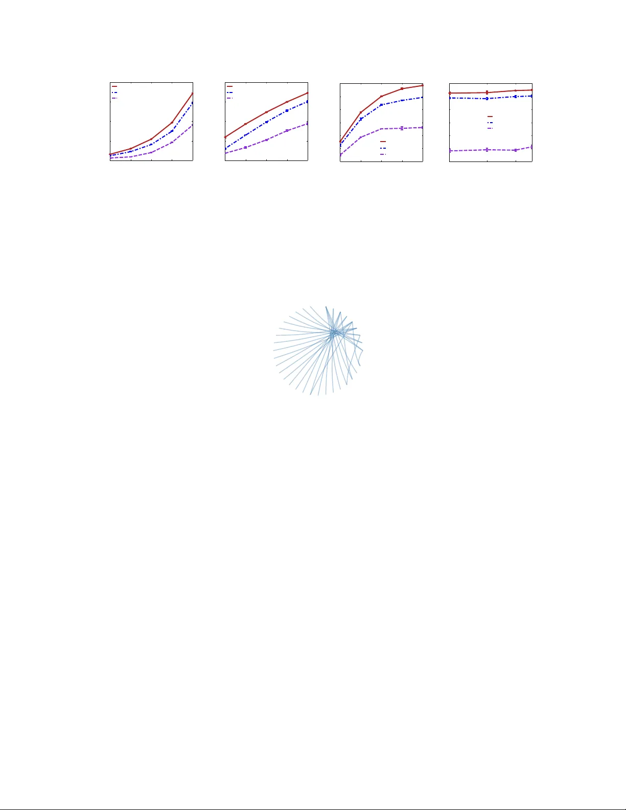
Comments & Academic Discussion
Loading comments...
Leave a Comment