The Need for Structure in Quantum Speedups

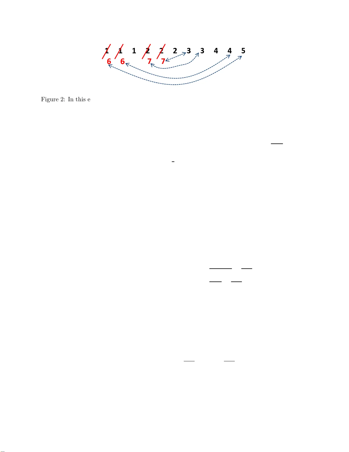
The Need for Structure in Quan tum Sp eedups Scott Aaronson ∗ MIT Andris Am bainis † Univ ersit y of Latvia and IAS, Princeton Abstract Is there a g eneral theorem that tells us when we can hop e for e x po nen tial sp eedups fr o m quantum algorithms, and when we canno t? In this pap er, we make tw o adv ances toward suc h a theor em, in the black-b ox model where mo st qua n tum alg orithms op erate. First, w e show that for an y proble m that is in v ariant under p ermuting inputs and outputs and that has suﬃciently man y outputs (like the collision and elemen t distinctness problems ), the quantum que r y complexit y is at lea s t the 7 th ro ot of the cla ssical ra ndomized que r y complexity . (An ear lier version o f this pap er gav e the 9 th ro ot.) This res olves a conjecture o f W atrous from 2002. Second, inspir ed by work o f O’Donnell et al. (20 05) and D inur et al. (2006), we conjecture that every bounded low-degree po lynomial has a “hig hly inﬂuential” v a riable. Assuming this conjecture, we show that every T -query qua n tum alg orithm can b e simulated o n most inputs by a T O (1) -query classica l algo rithm, and that one essentially cannot hop e to pr ove P 6 = BQP relative to a random o racle. 1 In tro duction P erhaps the cen tral lesson gleaned from ﬁfteen years of quantum algorithms r esearch is this: Quantum c omputers c an oﬀer sup erp olynom ial sp e e dups over classic al c omputers, b u t only for c ertain “structur e d” pr oblems . The k ey qu estion, of course, is wh at we mean b y “structured.” In the con text of most existing quan tum alg orithms, “structured ” basic ally means that we are trying to determine s ome global prop erty of an extremely long sequence of num b ers, assuming that the sequ en ce satisﬁes some global regularit y . As a canonical example, consider Period-Finding , the core of Shor’s algorithms for factoring and computing discr ete logarithms [29]. Here we are giv en b lac k-b o x access to an exp onent ially-long sequence of in tegers X = ( x 1 , . . . , x N ); that is, we can compute x i for a giv en i . W e are aske d to ﬁnd the p erio d of X —that is, th e smallest k > 0 such th at x i = x i − k for all i > k —promised that X is indeed p erio dic, w ith p erio d k ≪ N (and also that the x i v alues ∗ MIT. Email: aaronson@csail.mit.e du. This material is based up on w ork sup p orted by the National S cience F oundation und er Gran t No. 0844626, by a TIBCO Career Developmen t Chair, and by an Alan T. W aterman aw ard. † Email: ambai nis@lu.lv. Supp orted b y Universit y of Latv ia Research Grant ZP01-100, FP7 Marie Curie I nter- national R eintegration Grant (PIRG0 2-GA-2007-224886), FP7 FET-Op en pro ject QCS and ERC Adv anced Gran t MQC (at th e Universit y of Latvia) and the N ational Science F oun dation und er agreement No. DMS-1128155 (at IAS, Princeton). A ny opinions, ﬁ n dings and conclusions or recommendations exp ressed in th is material are those of the auth or(s) and do not necessarily reﬂ ect th e views of the National S cience F ound ation. 1 are approximat ely distinct within eac h p erio d). The r equ iremen t of p erio d icit y is crucial h ere: it is wh at lets us use the Quantum F ourier T ransform to extract the in f ormation we w an t from a sup erp osition of the form 1 √ N N X i =1 | i i | x i i . F or other kn o wn quan tum algorithms, X needs to b e (for example) a cyclic s hift of quadratic residues [16], or constan t on the cosets of a h idden sub group. By contrast, th e canonical example of an “unstr u ctured” problem is th e Gro v er searc h pr ob lem. Here w e are giv en b lack- b ox access to an N -bit string ( x 1 , . . . , x N ) ∈ { 0 , 1 } N , and are aske d whether there exists an i such that x i = 1. 1 Gro v er [20] ga v e a quan tum algorithm to solve th is problem using O ( √ N ) qu eries [20], as compared to th e Ω ( N ) needed classically . Ho w ev er, this quadratic sp eedu p is optimal, as shown by Benn ett, Berns tein, Brassard , and V azirani [10]. F or other “unstru ctured” prob lems—s uc h as computing the P arity or M ajority of an N -bit string— quan tum computers oﬀer n o asymptotic sp eedup at all o v er classical computers (see Beals et al. [8]). Unfortunately , this “need for structure” has essen tially limited the prosp ects for sup erp olyno- mial quan tum sp eedups to th ose areas of mathematics that are liable to pr o duce things like p erio dic sequences or sequences of quadratic residues. 2 This is the fundamental r e ason why the gr e atest suc c esses of qu antum algorithms r ese ar ch have b e en in crypto gr aphy, and sp e ciﬁc al ly in numb er- the or etic crypto gr aphy. It helps to explain why w e do not ha v e a fast quantum algorithm to solve NP -complete problems (for example), or to b reak arbitrary one-w a y fun ctions. Giv en th is h istory , the follo wing p roblem tak es on considerable imp ortance: Problem 1 (Informal) F or ev ery “u nstructur e d” pr oblem f , ar e the quantum q u ery c omplexity Q( f ) and the classic al r andomize d query c omplexity R( f ) p olynomial ly r elate d ? Despite its apparent v agueness, Pr oblem 1 can b e formalized in sev eral natural and convincing w a ys—and und er th ese formalizations, th e problem has r emained op en for ab out a decade. 1.1 F ormalizing the Problem Let S ⊆ [ M ] N b e a collectio n of in p uts, and let f : S → { 0 , 1 } b e a function that we are trying to compute. In this pap er , w e assume for simplicit y that th e range of f is { 0 , 1 } ; in other w ords, that w e are trying to solv e a d ecision problem. It will also b e con v enien t to think of f as a fu nction from [ M ] N to { 0 , 1 , ∗} , where ∗ means ‘und eﬁned’ (that is, th at a given inp ut X ∈ [ M ] N is not in f ’s domain S ). W e will w ork in the well- studied de cision-tr e e mo del . In this mo del, giv en an input X = ( x 1 , . . . , x N ), an algorithm can at any time choose an i and receiv e x i . W e count only the num b er of queries the algorithm mak es to the x i ’s, ignoring other computational steps. Then the deterministic query c omplexity of f , or D( f ), is the num b er of quer ies made by an optimal deterministic algorithm on a wo rst-case input X ∈ S . The (b ou n ded-error) r andomize d query c omplexity R( f ) is the 1 A va riant asks u s to ﬁnd an i such that x i = 1, under the mild promise that such an i exists. 2 Here we exclude BQ P -complete problems, such as simulating quantum physics (the “original” application of quantum computers), approximating the Jones p olynomial [4], and estimating a linear functional of the solution of a w ell-conditioned linear system [21]. 2 exp ected num b er of queries m ad e by an optimal rand omized algorithm that, f or ev ery X ∈ S , computes f ( X ) with probabilit y at least 2 / 3. The (b ou n ded-error) quantum query c omplexity Q( f ) is th e same as R( f ), except that we allo w quantum algorithms. Clearly Q( f ) ≤ R( f ) ≤ D( f ) ≤ N for all f . See Buhrman an d de W olf [15] for detailed deﬁnitions as well as a survey of these measures. If S = [ M ] N , then we sa y f is total , and if M = 2, th en we s a y f is Bo ole an . The case of total f is relativ ely well-understo o d. Already in 1998, Beals et al. [8] sh o w ed the follo wing: Theorem 2 (Beals et al.) D ( f ) = O (Q( f ) 6 ) for al l total Bo ole an functions f : { 0 , 1 } N → { 0 , 1 } . F urthermore, it is easy to generalize Th eorem 2 to sho w that D ( f ) = O (Q( f ) 6 ) for al l total functions f : [ M ] N → { 0 , 1 } , not necessarily Bo olean. 3 In other words, f or total fu nctions, th e quan tum query complexit y is alw a ys at least the 6 th ro ot of the classical query complexit y . The largest kno wn gap b et w een D( f ) and Q( f ) for a total fun ction is qu ad r atic, and is ac hiev ed by the OR fu nction (b ecause of Gr ov er’s algorithm). On the other hand, as so on as w e allo w non-total functions, w e can get enormous gaps. Aaron- son [2] ga v e a Bo olean fun ction f : S → { 0 , 1 } for wh ic h R( f ) = N Ω(1) , yet Q( f ) = O (1). 4 Other examples, for w hic h R( f ) = Ω( √ N ) and Q( f ) = O (log N log log N ), follo w easily from Simon’s al- gorithm [30] and Shor’s algorithm [29 ]. Intuitiv ely , these fu nctions f ac hiev e such large separations b y b eing highly s tr uctured: that is, their domain S includes only inpu ts that satisfy a strin gent promise, suc h as enco ding a p erio dic fun ction, or (in the case of [2]) enco ding t wo Bo olean functions, one of which is correlated with the F ourier transform of the other one. By contrast with these highly-stru ctured p r oblems, consider the c ol lision pr oblem : that of deciding whether a sequen ce of num b ers ( x 1 , . . . , x N ) ∈ [ M ] N is one-to-one (eac h num b er app ears once) or t w o-to-o ne (ea c h num b er app ears twice ). Let Col ( X ) = 0 if X is one-to-one and Col ( X ) = 1 if X is t w o-to-one, promised that one of these is the case. Then Col ( X ) is not a total function, since its deﬁn ition in v olv es a promise on X . In tuitiv ely , how ever, the collision problem seems muc h less “structured” than S imon’s and S hor’s pr oblems. One wa y to form alize this intuition is as follo ws. Call a p artial f unction f : [ M ] N → { 0 , 1 , ∗} p ermutation-invariant if f ( x 1 , . . . , x N ) = f ( τ ( x σ ( 1) ) , . . . , τ ( x σ ( N ) )) for all inputs X ∈ [ M ] N and all p ermutat ions σ ∈ S N and τ ∈ S M . Then Col ( X ) is p erm utation- in v ariant : we can p ermute a one-to-one sequ en ce and relab el its elements ho w ev er w e lik e, but it is s till a one-to-one sequence, and lik ewise for a tw o-to-one sequence. Because of this symmetry , attempts to solv e the collision p r oblem usin g (for example) th e Qu an tum F ourier T r ansform s eem unlik ely to succeed. And indeed, in 2002 Aaronson [1] pr o v ed that Q ( Col ) = Ω( N 1 / 5 ): that is, the quant um query complexit y of the collision pr oblem is at most p olynomially b etter than its r andomized query complexit y of Θ( √ N ). The qu an tum low er b ound w as later imp r o v ed to Ω( N 1 / 3 ) by Aaronson an d S h i [3], matc hing an u pp er b ound of Brassard , Høy er, and T app [13]. 3 Theorem 2 is proved by combining three ingredients: D( f ) = O (C( f ) bs( f )), C( f ) = O ( bs( f ) 2 ), and bs( f ) = O (Q( f ) 2 ) (where C( f ) is t h e c ertiﬁc ate c om plexity of f and bs( f ) is the blo ck sensitivity ). And all three ingredients go through with no essential change if w e set M > 2, and deﬁne suitable M -ary generalizations of C( f ) and bs( f ). (W e could also conv ert the non-Bo olean function f : [ M ] N → { 0 , 1 } to a Bo olean one, but then we w ould lose a factor of log M .) 4 Previously , de Beaudrap, Cleve , and W atrous [9] h ad stated a similar randomized versus q uantum separation. How ever, their separation applied not to th e standard q uantum black-b o x mo del, b u t to a diﬀerent mo del in which the blac k b ox p ermutes the answ er register | y i in some unkn o wn w ay (rather than simply mapping | y i to | y ⊕ f ( x ) i ). 3 Generalizing b oldly from this example, John W atrous (p ersonal communicatio n) conjectured that the randomized and quantum query complexities are p olynomially related f or every p ermutati on- in v ariant prob lem: Conjecture 3 (W atrous 2002) R( f ) ≤ Q( f ) O (1) for every p artial function f : [ M ] N → { 0 , 1 , ∗} that is p ermutation-invariant. Let us mak e t wo remarks ab out Conjecture 3. First, th e conjecture talks ab out r andomize d v ersus quantum query complexity , since in this setting, it is easy to ﬁnd functions f for w hic h R( f ) and Q( f ) are b oth tin y but D ( f ) is huge. As an example, consider the Deutsch-J ozsa pr oblem [17]: giv en a Bo olean input ( x 1 , . . . , x N ), decide whether the x i ’s are all equal or w hether half of them are 1 and the other half are 0, un der the p romise that one of these is the case. Second, if M = 2 (that is, f is Bo olean), then Conj ecture 3 follo ws relativ ely easily f rom kno wn results: indeed, w e pr ov e in App endix 6 that R( f ) = O (Q( f ) 2 ) in that case. So the interesti ng case is when M ≫ 2, as it is for the collision pr ob lem. Conjecture 3 provides one natural wa y to formalize the id ea that classical and quantum query complexities should b e p olynomially related for all “unstru ctured” problems. A diﬀeren t wa y is pro vided b y th e follo wing conjecture, wh ic h we we re a w are of since ab out 1999: Conjecture 4 (folklore) L et Q b e a quantum algorithm that makes T queries to a Bo ole an input X = ( x 1 , . . . , x N ) , and let ε > 0 . Then ther e exists a deterministic classic al algorith m that makes p oly( T , 1 /ε, 1 /δ ) que rie s to the x i ’s, and that appr oximates Q ’s ac c eptanc e pr ob ability to within an additive err or ε on a 1 − δ fr action of inputs. But w hat exactly d o es Conjecture 4 ha v e to do with “the need for structure in q u an tum sp eedup s”? With Conjecture 3, the connection to this p ap er’s th eme w as more-or-less obvious, but w ith Conjecture 4, s ome additional explanation is probably needed. In tuitiv ely , we w an t to sa y th e follo wing: in ord er to ac hiev e a sup erp olynomial sp eedup in the blac k-b o x mo del, a quantum computer needs not merely a promise problem, bu t a “sev erely constrained” p romise prob lem. In other w ords, only a minuscule fr action of th e 2 N oracle str in gs X = ( x 1 , . . . , x N ) ough t to satisfy the pr omise—precisely lik e w h at happ ens in Simon ’s and Shor’s problems, w h ere the promise asserts that X enco des a p erio dic fun ction. I f the pr omise is to o “mild”—if, say , it h olds for all X in some set S ⊆ { 0 , 1 } N with | S | = Ω(2 N )—then we should b e bac k in the situation studied by Beals et al. [8], where the oracle X lac ked enough “structure” for a Shor-like algorithm to exploit, and as a resu lt, the b est one could h op e for w as a p olynomial quan tum sp eedup like that of Gro v er’s algorithm. Y et, if w e interpret the ab ov e intuitio n to o na ¨ ıv ely , th en it is easy to ﬁnd counterexamples. T o illustrate, let S 1 consist of all strings X ∈ { 0 , 1 } N that enco de v alid inp uts to Simon’s problem, let S 0 consist of all Y ∈ { 0 , 1 } N that hav e Hamming d istance at least N / 10 from ev ery X ∈ S 1 , and let S = S 0 ∪ S 1 . Th en deﬁne a Bo olean fun ction f Simon : S → { 0 , 1 } b y f Simon ( X ) = 1 for all X ∈ S 1 , and f Simon ( X ) = 0 for all X ∈ S 0 . As observ ed by Buh rman et al. [14] (see also Am bainis and de W olf [6] and Hemaspaand r a, Hemaspaandra, and Zimand [22]), this “p r op ert y- testing v ersion of Simon’s problem” ac h iev es an exp onen tial s ep aration b et w een randomized and quan tum query complexities: R( f Simon ) = Ω( p N/ log N ) wh ile Q( f Simon ) = O (log N ). But the promise is certainly “mild”: indeed | S | ≥ 2 N − 2 cN for some constan t c < 1. On th e other h an d , examining th is counterexample more closely su ggests a wa y to salv age our original int uition. F or notice that there exists a fast, deterministic classical algorithm that correctly 4 ev aluates f Simon ( X ) on almost al l inputs X ∈ S : n amely , the algorithm that alwa ys outputs 0! T h is algorithm errs only on the m in uscule fraction of inputs X ∈ S that happ en to b elong to S 1 . Thus, w e might conjecture that this p oints to a general ph enomenon: namely , wheneve r there exists a fast quan tum algorithm to compu te a Bo olean function f : S → { 0 , 1 } w ith | S | = Ω  2 N  , there also exists a fast classical algorithm to compu te f ( X ) on most inp u ts X ∈ S . In App endix 8, we will p ro v e th at Conjecture 4 is equiv alen t to th is conjecture. Indeed, Conjecture 4 readily implies a far-reac hing generalization of the result of Beals et al. [8] stating that D( f ) = O (Q( f ) 6 ) for all total Bo olean fun ctions f . In particular, deﬁn e the ε -appr oximate query c omplexity of a Bo olean fu n ction f : { 0 , 1 } N → { 0 , 1 } , or D ε ( f ), to b e the minim um num b er of queries made by a deterministic algorithm that ev aluates f correctly on at least a 1 − ε fraction of inputs X . Lik ewise, let Q ε ( f ) b e the minimum num b er of queries made b y a quan tum algorithm that ev aluates f correctly on at least a 1 − ε fraction of inputs. Then Conjecture 4 implies that D ε ( f ) and Q δ ( f ) are p olynomially related for all Bo olean fun ctions f and all constan ts ε > δ > 0 indep end en t of N . 5 This wo uld provide a qu an tum coun terpart to a b eautiful 2002 result of S m yth [31], who solv ed an old op en problem of Stev en Rudic h b y s h o wing that D ε ( f ) = O (C ε 3 / 30 ( f ) 2 /ε 3 ) for all ε > 0 (where C δ ( f ) denotes th e “ δ -appro ximate certiﬁcate complexit y” of f ). More dramatically , if C onjecture 4 holds, then we b asic al ly c annot hop e to pr ove P 6 = BQP r elative to a r andom or acle. This w ould answer a question raised by F ortno w and R ogers [19] in 1998, and w ould cont rast sh arply with the situation for non -rand om oracles: we h av e had oracles relativ e to whic h P 6 = BQP , and indeed B QP 6⊂ M A , since the w ork of Bernstein and V azirani [11] in the early 1990s. More precisely , und er some su itable complexity assumption (suc h as P = P # P ), w e would get BQP A ⊂ AvgP A with pr obabilit y 1 for a rand om oracle A . Here AvgP is the class of languages for w hic h there exists a p olynomial-time algorithm that solves a 1 − o (1) fraction of instances of size n . In other words, s ep arating B QP from AvgP r elativ e to a r an d om oracle w ould b e as hard as separating complexit y classes in the u nrelativized world. This would provide a quant um coun terpart to a theorem of Impagliazzo and Ru dic h (credited in [23]), who used th e p o w erful results of Kahn, S aks, and Smyth [23] to show that if P = NP , then NP A ∩ coNP A ⊂ ioAvgP A with probabilit y 1 for a random oracle A . 6 1.2 Our R esults Our main contribution in this pap er is essen tially to prov e W atrous’s conjecture (Conjecture 3), that randomized an d quant um qu er y complexities are p olynomially related for every symmetric problem. Theorem 5 R( f ) = O (Q ( f ) 7 p olylog Q( f )) for every p artial function f : [ M ] N → { 0 , 1 , ∗} that is p ermutation-invariant. W e conjecture that R( f ) and Q( f ) are p olynomially r elated ev en for f unctions f satisfying one of the tw o symmetries: namely , f ( x 1 , . . . , x N ) = f ( x σ ( 1) , . . . , x σ ( N ) ) for all σ ∈ S N . W e also conjecture that th e exp onen t of 7 can b e impro v ed to 2: in other w ords, that Gr ov er’s algorithm once again provides the optimal sep aration b et ween the quan tum and classical mo dels. 5 More generally , as w e will show in Corollary 23, the relation we obtain is D ε + δ ( f ) ≤ ( Q ε ( f ) /δ ) O (1) for all ε , δ > 0. 6 Here ioAvgP means “av erage-case P for inﬁnitely many input lengths n .” The reason Impagliazzo and Rudich only get a simulation in ioAvgP , rather th an AvgP , has to do with the fact that Smyth’s result [31 ] only relates D ε ( f ) to C ε 3 / 30 ( f ), rather th an D ε + δ ( f ) t o C ε ( f ) for all δ > 0. 5 While the pr o of of Theorem 5 is somewh at in v olv ed, it can b e entirely u ndersto o d by those unfamiliar with quantum computing: th e d iﬃ cu lties lie in getting the pr oblem into a form wh er e existing quantum lo w er b ound tec hn ology can b e applied to it. Let u s stress that it was n ot at all ob vious a priori that existing quant um lo we r b oun ds w ould suﬃ ce here; that they did came as a surpr ise to us. W e ﬁ rst d eﬁne and analyze a simp le randomized algorithm, whic h tries to compute f ( X ) for a giv en X = ( x 1 , . . . , x N ) b y estimating the multiplicit y of eac h elemen t x i . Next, by considering where this randomized algorithm b reaks do wn, we sh o w that one can identi fy a “hard core” within f : roughly sp eaking, t wo input t yp es A ∗ and B ∗ , suc h that the diﬃ cu lt y of distinguish ing A ∗ from B ∗ accoun ts for a p olynomial fraction of the entire diﬃcult y of computing f . The rest of the pro of consists of lo w er-b ound ing the quantum query complexit y of distinguishing A ∗ from B ∗ . W e do so using a hybrid argumen t: w e d ev elop a “c hopping pro cedu re” that gradually deforms A ∗ to make it more similar to B ∗ , creating a sequence of in termediate inpu t types A 0 = A ∗ , A 1 , A 2 , . . . , A 2 L = B ∗ . W e then sh ow th at, for ev ery ℓ ∈ [ L ] , d istinguishing A ℓ from A ℓ − 1 requires many quantum queries, either by a reduction from Zhandr y’s recen t Ω( N 1 / 3 ) quan tum lo w er b ound for the Set Equality problem [33] (wh ic h is a n on trivial generalization of Aaronson and S h i’s collision lo w er b oun d [3]), or else by an application of Am bainis’s general q u an tum adversary theorem [5]. Note that, prior to Zhandr y’s Ω( N 1 / 3 ) qu an tum lo w er b ound for Set Equality , Midrijanis [24] h ad p ro v ed a low er b ound of Ω(( N / log N ) 1 / 5 ); the latter wa s the ﬁrst quant um low er b ound for SetEqual ity , and the only one for n early a decade. An earlier version of this p ap er used Midrijanis’s lo w er b ound to show that R( f ) = O (Q( f ) 9 p olylog Q( f )) for all p ermutation-symmetric f . The impr o v emen t to R( f ) = O (Q( f ) 7 p olylog Q( f )) in the current v ersion comes en tirely from Zhandr y ’s impro v emen t of the Se tEquality lo w er b oun d to the optimal Ω( N 1 / 3 ). Doing the hybrid argument in the “obvio us” w a y pro duces a b oun d of the form R( f ) ≤ Q( f ) O (1) p olylog N , whic h fails to imply a p olynomial relationship b et w een R( f ) and Q( f ) when Q( f ) ≤ (log N ) o (1) . Ho w ev er, a more sop h isticated hybrid argumen t eliminates the p olylog N factor. Our second con tribution is more exploratory , something we p ut forward in the hop e of inspir in g follo w up work. W e study Conjecture 4 , which states that ev ery T -query quantum algo rithm can b e sim ulated on most inpu ts u sing T O (1) classical queries. W e relate th is conjecture to a fun damen tal op en p roblem in F ourier analysis and appro ximation theory . Give n a real p olynomial p : R N → R , let Inf i [ p ] := E X ∈{ 0 , 1 } N  ( p ( X ) − p ( X i )) 2  b e the inﬂuenc e of the i th v ariable, where X i means X with the i th bit ﬂipp ed. T h en we conjecture that eve ry b ounde d low-de gr e e p olynomial has a “highly inﬂuential” v ariable . More precisely: Conjecture 6 (Bounded P olynomials Ha v e Inﬂuen tial V ariables) L et p : R N → R b e a p olynomial of de gr e e d . Supp ose that 0 ≤ p ( X ) ≤ 1 for al l X ∈ { 0 , 1 } N , and E X ∈{ 0 , 1 } N  ( p ( X ) − E [ p ]) 2  ≥ ε. Then ther e exists an i such that I nf i [ p ] ≥ ( ε/d ) O (1) . W e show the follo wing: 6 Theorem 7 Assume Conje ctur e 6. Then (i) Conje ctur e 4 holds. (ii) D ε + δ ( f ) ≤ ( Q ε ( f ) /δ ) O (1) for al l Bo ole an functions f : { 0 , 1 } N → { 0 , 1 } and al l ε, δ > 0 . (iii) If P = P # P , then BQP A ⊂ AvgP A with pr ob ability 1 for a r andom or acle A . The main evidence f or Conjecture 6—b esides the fact that all the F our ier analysis exp erts w e ask ed were conﬁdent of it!—is that extremely similar statemen ts ha v e recen tly b een p ro v ed. Firstly , O’Donnell, Saks, Sc hramm, and Servedio [26] prov ed an analogue of Conjecture 6 for de cision tr e es , whic h are a sp ecial case of b ounded real p olynomials: Theorem 8 (O’Donnell et al. 2005) L et f : { 0 , 1 } N → { 0 , 1 } b e a Bo ole an f u nction, and sup- p ose Pr [ f = 1] Pr [ f = 0] ≥ ε . Then ther e exists an i such that Inf i [ f ] ≥ 4 ε/ D ( f ) , wher e D ( f ) is the de cision tr e e c omplexity of f . Unfortunately , Th eorem 8 do es not d irectly imply anything ab out our problem, ev en though Beals et al. [8] sh o w ed th at D ( f ) and Q( f ) are p olynomially related for all total Bo olean f u nctions f . The r eason is th at the acceptance p r obabilit y of a quant um algorithm need not appro ximate a total Bo olean fu nction. The second piece of evidence for Conjecture 6 comes from a p o w erful result of Din ur, F riedgut, Kindler, and O’Donnell [18 ], whic h imp lies our conjecture, exc ept with In f i [ p ] ≥ ε 3 / 2 O ( d ) instead of I n f i [ p ] ≥ ( ε/d ) O (1) . Let us s tate the sp ecial case of their result that is relev ant f or us: Theorem 9 (Dinur e t al. 2006) L et ε > 0 , and let p : R N → R b e a de gr e e- d p olynomial su c h that 0 ≤ p ( X ) ≤ 1 for al l X ∈ { 0 , 1 } N . Then ther e exists a 2 O ( d ) /ε 2 -junta e p : R N → R (that is, a p olynomial dep ending on at most 2 O ( d ) /ε 2 variables) such that E X ∈{ 0 , 1 } N h ( e p ( X ) − p ( X )) 2 i ≤ ε. Ev en though Th eorem 9 h as an exp onentia l rather than p olynomial dep enden ce on 1 /d , w e observ e that it alr e ady has a non trivial consequence f or quantum computation. Namely , it implies that an y T -query quantum algorithm can b e simulated on most in p uts us ing 2 O ( T ) classical queries. 7 Recall that the gaps b et ween classical and quantum query complexities can b e sup erexp onen tial (and ev en N Ω(1) v ersus O (1), as in the example of Aaronson [2]), so eve n an exp onen tial upp er b ound is far from ob vious. 1.3 Subsequen t W ork Since the ﬁrst ve rsion of this pap er wa s circulated, there h a v e b een at least three interesti ng dev elopmen ts (not counting the Ω( N 1 / 3 ) qu an tum lo we r b ound of Zhandr y [33] for Set Equality , whic h we incorp orate here). First, Y uen [32] adapted th e hybrid argument that we used to pr ov e Theorem 5, in order to sho w that distinguish ing a random fun ction X : [ N ] → [ N ] fr om a random p erm utation requir es 7 Indeed, in t h is case the classical queries are nonadaptive. 7 Ω( N 1 / 5 / log N ) quan tum queries. (Subsequ en tly , ho w ev er, Z handry [33] p ro v ed a tight lo w er b ound of Ω( N 1 / 3 ) for the rand om fu nction versus random p erm utation problem, using completely diﬀeren t ideas.) Second, Mont anaro [25] u sed a hypercontract iv e in equalit y to prov e Conjecture 6, in the sp ecial case where p is a multili near p olynomial all of w hose co eﬃcien ts (when wr itten in the F ourier basis) ha v e the same absolute v alue. Cur ren tly , it r emains op en to generalize Mon tanaro’s tec hniqu e to arbitrary multilinear p olynomials, let alone arbitrary p olynomials. Third, Ba ˇ ckurs and Ba v arian [7] solv ed a tec hnical pr ob lem that arose from an earlier v ersion of this p ap er. In th e earlier version, we stated Conjecture 6 in term s of L 1 -inﬂuences rather than L 2 -inﬂuences, and we also u sed the L 1 -norm in proving the consequen ces of Conjecture 6 for quan tum query complexit y . Subsequently , Ba ˇ ckurs (p ersonal comm unication) found an err or in our pro of. F ortunately , h o w ev er, we noticed that (a) our pro of could b e ﬁxed b y simply switc hing from L 1 -norm to L 2 -norm throughout, and (b) the L 2 v ersion of Conjecture 6 w as, in any case, pro v ably equiv alen t to our original L 1 v ersion. So we sw itc h ed to the L 2 -norm. At the same time, though, w e r emained curious ab out our original L 1 -based argu m en t c ould have work ed. The question b oiled d o wn to the follo wing: giv en a degree- d real p olynomial p : R N → R , let Inf 1 i [ p ] := E X ∈{ 0 , 1 } N    p ( X ) − p ( X i )    . Then do w e hav e P N i =1 Inf 1 i [ p ] ≤ d O (1) , w henev er p ( X ) ∈ [0 , 1] f or all X ∈ { 0 , 1 } N ? Ba ˇ ckurs and Ba v arian [7] sho w that the answ er is y es: indeed, the su m of the L 1 -inﬂuences is upp er-b ound ed b y O ( d 3 log d ). Usin g their result, one c an salv age our original L 1 -based argument. F or simp licit y , though, in this version of the p ap er we s tic k with L 2 -inﬂuences. There, the analogue of Ba ˇ ckurs and Ba v arian’s result is muc h easier, an d states that P N i =1 Inf i [ p ] ≤ d (we pro vide the folklore pro of in Lemma 20). F or completeness, in App endix 7 we prov e the equiv alence of th e L 1 and L 2 v ersions of Conj ecture 6. 2 Quan tum Lo w er Bound for All Symmetric Problems In this section w e pro v e Theorem 5: that R( f ) = O (Q( f ) 7 p olylog Q( f )) for all p ermutation- symmetric f . W e start w ith a s im p le observ ation that is essen tial to ev erything that follo ws. Since f is symmetric, we can group the inp uts X = ( x 1 , . . . , x N ) into equiv alence classes that w e call typ es . Deﬁnition 10 Given an input X = ( x 1 , . . . , x N ) ∈ [ M ] N , the typ e of X is a list of p ositive inte gers A = ( a 1 , . . . , a u ) , which r e c or ds the multiplicities of the inte gers o c curring in X fr om most to le ast fr e qu ent. So in p articular, a 1 ≥ · · · ≥ a u and a 1 + · · · + a u = N . F or c onvenienc e, we adopt the c onvention that a i = 0 for al l i > u . In other w ords, a t yp e is just a partition (or Y oung diagr am ) that records th e multipliciti es of the inp ut element s. F or example, a one-to-one inp u t h as t yp e a 1 = · · · = a N = 1, while a t w o-to-o ne inpu t has t yp e a 1 = · · · = a N/ 2 = 2. W e wr ite X ∈ A if X is of t yp e A . Clearly f ( X ) dep ends only on the t yp e of X . F urthermore, giv en a quant um qu ery algorithm Q , w e can assume without loss of generalit y th at Pr [ Q accepts X ] dep end s only on the type of X —sin ce w e can “symm etrize” Q (that is, r andomly p erm ute X ’s in puts an d outputs) pr ior to ru nning Q . 8 2.1 Randomized Upp er Bound Let X = ( x 1 , . . . , x N ) b e an inpu t. F or eac h j ∈ [ M ], let κ j b e the n umber of i ’s such that x i = j . Then the ﬁrst step is to give a classical rand omized algorithm th at estimates the κ j ’s. This algorithm, S T , is an extremely straight forward sampling p ro cedure. (Ind eed, there is essentia lly nothing else that a rand omized algorithm can do h ere.) S T will make O ( T 1+ c log T ) qu eries, wh ere T is a parameter and c ∈ (0 , 1] is a constan t that we will c ho ose later to optimize the ﬁnal b ound . Set U := 21 T 1+ c ln T Choose U indices i 1 , . . . , i U ∈ [ N ] unifo rmly at random with replacement Query x i 1 , . . . , x i U For each j ∈ [ M ] : Let z j be the number of occurr ences of j in ( x i 1 , . . . , x i U ) Output e κ j := z j U · N as the estimate for κ j W e now analyze how w ell S T w orks. Lemma 11 W ith pr ob ability 1 − O (1 /T ) , we have | e κ j − κ j | ≤ N T + κ j T c for al l j ∈ [ M ] . Pro of. F or eac h j ∈ [ M ], we consider four cases. Firs t supp ose κ j ≥ N/T 1 − c . Notice that z j is a su m of U indep end en t Boolean v ariables, and that E [ z j ] = U N E[ e κ j ] = U N κ j . Thus Pr h | e κ j − κ j | > κ j T c i = Pr      z j − U N κ j     > U κ j N T c  < 2 exp  − U κ j / N 3 T 2 c  < 2 exp  − U 3 T 1+ c  = 2 T − 7 , where the second line follo ws from a Ch ernoﬀ b ound and the third from κ j ≥ N /T 1 − c . Second, su p p ose N /T ≤ κ j < N /T 1 − c . Then Pr  | e κ j − κ j | > N T  = Pr      z j − U N κ j     > U T  < 2 exp − U κ j / N 3  N T κ j  2 ! < 2 exp  − U 3 T 1+ c  = 2 T − 7 where the second line follo ws fr om a Chernoﬀ b ound (which is v alid b ecause N T κ j ≤ 1) and the third from κ j < N /T 1 − c . 9 Third, su pp ose N /T 6 ≤ κ j < N /T . Then Pr  | e κ j − κ j | > N T  = Pr      z j − U N κ j     > U T  < e N/ ( T κ j ) (1 + N / ( T κ j )) 1+ N/ ( T κ j ) ! U κ j / N ≤ exp  − N T κ j · U κ j N  = exp  − U T  = O  1 T 7  , where the second line follo ws from a Cher n oﬀ b oun d, the third line follo ws from N T κ j > 1, and the last follo ws f rom U = 21 T 1+ c ln T . F ourth, sup p ose κ j < N /T 6 . Then Pr  | e κ j − κ j | > N T  = Pr      z j − U N κ j     > U T  ≤ Pr [ z j ≥ 2] ≤  U 2   κ j N  2 ≤ U 2 T 6  κ j N  ≤ κ j T N for all su ﬃcien tly large T , where the second line follo w s from κ j < N /T 6 , the third f rom th e union b ound , the fourth from κ j < N /T 6 (again), and the ﬁfth from U ≤ 21 T 2 ln T . Notice that th ere are at most T 6 v alues of j suc h that κ j ≥ N/T 6 . Hence, pu tting all four cases together, Pr  ∃ j : | e κ j − κ j | > N T + κ j T c  ≤ T 6 · O  1 T 7  + X j : κ j 2 N T + a i + b i T c . Then R T c omputes f with b ounde d pr ob ability of e rr or, and henc e R ( f ) = O ( T 1+ c log T ) . Pro of. First supp ose X ∈ A where A = ( a 1 , a 2 , . . . ) is a 1-t yp e. T hen b y Lemma 11, with probabilit y 1 − O (1 /T ) w e ha v e | e κ i − a i | ≤ N T + a i T c for all i . (It is easy to see th at sorting the e κ i ’s can only decrease th e maxim um diﬀerence.) Pro vided this o ccurs, R T ﬁnds some 1-t yp e close to ( e κ 1 , e κ 2 , . . . ) (p ossibly A itself ) and outp u ts f ( X ) = 1. Second, supp ose X ∈ B where B = ( b 1 , b 2 , . . . ) is a 0-type. Then with p r obabilit y 1 − O (1 /T ) w e hav e | e κ i − b i | ≤ N T + b i T c for all i . Pro vided this o ccurs, by the triangle inequalit y , for ev ery 1-t yp e A = ( a 1 , a 2 , . . . ) there exists an i such that | e κ i − a i | ≥ | a i − b i | − | e κ i − b i | > N T + a i T c . Hence R T do es not ﬁ nd a 1-t yp e close to ( e κ 1 , e κ 2 , . . . ), and it outputs f ( X ) = 0. In p articular, supp ose w e k eep decreasing T until there exists a 1-t yp e A ∗ = ( a 1 , a 2 , . . . ) and a 0-t yp e B ∗ = ( b 1 , b 2 , . . . ) su ch that | a i − b i | ≤ 2 N T + a i + b i T c (1) for all i , s topp ing as so on as that happ ens. Then Lemma 12 implies that we will still ha v e R ( f ) = O ( T 1+ c log T ). F or the rest of the pro of, w e will ﬁx that “almost as small as p ossible” v alue of T for which (1) holds, as well as the 1-t y p e A ∗ and the 0-t yp e B ∗ that R T “just barely distinguishes” fr om one another. 2.2 The Chopping P ro cedure Giv en t w o sets of inputs A and B with A ∩ B = ∅ , let Q( A, B ) b e the minimum num b er of quer ies made by an y quantum algorithm that accepts ev ery X ∈ A with probabilit y at least 2 / 3, and accepts ev ery Y ∈ B with pr obabilit y at most 1 / 3. Also, let Q ε ( A, B ) b e the minimum num b er of queries made by an y quantum algorithm th at accepts ev ery X ∈ A with at least some probab ility p , and that accepts eve ry Y ∈ B with probability at most p − ε . Then we h a v e th e follo win g basic relation: Prop osition 13 Q( A, B ) = O ( 1 ε Q ε ( A, B )) for al l A, B and al l ε > 0 . Pro of. This f ollo ws from standard amplitude estimation tec hniqu es (see Brassard et al. [12] for example). The rest of the p ro of consists of low er-b ounding Q( A ∗ , B ∗ ), the quantum qu er y complexity of distinguishing inputs of t yp e A ∗ from inputs of t yp e B ∗ . W e do this via a hybrid argument. Let L := ⌈ log 2 N ⌉ + 1. A t a high lev el, we will constru ct a sequence of t yp es A 0 , . . . , A 2 L suc h th at 11 (i) A 0 = A ∗ , (ii) A 2 L = B ∗ , and (iii) Q( A ℓ , A ℓ − 1 ) is large for ev ery ℓ ∈ [2 L ]. Pro vided we can do this, it is not hard to see that we get the desir ed lo w er b ound on Q( A ∗ , B ∗ ). Supp ose a quantum algorithm distinguishes A 0 = A ∗ from A 2 L = B ∗ with constant b ias. Th en b y the triangle inequalit y , it must also d istinguish some A ℓ from A ℓ +1 with reasonably large bias (sa y Ω (1 / log N )). By Prop osition 13, an y qu an tum algorithm that succeeds with bias ε can b e ampliﬁed, with O (1 /ε ) o v erhead, to an algorithm that succeeds with constant bias. Inciden tally , the need, in this hybrid argument, to amplify the distinguish ing bias ε = ε ℓ from Ω (1 / log N ) to Ω (1) is exactly what could pr o duce an u ndesired 1 / log N factor in our ﬁnal lo w er b ound on Q( f ), if w e were n ot careful. (W e mentio ned this issue in Section 1.2.) T h e wa y we will solv e this problem, rou gh ly sp eaking, is to design the A ℓ ’s in such a wa y that our lo w er b ounds on Q( A ℓ , A ℓ − 1 ) increase quic kly as fu nctions of ℓ . That wa y , we can tak e the biases ε ℓ to decrease quadratically with ℓ (thus su mming to a constan t), y et still h a v e Q( A ℓ , A ℓ − 1 ) increasing quic kly enough that Q ε ℓ ( A ℓ , A ℓ − 1 ) = Ω( ε ℓ Q( A ℓ , A ℓ − 1 )) remain “unif orm ly large,” with 1 / log T factors but no 1 / log N factor. W e now describ e the pro cedure for creating the in termediate types A ℓ . In tuitiv ely , we w ant to form A ℓ from A ℓ − 1 b y making its Y oun g diagram more similar to that of B ∗ , by decreasing the ro ws of A ℓ − 1 whic h are larger than the corresp onding rows of B ∗ and increasing the rows of A ℓ − 1 whic h are sm aller than the corresp onding r o ws of B ∗ . More precisely , we construct the in termediate t y p es A 1 , A 2 , . . . v ia the follo wing pro cedure. In this pr o cedure, ( a 1 , a 2 , . . . ) is an input t yp e that is in itialize d to A ∗ , and B ∗ = ( b 1 , b 2 , . . . ). let P be the first power of 2 greater than or equal to N for ℓ := 1 to L let S A be the set of i such that a i − b i ≥ P / 2 l let S B be the set of i such that b i − a i ≥ P / 2 l let m := min( | S A | , | S B | ) choose m e lements i from S A , set a i := a i − P / 2 ℓ and remove them from S A choose m e lements i from S B , set a i := a i + P / 2 ℓ and remove them from S B let A 2 ℓ − 1 := t yp e( a 1 , a 2 , . . . ) if | S A | > 0 let a i := a i − P / 2 ℓ for all i ∈ S A choose | S A | elements i such that a i < b i and set a i := a i + P / 2 ℓ if | S B | > 0 let a i := a i + P / 2 ℓ for all i ∈ S B choose | S B | elements i such that a i > b i and set a i := a i − P / 2 ℓ let A 2 ℓ := t yp e( a 1 , a 2 , . . . ) next ℓ The p ro cedure is illustrated pictorially in Figure 1. 12 Figure 1: C hopping a ro w of A ℓ ’s Y oung diagram to make it more similar to B ℓ . W e start w ith some s imple obs er v ations. First, by construction, this pro cedure halts after 2 L = O (log N ) iterations. Second, after the ℓ th iteration, w e h av e | a i − b i | < P 2 ℓ for all i . This follo w s by induction. L et a ′ i b e the v alue of a i b efore the ℓ th iteration. Because of the in ductiv e assumption, we must ha v e | a ′ i − b i | < P 2 ℓ − 1 —for if | a ′ i − b i | ≥ P 2 ℓ , then a i is c hanged b y P 2 ℓ during the ℓ th iteration, to decrease the diﬀerence | a i − b i | . After this change, | a i − b i | =   a ′ i − b i   − P 2 ℓ < P 2 ℓ − 1 − P 2 ℓ = P 2 ℓ . Besides the | a ′ i − b i | ≥ P 2 ℓ case, there is one other case where | a i − b i | could c h ange. In the transition from A 2 ℓ − 1 to A 2 ℓ , if | S A | > 0 or | S B | > 0, then we c h ange a i for | S A | or | S B | elements i th at do not b elong to S A or S B . F or those elemen ts, w e ha v e | a i − b i | < P 2 ℓ and we c hange a i in the direction of b i (w e increase it b y P 2 ℓ if a i < b i and decrease it b y the same amount if a i > b i ). Therefore, after the c hange, the sign of th e diﬀerence a i − b i ﬂips and | a i − b i | < P 2 ℓ . No w let u s deﬁne kA − B k := 1 2 N X i =1 | a i − b i | . Notice that kA ℓ − A ℓ − 1 k = r P / 2 ℓ ′ , where r is the n umber of rows that get increased (or decreased) in the ℓ th iteration and l ′ = ⌈ l 2 ⌉ . W e now pro v e an upp er b ound on kA ℓ − A ℓ − 1 k wh en ℓ is sm all, whic h w ill b e useful later. Lemma 14 If ℓ ≤ ( log 2 T ) − 2 , then kA 2 ℓ − 2 − A 2 ℓ − 1 k + k A 2 ℓ − 1 − A 2 ℓ k ≤ 4 N T c . Pro of. Let m := max( | S A | , | S B | ). Then kA 2 ℓ − 2 − A 2 ℓ − 1 k + k A 2 ℓ − 1 − A 2 ℓ k = m P 2 ℓ . Without loss of generalit y , we assume th at m = | S A | . T o show the lemma, it suﬃces to pro ve that | S A | ≤ 4 N/T c P / 2 ℓ . W e consider the sum P j ∈ R | a j − b j | wh ere R is the set of all j suc h that | a j − b j | ≥ P 2 ℓ , with ( a 1 , a 2 , . . . ) ev olving from A 0 to A 2 ℓ − 2 and B ∗ = ( b 1 , b 2 , . . . ) ﬁxed. I n itially (when ( a 1 , a 2 , . . . ) = A 0 ), we hav e P 2 ℓ ≤ | a j − b j | ≤ 2 N T + a j + b j T c 13 for eac h j ∈ R . Since ℓ ≤ (log 2 T ) − 2, the left in equalit y implies | a j − b j | ≥ 4 N T , whic h combined w ith the righ t inequalit y yields a j + b j T c ≥ 2 N T . (2) Therefore X i ∈ R | a i − b i | ≤ X i ∈ R  2 N T + a i + b i T c  ≤ 2 X i ∈ R a i + b i T c ≤ 4 N T c , where the third line uses (2). The su m P i ∈ R | a i − b i | is not increased by an y step of the algorithm that generates A 0 , . . . , A 2 ℓ − 2 . Therefore, at the b eginning of the ℓ th iteration, we still ha v e P i ∈ R | a i − b i | ≤ 4 N T c . This means that | S A | ≤ 4 N/T c P / 2 ℓ . 2.3 Quan t um Lo w er Bounds Recall that we listed four pr op erties th at we needed the chopping pro cedure to satisfy . W e hav e already seen that it satisﬁes pr op erties (i)-(ii), so the remainin g step is to sh o w that it satisﬁes prop erty (iii). T hat is, w e need to lo w er-b oun d Q( A ℓ , A ℓ − 1 ), the b ounded-error quantum qu ery complexit y of d istinguishing inpu ts of t yp e A ℓ from inputs of t yp e A ℓ − 1 . T o d o this, it will b e con v enien t to consid er tw o cases: ﬁrst, that forming A ℓ in v olv ed c hopping few elemen ts of A ℓ − 1 , and second, th at it inv olv ed c hopping many elements. W e will show that w e “win either wa y ,” by a d iﬀeren t qu an tum lo w er b ound in eac h case. First consider the case that few elemen ts w ere chopp ed. Here we p ro v e a lo w er b ound using Am bainis’s quantum adve rsary metho d [5], in its “general” form (the one used, for example, to lo w er-b ound the quantum query complexit y of inv erting a p ermutati on). F or completeness, w e no w state Ambainis’s adversary theorem in the form we will need. Theorem 15 (Am bainis [5]) L et A, B ⊆ [ M ] N b e two sets of inputs with A ∩ B = ∅ . L et R ⊆ A × B b e a r elation on input p airs, suc h that for every X ∈ A ther e exists at le ast one Y ∈ B with ( X, Y ) ∈ R and vic e v e rsa. Given inputs X = ( x 1 , . . . , x N ) in A and Y = ( y 1 , . . . , y N ) in B , let q X,i = Pr Y ∈ B [ x i 6 = y i | ( X, Y ) ∈ R ] , q Y , i = P r X ∈ A [ x i 6 = y i | ( X, Y ) ∈ R ] . Supp ose that q X,i q y , i ≤ α for ev ery ( X , Y ) ∈ R and every i ∈ [ N ] such that x i 6 = y i . Then Q( A, B ) = Ω (1 / √ α ) . 14                Figure 2: In this example, N = 11, r = 2, P / 2 ℓ = 2, and a 1 = a 2 = 3. So w e transform X to Y by c ho osing h 1 = 1 and h 2 = 2, c hanging any t w o element s equ al to h 1 and an y t w o elemen ts equal to h 2 , and then sw apping the four elemen ts that we c hanged with fou r un c hanged elemen ts. Using T heorem 15, w e can p ro v e th e follo wing lo w er b ound on Q ( A ℓ , A ℓ − 1 ). Lemma 16 L et d = k A ℓ − A ℓ − 1 k , and assume d ≤ N / 2 . Then Q( A ℓ , A ℓ − 1 ) = Ω( p N/d ) . Pro of. Let A ℓ − 1 = ( a 1 , a 2 , . . . ), and let ℓ ′ = ⌈ ℓ 2 ⌉ . Then in the transition from A ℓ − 1 to A ℓ , we augmen t or c hop v arious ro ws by P / 2 ℓ ′ elemen ts eac h. Let i (1) , . . . , i ( r ) b e the r rows in A ℓ − 1 that get c hopp ed and let i ′ (1) , . . . , i ′ ( r ) b e the r ro ws in A ℓ − 1 that get augmented. Fix d istinct h 1 , . . . , h r ∈ [ M ] and h ′ 1 , . . . , h ′ r ∈ [ M ]. Also, let us restrict ourselve s to inputs suc h that for eac h j ∈ [ r ], there are exactly a i ( j ) indices i ∈ [ N ] s atisfying x i = h j and exactly a i ′ ( j ) indices i ∈ [ N ] satisfying x i = h ′ j . G iv en inp uts X = ( x 1 , . . . , x N ) in A ℓ − 1 and Y = ( y 1 , . . . , y N ) in A ℓ , we set ( X , Y ) ∈ R if an d only if it is p ossible to transform X to Y in th e follo wing wa y: (1) F or eac h j ∈ [ r ], c hange exactly P / 2 ℓ ′ of the x i ’s th at are equal to h j to v alue h ′ j . (The total n umber of changed elemen ts is d .) (2) Sw ap the d elemen ts of X that we re changed in step (2) with any other d elemen ts x i of X , sub ject to th e follo wing constrain ts: (a) w e d o not use x i suc h that x i = h j for some j and a i j − P / 2 ℓ ′ P / 2 ℓ ′ < N − d 3 d ; (b) w e d o not use x i suc h that x i = h ′ j for some j and a i j P / 2 ℓ ′ < N − d 3 d . The pro cedur e is illustrated pictorially in Figure 2 . Note that w e can r ev erse the pro cedur e in a n atural wa y to go f rom Y bac k to X : (1) F or eac h j ∈ [ r ], change exactly P / 2 ℓ ′ of th e x i ’s that are equal to h ′ j to v alue h j . (2) Sw ap the d element s of X that were changed in step (2) with an y d elemen ts x i of X , s ub ject to the same constraint s as in the step (2) of the X → Y con v ersion. Fix an y ( X , Y ) ∈ R , and let i ∈ [ N ] b e an y index such that x i 6 = y i . Then we claim that the parameters of Th eorem 15 satisfy either q X,i ≤ 6 d N − d or q Y , i ≤ 6 d N − d . T o see th is, let us wr ite q X,i = q ′ X,i + q ′′ X,i , w here q ′ X,i is the probabilit y that x i is changed in step (1) of the X → Y con v ersion and q ′′ X,i is the pr obabilit y that x i is not c hanged in step (1), but is swapp ed with s ome c hanged elemen t in step (2). W e also express q Y , i in a similar wa y , with r esp ect to the Y → X con v ersion. 15 W e consider tw o cases. Th e ﬁr st case is that x i is one of the “other d elemen ts” with whic h w e sw ap the c hanged element s in step (2) of the X → Y con v ersion. I n this case, q ′ X,i 6 = 0 only if x i = h j for some j . Th en b ecause of the constraint (a), w e ha v e q ′ X,i ≤ 3 d N + 2 d . W e also ha v e q ′′ X,i = Pr Y ′ ∈A ℓ  x i 6 = y ′ i |  X, Y ′  ∈ R  ≤ d ( N − d ) / 3 = 3 d N − d , b ecause eac h of th e constrain ts (a) and (b) eliminates at most ( N − d ) / 3 of the N − d v ariables x i that are a v ailable for swapping in step (2). Therefore, q X,i = q ′ X,i + q ′′ X,i ≤ 6 d N − d . The second case is that x i is one of the element s that are c hanged in step (1) of the X → Y con v ersion. Then y i is one of the “other d elemen ts” in step (2) of the Y → X con v ersion. Similarly to the pr evious case, we can show that q Y , i ≤ 6 d N − d . Since q X,i ≤ 1 and q Y , i ≤ 1, it follo ws that q X,i q Y , i ≤ 6 d N − d . Th us, by T heorem 15, Q( A ℓ , A ℓ − 1 ) = Ω  1 √ q X,i q Y , i  = Ω r N − d d ! = Ω r N d ! . W e n o w consid er the case that man y element s are c hopp ed. Here we prov e a low er b ound b y reduction from SetEqual ity . Giv en t w o sequences of inte gers Y ∈ [ M ] N and Z ∈ [ M ] N , neither with an y rep eats, the SetEquality problem is to decide wh ether Y and Z are equal as sets or disjoin t as sets, promised that one of these is the case. S etEquality is similar to the collisio n problem studied by Aaronson and S hi [3], bu t it lac ks p ermutation symmetry , m aking it harder to pro v e a lo w er b ound by the p olynomial metho d . By combining the collision low er b ound with Am bainis’s adv ersary metho d, Midr ijanis [24 ] wa s neve rtheless able to s h o w that Q ( Se tEquality ) = Ω  N log N  1 / 5 ! . V ery recen tly , and using d iﬀeren t ideas, Zhan d ry [33] managed to impro v e Midrijanis’s low er b ound to the follo wing: Theorem 17 (Zhandry [33]) Q ( SetEqual ity ) = Ω( N 1 / 3 ) . Theorem 17 is kn o wn to b e tight, by the upp er b ound of Brassard, Høy er, and T app [13] men tioned in S ection 1.1. W e will consider a mo diﬁcation of the Se tEquality problem, wh ic h w e call 3SetEqua lity . Here w e are giv en three sequences of in tegers Y , Z , W ∈ [ M ] N , none of w hic h has any r ep eats. W e are p romised that Y and W are d isjoin t as sets, and th at Z is equal either to Y or to W as a set. The task is to d istinguish b et w een th ose tw o cases. Theorem 18 Q( 3SetEquality ) = Ω( N 1 / 3 ) . 16 Pro of. The th eorem follo ws from Theorem 17 together with the follo wing claim: if 3S etEquality is solv able by a quan tum algo rithm A that u ses T queries, then 3SetEqua lity is solv able by a quan tum algorithm that uses O ( T ) qu eries. T o sho w this, let Y , W b e an in stance of SetEqual ity . W e pro d uce an instance of 3SetE- quality b y choosing Z to b e either a randomly p erm uted ve rsion of Y or a randomly p ermuted v ersion of W . W e then run the algorithm for 3Se tEquality on that instance. If Y and W are disjoin t, then the promise of 3Set Equality is satisﬁed and the algorithm will ﬁn d wh ether we used Y or W to generate Z . If Y = W , then using Y and usin g W results in the same proba- bilit y d istribution for Z ; hence no algorithm will b e able to guess whether we u s ed Y or W with probabilit y greater than 1 / 2. W e now use Theorem 18 to p ro v e another lo w er b ound on Q( A ℓ , A ℓ − 1 ). Lemma 19 Su pp ose A ℓ was f orme d fr om A ℓ − 1 by c hopping r r ows. Then Q ( A ℓ , A ℓ − 1 ) = Ω  r 1 / 3  . Pro of. W e will sh ow ho w to em b ed a 3S etEquality instance of size r int o the A ℓ v ersus A ℓ − 1 problem. Let A ℓ − 1 = ( a 1 , . . . , a u ). Also, let i (1) , . . . , i ( r ) ∈ [ u ] b e the r rows that are chopp ed in going f rom A ℓ − 1 to A ℓ , let i ′ (1) , . . . , i ′ ( r ) ∈ [ u ] b e th e r ro ws th at are augmen ted, and let j (1) , . . . , j ( u − 2 r ) ∈ [ u ] b e th e u − 2 r rows that are left un c hanged. Recall that, in going from A ℓ − 1 to A ℓ , eac h row i ( k ) (or i ′ ( k )) is c hopp ed or augmented b y P / 2 ℓ ′ elemen ts, where ℓ ′ = ⌈ ℓ 2 ⌉ . No w let Y = ( y 1 , . . . , y r ), Z = ( z 1 , . . . , z r ), W = ( z 1 , . . . , z r ) b e an instance of 3Se tEquality . Then we construct an inpu t X ∈ [ M ] N as follo ws. First, for eac h k ∈ [ r ], set a i ( k ) − P / 2 ℓ ′ of th e x i ’s equal to y k , set P / 2 ℓ ′ of the x i ’s equal to z k and set a ′ i ( k ) of the x i ’s equ al to w k . Next, let w 1 , w 2 , . . . ∈ [ M ] b e a list of num b ers that are guarantee d not to b e in Y ∪ Z . Th en for eac h k ∈ [ u − 2 r ], set a j ( k ) of the x i ’s equal to w k . It is easy to s ee that, if Y and Z are equal as sets, then X w ill ha v e type A ℓ − 1 , while if Z and W are equ al as sets, th en X will ha ve t yp e A ℓ . So in deciding wh ether X b elongs to A ℓ or A ℓ − 1 , w e also decide whether Y = Z or Z = W . The lemma now follo ws from T heorem 18. 2.4 Putting E v erything T ogether Let C b e a quantum query algorithm that d istinguishes A 0 = A ∗ from A 2 L = B ∗ , and assum e C is optimal: that is, it mak es Q( A ∗ , B ∗ ) ≤ Q( f ) qu eries. As men tioned earlier, we can assu me that Pr [ C accepts X ] d ep ends only on the type of X . Thus, let p ℓ := Pr [ C accepts X ∈ A ℓ ] . Then b y assump tion, | p 0 − p 2 L | ≥ 1 / 3. No w let β ℓ := 1 10 ℓ 2 , and observe that P ∞ ℓ =1 β ℓ < 1 6 . By the tr iangle inequalit y , it follo ws that there exists an ℓ ∈ [2 L ] suc h that | p ℓ − p ℓ − 1 | ≥ β ℓ . In other w ords, we get a Q( f )-query quantum algorithm that distinguishes A ℓ from A ℓ − 1 with bias β ℓ . By Prop osition 13, this immediately implies Q( A ℓ , A ℓ − 1 ) = O  Q( f ) β ℓ  or equiv alen tly Q( f ) = Ω  Q( A ℓ , A ℓ − 1 ) ℓ 2  . 17 No w let d = k A ℓ − A ℓ − 1 k , and supp ose A ℓ w as p ro duced from A ℓ − 1 b y c hopping r r ows. Then d = r P / 2 ℓ ′ ≤ 2 r N / 2 ℓ ′ where l ′ = ⌈ l 2 ⌉ . Combining Lemmas 16 and 19, w e ﬁn d that Q( A ℓ , A ℓ − 1 ) = Ω max ( r N d , r 1 / 3 )! = Ω r 2 ℓ ′ r + r 1 / 3 ! = Ω  2 ℓ ′ / 5  , since the minim um o ccurs wh en r is asymp toticall y 2 3 ℓ ′ / 5 . If ℓ ′ ≤ (log 2 T ) − 2, then com bining Lemmas 16 and 14, we also ha v e the lo w er b oun d Q( A ℓ , A ℓ − 1 ) = Ω s N 4 N/T c ! = Ω( √ T c ) . Hence Q( f ) =    Ω  √ T c ℓ 2  if ℓ ′ ≤ (log 2 T ) − 2 Ω  2 ℓ ′ / 5  if ℓ ′ > (log 2 T ) − 2 . Let u s now mak e the choi ce c = 2 / 5, so that we get a low er b ound of Q( f ) = Ω T 1 / 5 log 2 T ! in either case. Hence T = O (Q( f ) 5 log 10 Q( f )). By L emma 12: R( f ) = O ( T 1+ c log T ) = O ( T 7 / 5 log T ) = O (Q( f ) 7 log 15 Q( f )) . This completes the pro of of Th eorem 5. 3 Quan tum Lo w er Bounds Under Th e Uniform Distribution In this section, we consider th e p r oblems of P ? = BQP relativ e to a random oracle, and of simulating a T -query quantum algorithm on most in puts using T O (1) classical queries. W e sh o w that these problems are connected to a fundamental conjecture ab out inﬂuen ces in low-degree p olynomials. Recall Conjecture 6, which said that b ounde d p olynomials have inﬂuential v ariables : th at is, for ev ery degree- d p olynomial p : R N → R su c h that 0 ≤ p ( X ) ≤ 1 f or all X ∈ { 0 , 1 } N , there exists an i ∈ [ N ] such that I nf i [ p ] ≥ (V ar [ p ] /d ) O (1) , where Inf i [ p ] := E X ∈{ 0 , 1 } N  ( p ( X ) − p ( X i )) 2  , V ar [ p ] := E X ∈{ 0 , 1 } N  ( p ( X ) − E [ p ]) 2  . 18 W e will sho w that Conjecture 6 has several p o w erful consequences for quan tum complexit y theory . As a ﬁrst step, let Inf [ p ] := N X i =1 Inf i [ p ] b e the total inﬂuenc e of p . Then we h av e th e follo wing b ound, v ersions of whic h h a v e long b een kno wn in the analysis of Bo olean f unctions communit y , 8 but w hic h we prov e for completeness. Lemma 20 (folklore) L et p : R N → R b e a de gr e e- d r e al p olynomial such that 0 ≤ p ( X ) ≤ 1 for al l X ∈ { 0 , 1 } N . Then Inf [ p ] ≤ d . Pro of. Let q b e the analogue of p in the F ourier rep r esen tation: q ( x 1 , . . . , x N ) := 1 − 2 p  1 − x 1 2 , . . . , 1 − x N 2  . Clearly d eg ( q ) = d eg( p ) = d and − 1 ≤ q ( X ) ≤ 1 for all X ∈ { 1 , − 1 } N . Also, deﬁ ning X i to b e X ∈ { 1 , − 1 } N with x i negated, and Inf i [ q ] := 1 4 E X ∈{ 1 , − 1 } N  ( q ( X ) − q ( X i )) 2  , w e ha v e I n f i [ q ] = In f i [ p ]. Note th at we can expr ess q as q ( X ) = X S ⊆ [ N ] : | S |≤ d α S χ S ( X ) , where α S ∈ R and χ S ( X ) := Q i ∈ S x i is th e F ourier c haracter corresp ondin g to the set S . F urther- more, by P arsev al’s id en tit y , X | S |≤ d α 2 S = 1 2 N X X ∈{ 1 , − 1 } N q ( X ) 2 ≤ 1 . No w, in the F ourier r epresen tation, it is known that Inf i [ q ] = X | S |≤ d : i ∈ S α 2 S . Hence Inf [ p ] = Inf [ q ] = X i ∈ [ N ] X | S |≤ d : i ∈ S α 2 S = X | S |≤ d X i ∈ S α 2 S = X | S |≤ d | S | α 2 S ≤ d X | S | ≤ d α 2 S ≤ d as claimed. W e also need the follo wing lemma of Beals et al. [8]. Lemma 21 (Beals et al.) Supp ose a qu antum algorithm Q makes T queries to a Bo ole an input X ∈ { 0 , 1 } N . Then Q ’s ac c eptanc e pr ob ability is a r e al multiline ar p olynomia l p ( X ) , of de gr e e at most 2 T . 8 F or example, Shi [28] prov ed the b ound for the sp ecial case of Boolean functions, and generalizing his pro of to arbitrary b oun ded funct ions is straightf orwa rd. 19 3.1 Consequences of Our Inﬂuence Conjecture W e n o w p ro v e our ﬁrs t consequen ce of Conjecture 6: namely , that it implies the folklore Conjecture 4. Theorem 22 Supp ose Conje ctur e 6 holds, and let ε, δ > 0 . Then given any qu antum algorithm Q that makes T q u eries to a Bo ole an input X , ther e exi sts a deterministic classic al algorithm that makes p oly( T , 1 /ε, 1 /δ ) q ueries, and that appr oximates Q ’s ac c eptanc e pr ob ability to within an additive c onstant ε on a 1 − δ fr action of inputs. Pro of. Let p ( X ) b e the probabilit y th at Q accepts in put X = ( x 1 , . . . , x N ). Then Lemma 21 sa ys that p is a real p olynomial of degree at most 2 T . Assum e C on j ecture 6. T hen for ev ery such p , there exists an ind ex i satisfying Inf i [ p ] ≥ w (V ar [ p ] /T ), for some ﬁ xed p olynomial w . Un der that assumption, we giv e a classical algorithm C that make s p oly( T , 1 /ε, 1 /δ ) queries to the x i ’s, and that appro ximates p ( X ) on most inp uts X . In what follo ws, assu me X ∈ { 0 , 1 } N is u niformly random. set p 0 := p for j := 0 , 1 , 2 , . . . : if V ar [ p j ] ≤ ε 2 δ / 2 output E Y ∈{ 0 , 1 } N − j [ p j ( Y )] as ap proximati on for p ( X ) and halt else find an i ∈ [ N − j ] such tha t Inf i [ p j ] > w ( ε 2 δ / 2 T ) query x i , and let p j + 1 : R N − j → R be the po lynomial induced by the answer When C halts, b y assu mption V ar [ p j ] ≤ ε 2 δ / 2. By Mark o v’s inequalit y , this implies Pr X ∈{ 0 , 1 } N − j [ | p j ( X ) − E [ p j ] | > ε ] < δ 2 , meaning th at when C halts, it succeeds with p r obabilit y at least 1 − δ / 2. On th e other han d , supp ose V ar [ p j ] > ε 2 δ / 2. Then by Conjecture 6, there exists an index i ∗ ∈ [ N ] suc h that Inf i ∗ [ p j ] ≥ w  V ar [ p j ] T  ≥ w  ε 2 δ 2 T  . Th us, su p p ose w e query x i ∗ . Since X is u niformly random, x i ∗ will b e 0 or 1 with equal probabilit y , ev en conditioned on the results of all previous qu eries. S o after the quer y , our new p olynomial p j + 1 will satisfy Pr  p j + 1 = p j | x i ∗ =0  = Pr  p j + 1 = p j | x i ∗ =1  = 1 2 , 20 where p j | x i ∗ =0 and p j | x i ∗ =1 are the p olynomials on N − j − 1 v ariables obtained from p j b y restricting x i ∗ to 0 or 1 r esp ectiv ely . T herefore E x i ∗ ∈{ 0 , 1 } [Inf [ p j + 1 ]] = 1 2  Inf  p j | x i ∗ =0  + Inf  p j | x i ∗ =1  = 1 2   X i 6 = i ∗ Inf i  p j | x i ∗ =0  + X i 6 = i ∗ Inf i  p j | x i ∗ =1    = X i 6 = i ∗ Inf i [ p j ] = Inf [ p j ] − I n f i ∗ [ p j ] ≤ Inf [ p j ] − w  ε 2 δ 2 T  . By linearity of exp ectation, this imp les that for all j , E X ∈{ 0 , 1 } N [Inf [ p j ]] ≤ I n f [ p 0 ] − j w  ε 2 δ 2 T  But r ecall from Lemma 20 that Inf [ p 0 ] ≤ deg ( p 0 ) ≤ 2 T . It follo ws that C halts after an exp ected n umber of iterations th at is at most Inf [ p 0 ] w ( ε 2 δ / 2 T ) ≤ 2 T w ( ε 2 δ / 2 T ) . Th us, by Mark o v’s inequ ality , the probability (ov er X ) that C has not halted after 4 T δ · w ( ε 2 δ/ 2 T ) iterations is at m ost δ / 2. Hence by the union b ound , the probability o v er X that C fails is at most δ / 2 + δ / 2 = δ . Since eac h iteration queries exactly one v ariable and 4 T δ · w ( ε 2 δ / 2 T ) = p oly( T , 1 /ε, 1 /δ ) , this completes the pr o of. An immediate corollary is the follo wing: Corollary 23 Supp ose Conje ctur e 6 holds. Then D ε + δ ( f ) ≤ (Q ε ( f ) /δ ) O (1) for al l Bo ole an func- tions f and al l ε, δ > 0 . Pro of. Let Q b e a quantum algorithm that ev aluates f ( X ), with b ounded error, on a 1 − ε fr action of inpu ts X ∈ { 0 , 1 } N . Let p ( X ) := Pr [ Q accepts X ]. No w run the classical simulation algorithm C from Theorem 22, to obtain an estimate e p ( X ) of p ( X ) suc h that Pr X ∈{ 0 , 1 } N  | e p ( X ) − p ( X ) | ≤ 1 10  ≥ 1 − δ. Output f ( X ) = 1 if e p ( X ) ≥ 1 2 and f ( X ) = 0 otherwise. By the theorem, this r equires p oly( T , 1 /δ ) queries to X , and by the union b ound it successfully computes f ( X ) on at least a 1 − ε − δ fraction of in puts X . W e also get th e follo wing complexit y-theoretic consequence: 21 Theorem 24 Supp ose Conje ctur e 6 holds. Then P = P # P implies BQP A ⊂ AvgP A with pr ob a- bility 1 for a r andom or acle A . Pro of. Let Q b e a p olynomial-time quantum T uring machine th at queries an oracle A , and assume Q d ecides some language L ∈ BQP A with b oun ded error. Giv en an inpu t x ∈ { 0 , 1 } n , let p x ( A ) := Pr  Q A ( x ) accepts  . Then clearly p x ( A ) dep ends only on some ﬁn ite preﬁ x B of A , of size N = 2 poly ( n ) . F urthermore, Lemma 21 implies that p x is a p olynomial in the bits of B , of degree at most p oly ( n ). Assume C on j ecture 6 as we ll as P = P # P . Then w e claim that there exists a deterministic p olynomial-time algorithm C such that for all Q and x ∈ { 0 , 1 } n , Pr A  | e p x ( A ) − p x ( A ) | > 1 10  < 1 n 3 , (3) where e p x ( A ) is the outp ut of C giv en inp ut x and oracle A . T his C is essentia lly jus t the algorithm from Th eorem 22. The key p oint is that w e can implemen t C us ing not only p oly( n ) qu eries to A , b ut also p oly( n ) computation steps. T o prov e the claim, let M b e an y of th e 2 poly ( n ) monomials in the p olynomial p j from Th eorem 22, an d let α M b e th e co eﬃcien t of M . Th en notice that α M can b e computed to p oly ( n ) bits of precision in P # P , by the same tec hniques u sed to sh o w BQP ⊆ P # P [11]. Therefore the exp ectation E Y ∈{ 0 , 1 } N − j [ p j ( Y )] = X M α M 2 | M | can b e computed in P # P as well. The other t w o quan tities that arise in the algorithm—V ar [ p j ] and Inf i [ p j ]—can also b e computed in P # P , since they are simply sums of squares of diﬀerences of p j ( X )’s. This means th at ﬁndin g an i suc h that In f i [ p j ] > w ( ε 2 δ /T ) is in NP # P . But und er the assumption that P = P # P , we h a v e P = NP # P as we ll. Therefore all of th e computations n eeded to implement C take p olynomial time. No w let δ n ( A ) b e the fraction of inp uts x ∈ { 0 , 1 } n suc h th at | e p x ( A ) − p x ( A ) | > 1 10 . Th en b y (3) together with Mark o v’s in equalit y , Pr A  δ n ( A ) > 1 n  < 1 n 2 . Since P ∞ n =1 1 n 2 con v erges, it follo ws that δ n ( A ) ≤ 1 n for all b ut ﬁn itely man y v alues of n , with probabilit y 1 ov er A . Assuming this o ccurs , we can simply hardwire the b ehavio r of Q on the remaining n ’s int o our classical sim ulation pro cedure C . Hence L ∈ AvgP A . Since the num b er of B QP A languages is coun table, the ab o v e implies that L ∈ Av gP A for ev ery L ∈ BQP A simultane ously (that is, BQP A ⊂ AvgP A ) w ith prob ab ility 1 o v er A . As a side n ote, su pp ose w e h ad an extremely strong v arian t of C onjecture 6, one th at implied something like Pr A  | e p x ( A ) − p x ( A ) | > 1 10  < 1 exp( n ) . in place of (3). T hen we could eliminate the need for AvgP in T h eorem 24, and show that P = P # P implies P A = BQP A with p r obabilit y 1 for a random oracle A . 22 3.2 Unconditional R esults W e conclud e this section w ith some u nconditional r esults. These results will use Theorem 9 of Din ur et al. [18]: that for ev ery degree- d p olynomial p : R N → R su ch that 0 ≤ p ( X ) ≤ 1 for all X ∈ { 0 , 1 } N , ther e exists a p olynomial e p dep en ding on at most 2 O ( d ) /ε 2 v ariables su c h that k e p − p k 2 2 ≤ ε , where k p k 2 2 := E X ∈{ 0 , 1 } N  p ( X ) 2  . Theorem 9 has the follo wing simp le corollary . Corollary 25 Supp ose a qu antum algorithm Q makes T queries to a Bo ole an i nput X ∈ { 0 , 1 } N . Then for al l α, δ > 0 , we c an appr oximate Q ’ s ac c eptanc e pr ob ability to within an additive c onstant α , on a 1 − δ fr action of inputs, by making 2 O ( T ) α 4 δ 4 deterministic classic al q u eries to X . (Inde e d, the classic al queries ar e nonadaptive.) Pro of. L et p ( X ) := Pr [ Q accepts X ]. Th en p is a degree-2 T real p olynomial by L emma 21. Hence, b y Theorem 9, there exists a p olynomial e p , dep ending on K = 2 O ( T ) α 4 δ 4 v ariables x i 1 , . . . , x i K , suc h th at E X ∈{ 0 , 1 } N  ( e p ( X ) − p ( X )) 2  ≤ α 2 δ 2 . By th e Cauc hy-Sc hw arz inequalit y , then, E X ∈{ 0 , 1 } N [ | e p ( X ) − p ( X ) | ] ≤ αδ , so by Mark o v’s inequalit y Pr X ∈{ 0 , 1 } N [ | e p ( X ) − p ( X ) | > α ] < δ. Th us, our algorithm is simply to query x i 1 , . . . , x i K , and then output e p ( X ) as our estimate for p ( X ). Lik ewise: Corollary 26 D ε + δ ( f ) ≤ 2 O (Q ε ( f )) /δ 4 for al l Bo ole an functions f and al l ε, δ > 0 . Pro of. S et α to any constan t less than 1 / 6, then use the algorithm of Corollary 25 to simulate the ε -appro ximate quantum algorithm for f . Ou tput f ( X ) = 1 if e p ( X ) ≥ 1 2 and f ( X ) = 0 otherw ise. Giv en an oracle A , let B QP A [log] b e the class of languages decidable b y a BQP mac hine able to mak e O (log n ) q u eries to A . Also, let AvgP A || b e the class of languages d ecidable, with probabilit y 1 − o (1) o v er x ∈ { 0 , 1 } n , by a P mac hine able to mak e p oly ( n ) parallel (nonadaptiv e) qu eries to A . Then w e get the follo wing uncond itional v ariant of Theorem 24 . Theorem 27 Supp ose P = P # P . Then B QP A [log] ⊂ AvgP A || with pr ob ability 1 for a r andom or acle A . 23 Pro of. The pro of is essentiall y th e same as that of Theorem 24, except that we use Corollary 25 in place of Conjecture 6 . In the p r o of of Corollary 25, observe that the condition E X ∈{ 0 , 1 } N [ | e p ( X ) − p ( X ) | ] ≤ αδ implies E X ∈{ 0 , 1 } N [ | p µ ( X ) − p ( X ) | ] ≤ αδ (4) as w ell, wh ere p µ ( X ) equals the mean of p ( Y ) o v er all inp u ts Y that agree with X on x i 1 , . . . , x i K . Th us, giv en a qu an tum algorithm that makes T qu eries to an oracle string, the compu tational problem that w e need to solve b oils down to ﬁndin g a su bset of th e oracle bits x i 1 , . . . , x i K suc h that K = 2 O ( T ) α 4 δ 4 and (4) holds. J u st lik e in Th eorem 24, this problem is solv able in the counting hierarc h y CH = P # P ∪ P # P # P ∪ · · · . S o if we assume P = P # P , then it is also solv able in P . In Theorem 24, the conclusion we got was BQP A ⊂ AvgP A with probability 1 for a random oracle A . In our case, the num b er of classical quer ies K is exp onen tial (rather than p olynomial) in the num b er of quant um queries T , so w e only get BQP A [log] ⊂ AvgP A . On the other h and, since the classical queries are nonadaptiv e, we can str en gthen the conclusion to BQP A [log] ⊂ AvgP A || . 4 Op en Problems It would b e nice to impr o v e the R( f ) = O (Q( f ) 7 p olylog Q( f )) b ound for all symmetric p roblems. As mentioned earlier, we conjecture that the righ t answ er is R( f ) = O (Q( f ) 2 ). In trying to impro v e our lo w er b ound, it s eems b est to a void the use of S etEquality . After all, it is a curious feature of our pr o of that, to get a lo w er b ound for symmetric problems, we need to reduce fr om the non -symmetric SetEqual ity p roblem! Another pr oblem is to remo v e the assum ption M ≥ N in our lo w er b oun d for s y m metric problems. Exp erience with r elated p r oblems s trongly suggests that this can b e done, but one migh t n eed to replace our c hopping pro cedure by something diﬀerent . W e also conjecture that R( f ) ≤ Q( f ) O (1) for all p artial fun ctions f that are symmetric only under p ermuting the inp uts (and not necessarily the outputs). Provi ng th is seems to requir e a new approac h. Another problem, in a similar sp irit, is w hether R( f ) ≤ Q( f ) O (1) for all partial functions f : S → { 0 , 1 } such that S (i.e., the promise on in p uts) is symmetric, but f itself n eed not b e symmetric. It wo uld b e interesting to reprov e the R( f ) ≤ Q( f ) O (1) b ound using only the p olynomial metho d, and not the adv ersary metho d . Or, to rephrase this as a purely classical question: for all X = ( x 1 , . . . , x N ) in [ M ] N , let B X b e the N × M matrix whose ( i, j ) th en try is 1 if x i = j and 0 otherwise. Then giv en a set S ⊆ [ M ] N and a function f : S → { 0 , 1 } , let g deg( f ) b e the minimum degree of a real p olynomial p : R M N → R suc h that (i) 0 ≤ p ( B X ) ≤ 1 for all X ∈ [ M ] N , and (ii) | p ( B X ) − f ( X ) | ≤ 1 3 for all X ∈ S . Then is it the case th at R( f ) ≤ g deg( f ) O (1) for all p ermutation-in v arian t functions f ? On the random oracle side, the ob vious problem is to pro v e Conjecture 6—thereby establishing that D ε ( f ) and Q δ ( f ) are p olynomially r elated, and all the other consequences sho wn in Section 24 3. Alternativ ely , one could lo ok for some tec hnique that w as tailored to p olynomials p that arise as the acceptance p r obabilities of quan tum algorithms. In this wa y , one could conceiv ably solv e D ε ( f ) v ersus Q δ ( f ) and th e other quantum problems, without settling the general conjecture ab out b ound ed p olynomials. 5 Ac kno wledgmen ts W e thank Aleksandr s Belo vs, And y Dr u c k er, Rya n O’Donnell, and Ronald de W olf for helpful dis- cussions; Mark Zh an d ry for taking up our c hallenge to impr o v e the lo w er b ound on Q ( SetEquality ) to the optimal Ω( N 1 / 3 ); and Dana Moshko vitz for suggesting a p ro of of L emm a 34. W e esp ecially thank Art ¯ urs Ba ˇ ckurs, J¯ anis Iraids, the attendees of the quantum computing reading group at the Univ ersit y of Latvia, and the anon ymous reviewe rs for their feedbac k, and for catc hing some errors in earlier ve rsions of this pap er. References [1] S. Aaronson. Quantum low er b oun d for the collisio n problem. In Pr o c. ACM STOC , pages 635–6 42, 2002. quan t-ph/0111102 . [2] S. Aaronson. BQP and the p olynomial hierarc hy . In Pr o c. ACM STO C , 2010. arXiv:0910.4 698. [3] S. Aaronson and Y. Shi. Qu an tum lo we r b ound s for the collisio n and the elemen t distinctness problems. J. ACM , 51(4):59 5–605, 2004. [4] D. Aharonov, V. Jones, and Z. Landau . A p olynomial quant um algorithm for ap p ro ximating the Jones p olynomial. In Pr o c. ACM STOC , pages 427–436, 2006. quan t-ph/051109 6. [5] A. Ambainis. Quant um low er b ounds b y qu an tum arguments. J. Comput. Sys. Sci. , 64:750– 767, 2002. Earlier ve rsion in A CM STOC 2000. qu ant-ph/000 2066. [6] A. Ambainis and R. d e W olf. Av erage-ca se quan tum qu ery complexit y . In Pr o c. Intl. Symp. on The or etic al Asp e cts of Computer Scienc e (ST ACS) , pages 133–144, 2000. quant- ph/9904079. [7] A. Ba ˇ ckurs and M. Ba v arian. On th e sum of L1 in ﬂuences. arXiv:1302.4 625, ECCC TR13-039, 2013. [8] R. Beals, H. Buhrman , R. Cleve , M. Mosca, and R. de W olf. Quan tum lo w er b oun ds by p olynomials. J. ACM , 48(4 ):778–79 7, 2001. Earlier v ersion in IEE E FOCS 1998, pp. 352-361. quan t-ph/9802049 . [9] J. N. de Beaudrap , R. C leve, and J. W atrous. Sharp quan tum versus classical qu ery complexit y separations. Algor ithmic a , 34(4):449– 461, 2002 . quant -ph/0011065. [10] C. Benn ett, E. Bernstein, G. Brassard, and U. V azirani. S tr engths and weaknesses of quantum computing. SIAM J. Comput. , 26(5):15 10–1523, 1997. qu an t-ph/970100 1. [11] E. Bernstein and U. V azirani. Q uan tum complexit y theory . SIAM J . Comput. , 26(5): 1411– 1473, 1997. First app eared in A CM STOC 1993. 25 [12] G. Brassard, P . Høyer, M. Mosca, and A. T app. Quantum amp litude ampliﬁcation and estima- tion. In S. J. Lomonaco and H. E. Brandt, editors, Q uantum Computation and Information , Con temp orary Mathematics S eries. AMS, 2002. quant-ph/000 5055. [13] G. Brassard, P . Høy er, and A. T app . Quan tum algorithm for the collision problem. A CM SIGACT News , 28:14–19 , 1997. quant-ph/970 5002. [14] H. Buhrman, L. F ortno w, I. Newman, and H. R¨ ohrig. Q u an tum p rop ert y testing. SIAM J. Comput. , 37(5):1387– 1400, 2008. Pr evious ve rsion in SODA’ 2003. quant-ph/02 01117. [15] H. Buhrman and R. de W olf. Complexit y measures and d ecision tree complexit y: a survey . The or etic al Comput. Sci. , 288:21–43 , 2002. [16] W. v an Dam, S . Hallgren, and L. Ip . Quantum algorithms for some hid den shift problems. SIAM J. Comput. , 36(3):76 3–778, 2006 . Conf erence version in SOD A 2003. quant-ph/02 11140. [17] D. Deutsc h and R. Jozsa. Rapid solution of problems b y q u an tum compu tation. P r o c. R oy. So c. L ondon , A439:553–5 58, 1992. [18] I. Dinur, E. F riedgut, G. Kind ler, and R. O’Donnell. On the Four ier tails of b oun ded functions o v er the d iscrete cub e. In Pr o c. ACM STOC , pages 437–44 6, 2006. [19] L. F ortno w and J. Rogers. Complexit y limitations on qu an tum computation. J. Comput. Sys. Sci. , 59(2):240– 252, 1999. cs.CC/98110 23. [20] L. K. Gro v er. A fast quan tum mec hanical algorithm for database search. In P r o c. ACM STO C , pages 212–219, 1996. quant-ph/96 05043. [21] A. Harro w, A. Hassidim, and S. Llo yd. Quantum algorithm for solving linear systems of equations. Phys. R ev. L ett. , 15(1505 02), 2009. arXiv:0811.31 71. [22] E. Hemaspaandra, L . A. Hemaspaandra, and M. Zimand . Almost-ev erywhere sup eriorit y for quan tum p olynomial time. Information and Computation , 175(2):171– 181, 2002. quant - ph/991003 3. [23] J. Kahn, M. Saks, and C. Smyth. A dual ve rsion of Reimer’s inequalit y and a pro of of Rud ic h’s conjecture. In P r o c. IEEE Confer enc e on Computational Complexity , pages 98–103 , 2000. [24] G. Midrijanis. A p olynomial quantum quer y lo w er b oun d for the set equalit y problem. In Pr o c. Intl. Col lo quiu m on Automata, L anguages, and Pr o g r amming (ICALP) , pages 996–1005, 2004. qu an t-ph/040107 3. [25] A. Mon tanaro. Some applications of hypercontract iv e in equalities in quantum information theory . J. Math. P hys. , 53(122206 ), 2012. arXiv:1208.016 1. [26] R. O’Donnell, M. E. S aks, O. S c hramm, and R. A. Servedio. Ev ery decision tree has an inﬂuentia l v ariable. In Pr o c. IE EE FOCS , pages 31–39, 2005. [27] R. P aturi. On the degree of p olynomials that appro ximate symmetric Bo olean fu nctions. In Pr o c. ACM STOC , pages 468–4 74, 1992. 26 [28] Y. Shi. Low er b oun ds of qu an tum blac k-b o x complexity and degree of approxima ting p oly- nomials by inﬂuence of Bo olean v ariables. Inform. Pr o c. L ett. , 75(1-2 ):79–83, 2000. quant- ph/990410 7. [29] P . W. Shor. Polynomial -time algorithms for prime factorization an d discrete logarithms on a quan tum computer. SIAM J. Comput. , 26(5):1484– 1509, 1997. Earlier v ersion in IEEE FOCS 1994. quant-ph/950 8027. [30] D. Simon. On the p o w er of quant um computation. In Pr o c. IEEE FOCS , p ages 116–123 , 1994. [31] C. D. Smyth. Reimer’s inequalit y and Tard os’ conjecture. In Pr o c. ACM STOC , pages 218– 221, 2002. [32] H. Y u en . A qu an tum lo w er b ound for distinguishing random fun ctions from r an d om p erm u- tations. arXiv:1310.2 885, 2013. [33] M. Zhan d ry . A note on th e qu antum collision problem for rand om fun ctions. arXiv:131 2.1027, 2013. 6 App endix: The B o olean Case Giv en a partial Bo olean function f : { 0 , 1 } N → { 0 , 1 , ∗} , call f symmetric if f ( X ) d ep ends only on the Hamming we igh t | X | := x 1 + · · · + x N . F or completeness, in this app end ix we prov e the follo w ing basic fact: Theorem 28 R( f ) = O (Q( f ) 2 ) for e very p artial symmetric Bo ole an function f . F or total s y m metric Bo olean fun ctions, Th eorem 28 was already shown by Beals et al. [8], using an approximat ion theory resu lt of Pat uri [27]. Indeed, in the total case one ev en h as D( f ) = O (Q( f ) 2 ). So the new t wist is just that f can b e partial. Abusing notation, let f ( k ) ∈ { 0 , 1 , ∗} b e the v alue of f on all in puts of Hamming weig ht k (where as usu al, ∗ means ‘un deﬁned’). Then we hav e the follo wing quantum lo w er b ound: Lemma 29 Su pp ose that f ( a ) = 0 and f ( b ) = 1 or vic e versa, wher e a < b and a ≤ N / 2 . Then Q( f ) = Ω  √ bN b − a  . Pro of. Th is follo w s f rom a straightforw ard ap p lication of Am bainis’s adversary theorem (T h eorem 15). Sp eciﬁcally , let A, B ⊆ { 0 , 1 } N b e the sets of all strings of Hamming weig ht s a and b resp ectiv ely , and for all X ∈ A and Y ∈ B , put ( X , Y ) ∈ R if an d only if X  Y (that is, x i ≤ y i for all i ∈ [ N ]). Then Q ( f ) = Ω r N − a b − a · b b − a ! = Ω √ bN b − a ! . Alternativ ely , this lemma can b e prov ed using th e approxima tion theory result of Paturi [27], follo w ing Beals et al. [8]. In particular, if we set β := b N and ε := b − a N , then Q( f ) = Ω( √ β /ε ). On the other hand, w e also hav e th e follo wing randomized upp er b ound, which follo ws from a Ch ernoﬀ b ound (similar to Lemma 11): 27 Lemma 30 A ssume β > ε > 0 . By making O ( β /ε 2 ) queries to an N -bit string X , a classic al sampling algorithm c an estimate the fr action β := | X | / N of 1 bits to within an additive err or ± ε/ 3 , with suc c ess pr ob ability at le ast 2 / 3 . Th us, assume th e function f is n on -constant, and let γ := max f ( a )=0 ,f ( b )=1 √ bN b − a . (5) Assume without loss of generalit y that the maxim um of (5 ) is ac hiev ed when a < b and a ≤ N / 2, if necessary by applying the trans formations f ( X ) → 1 − f ( X ) an d f ( X ) → f ( N − X ). Now consider the f ollo win g rand omized algorithm to ev aluate f , wh ic h make s T := O ( γ 2 ) qu eries: Choose indices i 1 , . . . , i T ∈ [ N ] unifo rmly at random with replacement Query x i 1 , . . . , x i T Set k := N T ( x i 1 + · · · + x i T ) If there exists a b ∈ { 0 , . . . , N } such that f ( b ) = 1 and | k − b | ≤ √ bN 3 γ output f ( X ) = 1 Otherwis e output f ( X ) = 0 By Lemm a 30, the ab o ve algorithm succeeds with p robabilit y at least 2 / 3, p ro vided we c ho ose T suitably large. Hence R( f ) = O ( γ 2 ). O n the other hand , Lemm a 29 imp lies that Q( f ) = Ω( γ ). Hence R( f ) = O (Q( f ) 2 ), completing the pro of of Th eorem 28. 7 App endix: 1 -Norm ve rsus 2 -Norm As m en tioned in Section 1.3, in the original version of this pap er we stated Conjecture 6, and all our r esu lts assuming it, in terms of L 1 -inﬂuences r ather than L 2 -inﬂuences. Su bsequentl y , Arturs Ba ˇ ckurs d isco v ered a gap in our L 1 -based argumen t. In recen t work, Ba ˇ ckurs and Ba v arian [7] managed to ﬁll the gap, allo w in g our L 1 -based argumen t to pr o ceed. Still, the simplest ﬁx for the problem Ba ˇ ckurs unco v ered is just to switc h from L 1 -inﬂuences to L 2 -inﬂuences, so that is what w e did in Section 3 (and in our cu rren t statemen t of Conj ecture 6). F ortunately , it turn s ou t th at the L 1 and L 2 v ersions of Conjecture 6 are e quivalent , so making this c hange do es n ot even in v olv e changing our conjecture. F or completeness, in this app endix w e pro v e the equiv alence of th e L 1 and L 2 v ersions of Conj ecture 6. As u sual, let p : { 0 , 1 } N → [0 , 1] b e a real p olynomial, let X ∈ { 0 , 1 } N , and let X i denote X with the i th bit ﬂipp ed. Then the L 1 - varianc e V r [ p ] of p and the L 1 - inﬂuenc e In f i [ p ] of the i th v ariable x i are deﬁned as follo w s: V r [ p ] := E X ∈{ 0 , 1 } N [ | p ( X ) − E [ p ] | ] , Inf 1 i [ p ] := E X ∈{ 0 , 1 } N    p ( X ) − p ( X i )    . The L 1 analogue of Con j ecture 6 simply replaces V ar [ p ] b y V r [ p ] and Inf i [ p ] by Inf 1 i [ p ]: 28 Conjecture 31 (Bounded P olynomials Ha v e I nﬂuen tial V ariables, L 1 V ersion) L et p : R N → R b e a de gr e e- d r e al p olynomial such that 0 ≤ p ( X ) ≤ 1 for al l X ∈ { 0 , 1 } N . Then ther e exists an i ∈ [ N ] such that Inf 1 i [ p ] ≥ (V r [ p ] /d ) O (1) . W e now pro v e th e equiv alence: Prop osition 32 Conje ctur es 6 and 31 ar e e quivalent. Pro of. First assume C on j ecture 6. By the Cauc hy- Sch warz inequ alit y , Inf i [ p ] = E X ∈{ 0 , 1 } N  ( p ( X ) − p ( X i )) 2  ≥ E X ∈{ 0 , 1 } N    p ( X ) − p ( X i )    ! 2 = Inf 1 i [ p ] 2 . Also, since p ( X ) ∈ [0 , 1] , V r [ p ] = E X ∈{ 0 , 1 } N [ | p ( X ) − E [ p ] | ] ≥ E X ∈{ 0 , 1 } N  ( p ( X ) − E [ p ]) 2  = V ar [ p ] . Hence there exists an i ∈ [ N ] su c h that Inf i [ p ] ≥ Inf 1 i [ p ] 2 ≥  V r [ p ] d  O (1) ≥  V ar [ p ] d  O (1) and C on j ecture 31 h olds. Lik ewise, assume Conjecture 31. Then we ha v e In f 1 i [ p ] ≥ Inf i [ p ] since p ( X ) ∈ [0 , 1] , and V ar [ p ] ≥ V r [ p ] 2 b y the Cauc hy-Sc hw arz inequalit y . Hence there exists an i ∈ [ N ] such that Inf 1 i [ p ] ≥ Inf i [ p ] ≥  V ar [ p ] d  O (1) ≥  V r [ p ] d  O (1) and C on j ecture 6 holds. 8 App endix: Equiv alen t F orm of Conjecture 4 Recall Conjecture 4, which said (informally) that an y qu an tum algorithm th at mak es T queries to X ∈ { 0 , 1 } N can b e simulate d to within ± ε additive error on a 1 − δ fr action of X ’s by a classical algorithm that mak es p oly ( T , 1 /ε, 1 /δ ) qu eries. In S ection 1.1, we claimed that C onjecture 4 w as equiv alen t to an alternativ e conjecture, w h ic h we no w state m ore form ally: Conjecture 33 L et S ⊆ { 0 , 1 } N with | S | ≥ c 2 N , and let f : S → { 0 , 1 } . Then ther e exists a deterministic classic al algorithm that makes p oly(Q( f ) , 1 /α, 1 /c ) queries, and that c omputes f ( X ) on at le ast a 1 − α fr action of X ∈ S . In this app endix, w e justify the equiv alence claim. W e ﬁr st n eed a simple com binatorial lemma. Lemma 34 Su pp ose we ar e trying to le arn an unknown r e al p ∈ [0 , 1] . Ther e ar e k “hint b its” h 1 , . . . , h k , wher e e ach h i is 0 if ( i − 1) /k ≤ p or 1 if i/k ≥ p (and c an otherwise b e arbitr ary). However, at most b < k / 2 of the h i ’s ar e then c orrupte d by an adversary, pr o ducing the new string h ′ 1 , . . . , h ′ k . Usi ng h ′ 1 , . . . , h ′ k , one c an stil l determine p to within additive err or ± ( b + 1) ε . 29 Pro of. Given the string h ′ = ( h ′ 1 , . . . , h ′ k ), we apply the follo win g correction pro cedur e: we rep eat- edly searc h for p airs i < j such that h ′ i = 1 and h ′ j = 0, and “delete” those p airs (that is, we set h ′ i = h ′ j = ∗ , w h ere ∗ means “unknown”). W e con tin ue for t steps, until no more su c h pairs exist. Next, w e delete th e rightmost b − t zero es in h ′ (replacing them with ∗ ’s), and lik ewise d elete the leftmost b − t ones. Finally , as our estimate for p , we output q := i ∗ + j ∗ − 1 2 k , where i ∗ is the index of the rightmost 0 r emainin g in h ′ (or i ∗ = 0 if n o 0’s remain), and j ∗ is the index of the leftmost 1 remaining (or j ∗ = k + 1 if n o 1’s remain). T o sho w correctness: ev ery time w e ﬁnd an i < j pair such that h ′ i = 1 and h ′ j = 0, at least one of h ′ i and h ′ j m ust h a v e b een corrupted by the adve rsary . It follo ws th at t ≤ b , wh ere t is the num b er of deleted p airs. F ur thermore, after the ﬁrst s tage ﬁnishes, ev ery 1 is to the right of ev ery 0, at most b − t of the remainin g b its are corrup ted, and the bits that ar e corru pted must b e among the right most zero es of the leftmost ones (or b oth). Hence, after the second stage ﬁnish es, ev ery h ′ i = 0 r eliably in dicates th at p ≥ ( i − 1) /k , and eve ry h ′ j = 1 reliably ind icates that p ≤ j /k . Moreo ver, since only 2 b b its are deleted in total, w e must hav e j ∗ − i ∗ ≤ 2 b + 1, where i ∗ and j ∗ are as deﬁned ab ov e. It follo ws that | p − q | ≤ ( b + 1) ε . Theorem 35 Conje ctur es 4 and 33 ar e e quivalent. Pro of. W e start with the easy direction, that Conjecture 4 implies Conjecture 33. Giv en f : S → { 0 , 1 } with | S | ≥ c 2 N , let Q b e a qu an tum algorithm that ev aluates f w ith error p robabilit y at most 1 / 3 using T queries. Let p ( X ) b e Q ’s acceptance probabilit y on a giv en in put X ∈ { 0 , 1 } N (not necessarily in S ). T hen by Conjecture 4, there exists a deterministic classical algorithm that appr o ximates p ( X ) to within additiv e err or ± ε on a 1 − δ fr action of X ∈ { 0 , 1 } N using p oly( T , 1 /ε, 1 /δ ) queries. If we set (sa y) ε := 1 / 7 and δ := αc , then suc h an approximat ion lets us decide whether f ( X ) = 0 or f ( X ) = 1 for a 1 − α fraction of X ∈ S , u sing p oly( T , 1 /α, 1 /c ) queries. W e n o w show the other direction, that Conjecture 33 implies Conjecture 4. L et Q b e a T -query quan tum algorithm, let p ( X ) b e Q ’s acceptance probability on inp u t X , and supp ose we wan t to appro ximate p ( X ) to within error ± ε on at least a 1 − δ f r action of X ∈ { 0 , 1 } N . Let ǫ := ε/ 3. Assume for simplicit y that ǫ h as the form 1 /k for some p ositive intege r k ; this will hav e no eﬀect on the asymptotics. F or eac h j ∈ [ k ], let S j :=  X : p ( X ) ≤ j − 1 k or p ( X ) ≥ j k  , and d eﬁne the function f j : S j → { 0 , 1 } b y f j ( X ) :=  0 if p ( X ) ≤ ( j − 1) /k 1 if p ( X ) ≥ j /k . By Pr op osition 13, we h a v e Q( f j ) = O ( k T ) for all j ∈ [ k ]. Also, note th at E j [ | S j | ] ≥  1 − 1 k  2 n . 30 By Mark o v’s inequalit y , this implies that there can b e at most on e j ∈ [ k ] (call it j ∗ ) suc h that | S j | < 2 n − 2 . Lik ewise, n ote that for ev ery X ∈ { 0 , 1 } N , there is at most one j ∈ [ k ] suc h that X / ∈ S j . T ogether with Conjecture 33 , th e ab o v e facts imp ly that, for all j 6 = j ∗ and α > 0, there exists a deterministic classica l algorithm A j,α , making p oly( T , 1 /α ) queries, that computes f j ( X ) on at least a 1 − α fr action of all X ∈ S j . S upp ose w e run A j,α for all j 6 = j ∗ . Then by th e u n ion b ound, for at least a 1 − k α fr action of X ∈ { 0 , 1 } N , there can b e at most tw o j ∈ [ k ] such that A j,α fails to compute f j ( X ): n amely , j ∗ , and the unique j (call it j ′ ) su c h that X / ∈ S j ′ . Thus, su pp ose A j,α succeeds for all j / ∈ { j ∗ , j ′ } . By Lemma 34 , this implies that p ( X ) h as b een determined u p to an additiv e error of ± 3 ǫ = ± ε . Hence, we simply need to set α := δ /k , in order to get a classical algorithm that mak es k · p oly( T , k /δ ) = p oly( T , 1 /ε, 1 /δ ) queries, and th at appr o ximates p ( X ) up to additive error ± ε f or at least a 1 − δ f r action of X ∈ { 0 , 1 } N . 31

The Need for Structure in Quantum Speedups

Original Paper

Comments & Academic Discussion

Leave a Comment

Original Paper

Related Papers

Comments & Academic Discussion

Leave a Comment