Shape-constrained Estimation of Value Functions

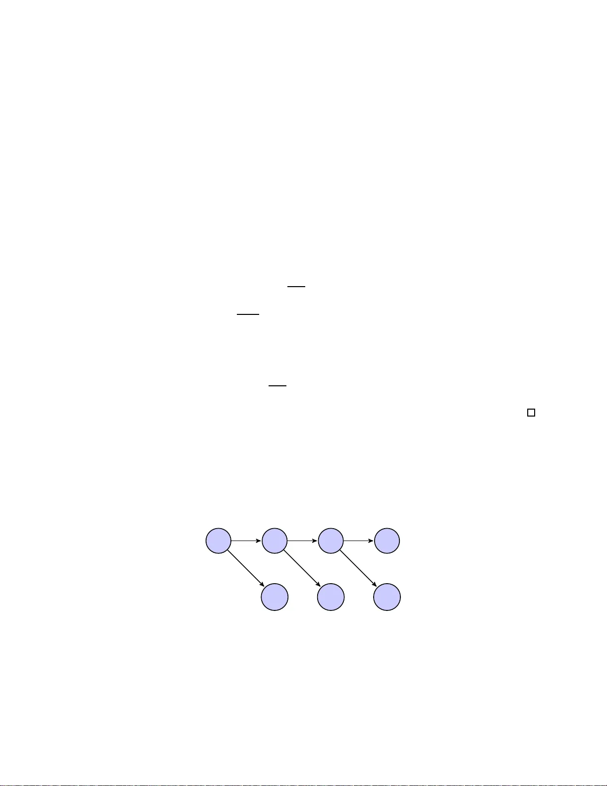
Shap e-constrained Estimation of V alue F unctions Mohammad Mousa vi ∗ , P eter W. Glynn † Septem b er 4, 201 8 Abstract W e present a fully nonparametr ic metho d to estimate the v alue function, via simulation, in the context of expected infinite-horiz o n discount ed r e wards for Marko v c hains. Estimating such v alue functions plays an imp ortant role in a pproximate dynamic progra mming . W e inco rp orate “soft information” in to the estimation algorithm, such as k nowledge of co n vexit y , monotonicity , or Lip chitz constants. In the presence of such infor mation, a nonparametric estimator f or the v alue function can be computed that is prov ably consistent as the simulated time horizo n tends to infinit y . As an applica tio n, we implement o ur method on price tolling agreement contracts in energy markets. ∗ Corresponding author. Department of Management Science & Engineering, Stanford U niversi ty , email: mousavi@st anford.edu , we b: www.stanfo rd.edu/ ∼ mousavi . † Department of Managemen t Science & Engineering, Stanford Universit y , email: glynn@stanford .edu , w eb: www.stanfo rd.edu/ ∼ glynn . 1 1 In tro duction This pap er is concerned with the estimation, via simula tion, of v alue functions in the con text of exp ected infinite horizon discounted r ew ards for Mark o v c hains. Estimating suc h v alue functions pla ys an imp ortant role in appr oximate d y n amic pr ogramming and applied pr obabilit y in general. In man y problems of p ractical in terest, the state space is huge or eve n contin uous and the v alue function is computatio nally intractable. Therefore, w e need to approximate the v alue fu n ction. In this w ork, w e dev elop a fully non-parametric metho d to estimate the v al ue function b y incorp orating shap e constrain ts, such as kno wledge of con ve xit y , monotonicit y , or Lipschitz constan ts. The most common metho d emp lo y ed to approximate the v al ue fu nction is parametric appro x- imate dynamic programming; see P o w ell (2011) and Bertsek as (2007 ). In this method , the user sp ecifies an “appro ximation arc hitecture” (i.e. a set of basis fu nctions) and the algorithm then pr o- duces an app ro ximation in the span of this basis. Selecting the basis function is essen tial b ecause an inapp ropriate “appr o ximation arc hitecture” m ight cause unsatisfactory resu lts, and cannot b e impro ve d by additional sampling or computational effort. In contrast, we are prop osing a fully “non-parametric” metho d to a v oid the difficult y of c ho os- ing a correct approxima tion arc hitecture. The general id ea is to take adv an tage of sh ap e p r op erties of th e optimal v alue f unction in estimating the fu nction. A v a riet y of con trol problems exist on con tin uous state spaces for wh ic h con v exit y in the v alue function naturally a rises. F or instance, in a linear tr ansition sys tem, if the rewa rd function in eac h stage is con ve x, then th e v alue fu nc- tion is con v ex. Inv en tory m o dels rep r esen t a w ell-kno wn example of this class of problems. S ingu- lar s to chastic con trol (Kumar and Muth uraman (2004)) and partially observed Marko v p ro cesses (Smallw o o d and Sondik (1973)) are t w o other s u b classes of problems for wh ic h the v alue f u nction is con v ex. As another example, Karoui et al. (1998) show that the American-st yle option is con v ex for a generalized Blac k–Sc holes mo del. Monotonicit y prop erties h a v e b een stu d ied in the literature for v arious p roblems formulated as Mark o v decision pr o cesses. F or instance, if the reward is monotone and the c hain is sto c hastically monotone, the v alue function is monotone. In P apadaki and P o we ll (2007), the monotonicit y of the v al ue fu nction is s tu died in the case o f the multi-prod uct b atc h disp atc h p roblem. Stok ey (1989, p. 267-268) presents general cond itions that guaran tee the v alue function will b e monotonic in the underlying stat e v ariable. Disc uss ions of monotonicit y appear also in Serfozo (19 76 ) and T opkis (1998). In Smith and McCardle (2002) and A tak an (2003), suffi cien t conditions are provided on the 2 transition probabilit y of a s to chastic dyn amic pr ogramming p r oblem to ensure the sh ap e prop erties of the v alue function. The goal of our work is to exploit this typ e of shap e p r op ert y to estimate the v al ue fu nction. W e s u ggest tw o metho ds for compu ting an appro ximation of the v alue fun ction for a fixed p olicy . In the first metho d, we estimate the v alue function along a p ath by explicitly incorp orating the shap e constrain t. F or in s tance, in the case that w e know the v alue function is con v ex, we consid er the set of all conv ex functions wh ic h is a con v ex cone in the space of measurable f unctions. Ha ving a sample path of the u nderlining pro cess, one can reac h a noisy observ ation of the v alue f unction. By pro jecting this n oisy observ at ion to the cone of con ve x functions, we ac hieve an estimator f or the v alue function. Since this metho d r equires only one sample path of th e pro cess, it can b e u s ed in reinforcemen t learning applications. The second metho d is b ased on estimating the v alue fu nction by taking adv an tage of th e fixed p oint prop erty of the v alue fun ction in ad d ition to the shap e constrain t. The v a lue function satisfies a sp ecific linear system of equations. Therefore, estimating the v alue function is p ossible by app ro x- imating the fixed p oint of this system of equations o v er th e cone o f conv ex functions. This fixed p oint can b e obtained by iterativ ely pro jecting on to the cone of con v ex fu n ctions. The simulatio n results show that the second approac h has reduced v ariance and provi des more accurate estimators as compared to the fi rst appr oac h. The pro jection onto the cone of conv ex functions is p ossible by solving a least squ are opti- mization problem. This optimizatio n pr oblem can b e in terpreted as a m ulti-dimensional con v ex regression. Con v ex r egression is concerned with computing the b est fit of a conv ex function to a dataset of n observ ations; Y i = f ( X i ) + ǫ i for i = 1 , . . . , n . Conv ex regression der ives a con v ex estimator of f by solving a least s q u are prob- lem. In one dimension, the theory of conv ex regression is well established; see Hanson and Pledger (1976) for the consistency result and Mammen (1991 ) and Gro eneb o om et al. (2001) for the rate of con v ergence. The consistency of conv ex r egression has b een shown in Lim and Glynn (2012), and in Seijo and Sen (2011) in the multi- dimensional case w h ere the observ ations are in dep endent. T o sho w the consistency of the estimator in our metho d, we extend the r esults in con ve x regression literature to the Marko v p ro cesses. Let X = ( X t : t ≥ 0) b e a p ositiv e Harris recurr en t and the noise sequence b e a correlated sequence satisfying su itable tec hnical assump tions. W e s ho w that the estima tor is con ve rging to the pro jection of f on to the cone of co nv ex f unctions in the 3 Hilb ert space of measurable functions. Lim and Glynn (2012) studied the b eha vior of the estimator when the mo del is mis-sp ecifed so th at the function f is non-con vex under the m uc h stronger assumption that the fu nction f is b ound ed. Our result relaxes this assumption. Recen tly , Hannah and Dun s on (2011 , 2013) employ ed the notion of fitting con v ex functions in solving dynamic programming problems. Th e k ey differences b et wee n our w ork and Hannah and Dunson (2013, 2011) are as follo ws: i.) Ou r m etho d is fully non-parametric wh ile their approac h is semi-parametric and required ad- justing sev eral parameters b efore fitting a con v ex fu nction or determinin g the prior distribution for Ba y esian up dating. ii.) Hannah and Dunson (2011, 2013) used the v alue iteration m etho d which inv olv es generating man y sample paths. In contrast , w e are using single or t w o sample paths. iii.) It is well kno wn that v alue iteration t yp e algorithms often lead to errors that gro w exp onen- tially in the pr oblem h orizon. Small lo cal c hanges at eac h iteration can lead to a large global error of the appro ximation; see S ection IV of Tsitsiklis and V an Ro y (2001 ) and Ma and P o w ell (2009). In con trast, in our metho d the pro jection to the con v ex s et o ccur s asymp totically w ith resp ect to the stationary distribu tion of the un d erlying Mark o v chain and has a con ve rgence guaran tee. The literature on approximate d ynamic programming (ADP) is also related to our w ork. Some recen t w orks in this area su ggest that the p erform ance of p arametric ADP algorithms is improv ed b y exploiting stru ctur al prop erties; see W ang and Judd (2000); Cai and Judd (2010, 2012a,b,c); Cai et al. (2013). In addition, God frey and P o w ell (2001) and P o w ell et al. (2004) consider the cases where the v alue functions are kno wn to b e conv ex and approxi mate the v alue fu nction by separable, piecewise linear functions of one v ariable. In Kunnumk al and T opaloglu (201 0 ), the monotonicit y of v al ue functions are used to appro ximate the v alue fu nction w h ere the state space is finite. In greater d etail, w e mak e the follo wing cont ribu tions: i.) W e rigorously devel op a fu lly non-parametric m etho d to estimate sh ap e constrained v alue functions of multi-dimensional con tin uous state space M.C. In the case that the v al ue function is con v ex, the estimator c an be r ep resen ted as a piecewise linear fu nction and ev aluated at eac h p oint in linear time. 4 ii.) W e extend the conv ex regression to the case in which explanatory v aria bles are sampled along a Mark o v c hain path. Moreo ver, the observ ations are corr elated and generated along the same path. iii.) W e iden tify the b eha vior of the estimator in the case of mis-sp ecification, wh ere the v alue function is n ot-con v ex. iv.) W e sh o w the con v ergence of the estimator to the solution of the p ro jected Bellman equation as the length of the sample path goes to infi nit y , v.) W e extend the non-parametric metho d to estimate the v alue functions whic h are Lipschitz or monotone and con v ex. The rest of this section is organized as follo ws: In S ection 2, w e precisely int ro d uce the mathematical framew ork for our analysis. In section 3, we describ e our metho d s. Section 4 pr esen ts the extension of m ulti-dimensional conv ex regression to the Mark o v pro cesses and shows the consistency of conv ex regression in this general framew ork. In Section 5, we use the results of Sectio n 4 to pro v e the con v ergence of our metho ds. In Section 6, we extend our m etho ds to estimate the v alue functions b y exploiting other shap e s tr uctures. In Section 7, w e study the efficacy of our metho ds by app lying them to a pr icing pr oblem in energy market. 2 F orm ulat ion Let X = ( X t : t ≥ 0) b e a discrete time Mark o v c hain ev olving on a general con tinuous state space X embedd ed on R d . E ach r andom v ariable X t is measurable with resp ect to the Borel σ -algebra asso ciated with R d . The transition probabilit y of the Marko v c hain P ( x, B ) represents the time- homogeneous probabilit y that the next state will b e X t +1 ∈ B giv en that the current state is X t = x . Let r ( X t ) b e the rew ard function receiv ed at time t , and e − α b e a discounti ng factor with α > 0. The v alue function, whic h is the exp ected infin ite horizon discounted rew ard for the Mark o v c hain, is giv en by V ∗ ( x ) = E " ∞ X t =0 e − tα r ( X t )    X 0 = x # . According to th e Mark o v pr op ert y , we h a v e V ∗ ( x ) = E h r ( X t ) + e − α V ∗ ( X t +1 )    X t = x i . 5 Define the op erator T : L ( X ) → R by ( T φ )( x ) = E h r ( X t ) + e − α φ ( X t +1 )    X t = x i , where L ( X ) is the space of measurable fu nctions o v er X . The op er ator T can b e considered as the Bellman op erator for a fixed p olicy . It is wel l known th at T is a con traction with r esp ect to the sup norm. k T φ − T φ ′ k ∞ ≤ e − α k φ − φ ′ k ∞ , for eve ry φ 1 , φ 2 ∈ L ( X ). F ur thermore, the v a lue function is th e unique fi xed p oint of equation V ∗ = T V ∗ ; see Bertsek as (2007 , p .408). Let π b e a probabilit y measure on R d . Define L 2 π = n φ : R d → R su c h that k φ k π < ∞ o where k φ k π =  Z x ∈ R d φ 2 ( x ) π ( dx )  1 / 2 . Supp ose th at C is the s et of all con ve x fun ctions o v er R d whic h are measurable with resp ect to π . Note th at C is a closed con v ex cone o v er th e sp ace of functions L 2 π ; s ee Lim and Glynn (2012). The pro jection op er ator onto th e cone C with resp ect to the measure π , repr esen ted b y Π C , is defin ed as Π C ( f ) = arg min φ ∈C k f − φ k π . The pro jection of f on to the con v ex cone C , d enoted by ¯ φ = Π C ( f ), can b e charact erized by h f − ¯ φ, φ − ¯ φ i π ≤ 0 for ev ery φ ∈ C . 3 Con v ex V alue Exploration In this section, we suggest t w o differen t metho ds to app r o ximate the v alue function f or a give n fixed p olicy by incorp orating the shap e constrain ts. Here, w e fir st f o cus on the con v exit y as a shap e constrain t. Next, w e extend our metho d s to monotonicit y and Lipschitz constrain ts. In th e first 6 metho d, we estimate the v alue function by explicitly incorp orating the shap e constraints. In the second one, w e impro ve the estimator b y incorp orating the sh ap e constrain t and sim ultaneously taking adv an tage of the fact that the fun ction satisfies a sp ecific linear sy s tem of equ ations. In the subsequent sections, w e discuss the con v ergence of th ese metho ds. 3.1 T runcated Method Let X = ( X t : t ≥ 0) b e the u nderlying Marko v pro cess. Consid er a s in gle sample path of X . The total discounte d r ewards ov er this sample p ath rise to noisy obs er v ations of th e v alue fun ction at these sample p oin ts. Fitting a con v ex function to these observ ations giv es an estimation of the v al ue function. S ince we trun cate the infinite horizon discounted rew ard str eam to get th e noisy observ ati on at eac h s ample p oin t, we call this metho d th e trunc ate d metho d . Let X 1 , X 2 , . . . , X 2 N b e a sample path of the Marko v chain with length 2 N . Also, assume that R 1 , . . . , R 2 N is the s equence of corresp ondin g rewa rd s at sample p oin ts R i = r ( X i ) f or 1 ≤ i ≤ 2 N . A n oisy observ at ion of V ∗ ( X i ) is thus give n by Y N i = 2 N X i = j e − ( j − i ) α R j (1) for 1 ≤ i ≤ N . Observe that Y N i = V ∗ ( X i ) + ǫ i , w here E [ ǫ i | X i ] is close to zero if th e num b er of sample points N is su fficien tly large. W e can constru ct an estima tor of V ∗ ( x ) by pro jecting the noisy observ atio ns on to the cone of con v ex fun ctions. T h e pro jection is p ossible by fitting a conv ex function to the p oin ts ( X 1 , Y N 1 ) , . . . , ( X N , Y N N ). Assuming V ∗ ( x ) is a conv ex function, we use the least squares estimator (LSE) to p ro ject th e noisy observ atio ns onto the cone of conv ex fun ctions b y solving min φ ∈C N X i =1 ( Y N i − φ ( X i )) 2 . (2) Since C is an infi nite-dimensional space, th is minimization ma y app ear to b e computationally in tractable. Ho we ve r, it turn s out that this min imization can b e f orm ulated as a finite-dimensional 7 quadratic program (QP): min p i ,ζ i N X i =1 ( Y N i − p i ) 2 p i ≥ p j + ζ T j ( X i − X j ) for ev ery 1 ≤ i, j ≤ N . (3) In Lim and Glynn (2012), it is s h o wn that this least square problem has a minimizer ( p 1 , ζ 1 ) , . . . , ( p n , ζ n ), and an y m inimizer φ N of (2) ov er C sat isfies φ N ( X i ) = p i . W e defer more discussion of solving this optimization problem more efficien tly to Chapter 5. W e defin e our estimator V N ( x ) as V N ( x ) = sup n φ ( x ) : φ ∈ C , φ ( X i ) = p i , i = 1 , . . . , N o . The function V N is a con v ex an d finite v alue fun ction o ve r the con v ex h ull of the p oints ( X 1 , . . . , X N ). F ur thermore, it is s traigh tforw ard to show that V N is a p iecewise linear conv ex function giv en by V N ( X ) = max 1 ≤ i ≤ N ( p i + ζ T i ( X − X i )) . (4) In the n ext sect ion, we w ill sho w that a s the sample size N → ∞ , the estimator V N con v erges uniformly to V ∗ o v er every compact set. 3.2 Fixed P oin t Pro jection In th is section, we impro ve the previous m etho d by taking adv an tag e of the fixed p oint prop erty of the v alue fu nction in addition to the shap e constrain t. The r ationale of the metho d is to iterativ ely apply the Bellman op erator T and pro ject to the cone of conv ex fun ctions. This metho d p ro vides an appr o ximation of the v alue function as the fi xed p oint of the op erator T . First, w e start with the ideal case, in whic h w e can exa ctly compute the expectation with resp ect to the stationary distribution as w ell as the pro jection to the sp ace of con v ex fun ctions. Next, we explain a n umerical algorithm that app ro ximately follo ws th is id eal iteration pr o cedure. Here, w e assume the v alue function belongs to the space of measurable functions L 2 π and is con v ex. In the next section, w e study the b eha vior of the estimator in the general case where the v al ue fun ction is not con v ex. Th e v alue fun ction is the fixed p oin t of th e op erator T , so V ∗ = T V ∗ . Moreo v er, by the con ve xit y assump tion, V ∗ is a fi xed p oin t of th e pro jection op erator on to the cone of con v ex functions, and we h a v e V ∗ = Π C V ∗ . Therefore, V ∗ is the fixed p oin t of the combinatio n 8 of the op erators T and Π C and satisfies V ∗ = Π C T V ∗ . In th e next theorem, w e s h o w the existence of su c h a fixed p oint as a result the of con tractio n of b oth op erators T and Π C . Theorem 3.1. L et π b e the stationary distribution of the Markov chain X , and r ∈ L 2 π . Then ther e exists a uni q ue fixe d p oint V ∈ L 2 π such that V = Π C T V . Mor e over, let V = ( V k ; k ≥ 0) b e a se quenc e of functions in the c onvex close d c one C ⊂ L 2 π , define d by V k +1 = Π C T V k . (5) Then, we have k V k − V k π ≤ e − k α k V 0 − V k π . Remark 3.2. The se qu e nc e V = ( V k : k ≥ 0) gener at e d in (5) do es not c onver ge for an arbitr ary norm k · k π . The assumption that π is the stationary distribution of the underlying M arkov chain X is essential to guar ante e the c onver genc e of the se quenc e. F or instanc e, the pr oje ction with r esp e ct to the sup -norm is not c ontr action (se e Exampl e B.1). F or a similar discussion in the c ontext of p ar ametric ADP, se e Tsitsiklis and V a n R oy (2001). Pr o of. First, we s ho w that if π is th e stationary distrib ution of the Mark o v c hain, then the op erator T is a con traction with resp ect to the norm k · k π . F or any tw o fu nctions φ 1 , φ 2 ∈ L 2 π , we h av e E π ( T φ 1 − T φ 2 ) 2 = E π  E [ r ( X t ) + e − α φ 1 ( X t +1 ) | X t ] − E [ r ( X t ) + e − α φ 2 ( X t +1 ) | X t ]  2 = e − 2 α E π  E [ φ 1 ( X t +1 ) − φ 2 ( X t +1 ) | X t ]  2 ≤ e − 2 α E π  φ 1 ( X t +1 ) − φ 2 ( X t +1 )  2 = e − 2 α k φ 1 − φ 2 k 2 π . 9 Moreo v er, we kno w that Π C , the pr o jection op erator ont o th e con v ex cone C , is also a con traction with resp ect to k · k π norm; see P .26 Borw ein and Lewis (2005). More precisely , if φ 1 , φ 2 ∈ L 2 π ( X ), then w e ha v e k Π C φ 1 − Π C φ 2 k π ≤ k φ 1 − φ 2 k π . Note that E π  r ( X t ) + e − α E [ φ ( X t +1 ) | X t ]  2 ≤ 2 E π r ( X t ) 2 + 2 e − 2 α E π φ ( X t +1 ) 2 < ∞ . Th us, T φ ∈ L 2 π for ev ery φ ∈ L 2 π . Therefore, k Π C T φ 1 − Π C T φ 2 k π ≤ e − α k φ 1 − φ 2 k π . The rest of the theorem follo ws d irectly from the Banac h fixed p oin t theorem. In the rest of this section, we d ev elop a computational metho d to appr o ximate the fixed p oin t o v er the cone C b y using simula ted tra jectories. Exact compu tation of T V is n ot generally viable. Ev aluat ing T V ( x ) at any x ∈ X inv o lve s the computation of the exp ectation E [ V ( X t +1 ) | X t = x ] . This exp ectatio n is ov er a p oten tially h igh-d imensional or infin ite-dimensional space and hen ce can p ose a computational c hallenge. The follo wing pr op osition p ro vides an equiv ale nt c haracterizati on to the op erator Π C T . As a result of this p rop osition, it suffices to ev aluate V ( · ) at tw o sample p oin ts rather than compu ting E [ V ( X t +1 ) | X t = x ] . Prop osition 3.3. L et X t +1 and e X t +1 b e two indep endent samples of an M.C. at time t + 1 given X t . Mor e over, define the r andom variable H t such that H t = r ( X t ) + e − α 2  V ( X t +1 ) + V ( e X t +1 )  . (6) F or every me asur able function V ∈ L 2 π , we have Π C T V = arg min φ ∈C E π  H t − φ ( X t )  2 . Ther efor e, Π C T V = Π C H . Pr o of. Let ¯ φ b e the pr o jection of T V on to the cone of conv ex functions C , wh ic h is the minimizer 10 of min φ ∈C E π ( T V − φ ) 2 . By using the ind ep endence of X t +1 and e X t +1 giv en X t , we obtain E π ( T V − φ ) 2 = E π  E [ r ( X t ) + e − α V ( X t +1 ) | X t ] − φ ( X t )  2 = E π h E [ r ( X t ) + e − α V ( X t +1 ) − φ ( X t ) | X t ]  (7) ×  E [ r ( X t ) + e − α V ( e X t +1 ) − φ ( X t ) | X t ] i = E π h r ( X t ) + e − α V ( X t +1 ) − φ ( X t )  ×  r ( X t ) + e − α V ( e X t +1 ) − φ ( X t ) i = E π h r ( X t ) + e − α 2 ( V ( X t +1 ) + V ( e X t +1 )) − φ ( X t )  2 − e − 2 α 4  V ( e X t +1 ) − V ( X t +1 )  2 i (8) for eve ry fu nction φ ∈ L 2 π . T herefore, we can conclude that ¯ φ is also the minimizer of the optimiza- tion ¯ φ = arg min φ ∈C E π  r ( X t ) + e − α 2  V ( X t +1 ) + V ( e X t +1 )) − φ ( X t )  2  . By u sing the ergo dic prop erty of th e Marko v chains, it is str aigh tforw ard to calculate an esti- mator of E π ( H t − φ t ) 2 . At eac h time step t = 1 , . . . , N , we generate tw o ind ep endent copies X t +1 and e X t +1 giv en X t . W e call ( X 1 , X 2 , e X 2 , . . . , X N +1 , e X N +1 ) a “two c opy sample p ath” . Figure 1: A two c opy sample p ath of length 4 X 1 X 2 e X 2 X 3 e X 3 X 4 e X 4 11 Under appropriate conditions o v er the pro cess X , w e ha ve 1 N N X t =1 ( H t − φ ( X t )) 2 → E π ( H t − φ ( X t )) 2 as N → ∞ . Here, we d iscuss a p otenti al but un successful Mon te C arlo approac h to ap p ro ximate V ∗ . By th e con v exit y assump tion, th e v alue fun ction is the fix ed p oin t of V ∗ = Π C T V ∗ , and therefore is the minimizer of the optimizatio n problem min φ ∈C k φ − Π C T φ k 2 π . Similar to Pr op osition 3.3, it is p ossible to sh o w that the fixed p oin t V ∗ is also the m in imizer of min φ ∈C E π h r ( X t ) + e − α φ ( X t +1 ) − φ ( X t )  r ( X t ) + e − α φ ( e X t +1 ) − φ ( X t ) i . One migh t solv e the optimization prob lem min φ ∈C 1 N N X t =1  r ( X t ) + e − α φ ( X t +1 ) − φ ( X t )  r ( X t ) + e − α φ ( e X t +1 ) − φ ( X t )  . (9) Ho w ev er, it can b e easily sho wn th at this op timization p r oblem is non -conv ex and unb ounded for an y finite sample path of length N ; see Example B.2. W e can solv e this d ifficult y by emplo ying an iterativ e pro j ection p ro cedure. Before discussing this m etho d, w e imp ose an ad d itional shap e con- strain t to b ound the v alue fu nction. This assump tion helps to restrict the cone of conv ex functions and mak e the pro jection more tractable. Assumption 3.4. L et the state sp ac e X b e b ounde d. Mor e over, assume that for every x ∈ X , the sub-gr adient of V ∗ is b ounde d by a c onstant K : k∇ V ( x ) k ∞ < K, and V (0) > − K . Example 3.5. Supp ose that ther e exists a c onstant K such that for every state x ∈ X we have    r ( x ) − E [ r ( X 1 ) | X 0 = x ]    ≤ K. 12 It i s str aightfo rwar d to show that    V ∗ ( x ) − r ( x ) 1 − e − α    ≤ K (1 − e − α ) 2 . Ther efor e, if the r ewa r d function is b ounde d over the state sp ac e, then Assu mption (3.4) holds. No w, w e present an alternativ e metho d to estimate the v alue fun ction by u sing conv exit y and the fixed p oint p r op ert y . The metho d is similar to the ideal pro cedure in Th eorem 3.1. The main difference is u sing the random v ector ˆ H k = ( ˆ H k 1 , . . . , ˆ H k N ) for a piecewise linear function ˆ V k ( · ) instead of T ˆ V k . W e fi rst generate a two c opy sample p ath of length N . This samp le path do es not c hange throughout th e pro cedu re. W e iterativ ely compute the ran d om vecto r ˆ H k = ( ˆ H k 1 , . . . , ˆ H k N ) for a piecewise linear fu nction ˆ V ( · ). Next, w e p ro ject ˆ H k on to the con v ex cone C to ac hiev e ˆ V k +1 . Eac h con v ex pr o jection is a least square finite-dimensional optimization p roblem. By follo wing this pro cedure iterativ ely , an estimation of the fixed p oin t ov er the cone C is obtained. The details of the metho d are as follo ws: Algorithm Fixed P oin t Pro jection Input: N and ǫ Output: Th e estimator of the v al ue fu nction ˆ V k . Initialize: Select a piecewise-linear fu nction V 0 ( x ), and set k = 0, V − 1 ( x ) = 0. Generating Sample P ath: Generate a “t w o copy s ample p ath” of length N + 1. while k ˆ V k − ˆ V k − 1 k ˜ π N > ǫ do i.) Comp ute ( H k t ) N t =1 from (10). ii.) Pro j ect ( H k t ) N t =1 b y solving the optimization problem (11), and find ( p i , ζ i ) for i = 1 . . . , N . iii.) Up date ˆ V k +1 ( · ) thorough (12), and k ← k + 1. end w hile return The piecewise-linear fun ction ˆ V k . Generating Sample Path: Generate a “two c opy sample p ath” of length N + 1. A t eac h ti me step t = 1 , . . . , N , generate t wo indep endent copies X t +1 and e X t +1 giv en X t . Up dating Step: Ev aluate ˆ H k t = r ( X t ) + e − α 2 ( ˆ V k ( X t +1 ) + ˆ V k ( e X t +1 )) (10) 13 for ev ery t = 1 , . . . , N . The sequ ence ˆ H K = ( ˆ H k 1 , . . . , ˆ H k N ) is a noisy observ ation of T ˆ V k ( X t ). Pro jection: Pr o ject ˆ H k on to the cone of con v ex functions by s olving the finite-dimensional conv ex program min 1 N N − 1 X t =0 ( ˆ H k t − p t ) 2 (11) p i ≥ p j + ζ T j ( X i − X j ) for ev ery 1 ≤ i, j ≤ N − K ≤ ζ l j ≤ K for ev ery i = 1 , . . . , N , and l = 1 , . . . , d − K ≤ p j + ζ T j X i . Giv en the optimal solution ( p t , ζ t , X t ) N t =1 to this optimizatio n, w e can construct a piecewise linear con v ex fu nction. Define ˆ V k +1 ( x ) = max 0 ≤ i ≤ N ( p i + ζ T i ( x − X i )) . (12) The u p dating and pro jection stages for a fixed “two c opy sample p ath ” should b e conti nued until a desired lev el of accuracy is r eac hed. W e can consider ˆ V k ( x ) as an estimator for the v alue fu n ction. In the next s ection, we will sh o w that for sufficien tly large sample size N a nd a large num b er of itera- tions k , the estimator ˆ V k ( x ) con v erges uniform ly to th e v alue fu nction V ∗ ( x ) o v er ev ery compact set. 4 Empirical Pro jection Consistency In this section w e describ e a generalization of the consistency result of con ve x regression in Lim and Glyn n (2012) to the p ositiv e Harris c hains. Our result includ es the mo del mis-sp ecificatio n case w ithout an y extra assumption to b ound the fu nction. In the n ext section, we use this r esult to sho w that the estimators in trunc ate d metho d and fixe d p oint pr oje ction metho d con ve rge to the v alue fu nction as the sample s ize grows to infi nit y . Let X = ( X t : t ≥ 1) b e defin ed on the probabilit y space (Ω , F , P ). F or ev ery F -measurable random v a riable Y , w e can define the pr o jection onto the cone C with r esp ect to the norm π as the solution of min φ ∈C E π ( Y − φ ( X )) 2 . 14 Let ( Y N i : 1 ≤ i ≤ N , 1 ≤ N ) b e a sequence of random v ectors in wh ic h Y N = ( Y N 1 , . . . , Y N N ) f or ev ery N ≥ 1. W e sho w th at if ( Y N : N ≥ 1) c o nver ges on aver age to Y , then the empirical pr o jection of this sequence ont o the cone of conv ex fun ctions giv es a consisten t estimate of pro jecting Y on to this cone. F or ease of exp osition, we define a sequence of random vecto rs as str ongly er go dic in the follo wing wa y : Definition 4.1. Supp ose that X = ( X t : t ≥ 1) is a p ositive Harris chain with stationary dist ri- bution π , and ( Y N t : 1 ≤ N , 1 ≤ t ≤ N ) b e a se quenc e of r andom variables. We c al l this se quenc e “str ongly er go dic” if ther e exists a F - me as ur able r andom v ariable Y such that E Y 2 < ∞ , 1 N N X t =1 ( Y N t − g ( X t )) 2 I ( k X t k ≤ c ) → E π ( Y − g ( X t )) 2 I ( k X k ≤ c ) a.s. for eve ry fu nction g ∈ L 2 π , and c ≤ ∞ . T o illustr ate this definition, we p ro vide sev eral examples. Example 4.2. L et the Y N t = f ( X t ) + ν t b e suc h that ν t is a se quenc e of i.i.d noise terms with r e sp e ct to X such that E ν 2 t < ∞ , and f is a c onvex function in C . Then by the str ong law of lar ge numb ers, we obtain that ( Y N : N ≥ 1) is “str ongly er go dic”. Example 4.3. In L emma A.2, we show that if E π r ( X t ) 2 < ∞ , then the two f ol lowing r andom se quenc es ar e “str ongly er go dic”: Y N t = ∞ X j = t e − ( j − t ) α r ( X j ) , Y N t = 2 N X j = t e − ( j − t ) α r ( X j ) . Example 4.4. Assume that ( X t , e X t ) is a “two c opy sample p ath” of a Harris r e curr ent chain. L et V ∈ L 2 π and as we define d in (10), H N t = r ( X t ) + 1 2 ( V ( X t +1 ) + V ( e X t +1 )) . Then, ( H N : N ≥ 1) i s a “str ongly er go dic” se quenc e; se e L emma A.3. 15 Let g N b e the optimizer of the con v ex optimization problem min g ∈C 1 N N X t =1 ( Y N t − g ( X t ) 2 ) (13) for N ≥ 1. Note that similar to (11), we can conv ert this optimization problem to a fi nite quadratic con v ex pr oblem. In the f ollo wing theorem, we sho w that g N is an estimator for g ∗ , th e pro j ection of Y ont o the space of con v ex fu nctions. W e need some assumptions ov er the structure of the Marko v c hain. Assumption 4.5. F or the Markov chain X , we have: i.) It is p ositive Harris r e curr ent with unique stationary distribution π . ii.) π ( B ) > 0 for every p ositive r adius b al l B which is a subset of state sp ac e X . iii.) E π X 2 t < ∞ . Theorem 4.6. Assume that ( Y N : N ≥ 1) is “str ongly er go dic”, and Assumption (4.5) hold s. L et g N b e the solution of (13) and g ∗ ∈ C b e the uniq u e minimizer of min g ∈C E π ( Y − g ( X )) 2 . Then, 1 N N X t =1 ( g N ( X t ) − g ∗ ( X t )) 2 → 0 a.s. as N → ∞ . Mor e over, sup k x k≤ c | ˆ g n ( x ) − g ∗ ( x ) | → 0 a.s. as N → ∞ , for every c > 0 . The pro of follo ws the same steps as the con v ergence pro of in Lim an d Glynn (2012). The main difference is th e use of the er go d ic prop ert y of Harris chains instead of the s trong la w of large n umb er for i.i.d rand om v ariables. Moreo v er, w e con tinue to allo w the mo d el mis-sp ecification in whic h f ( X ) = E ( Y | X ) is not a con v ex fu nction. W e firs t start by sh owing the consistency of the pro jection onto the compact disk H c = { X : k X k ≤ c } for every c > 0. T hen, by expan d ing this pro jection ov er the whole s pace, w e conclude the theorem. 16 F or ev ery c > 0, d efine C c as the set of all fun ctions g ∈ L 2 π suc h that g is a conv ex function o ve r the disc { X : k X k ≤ c } . Similar to Prop osition 3 in Lim and Glynn (201 2 ), we can show th at C c is a closed subset of g ∈ L 2 π . Therefore, there exists a un ique function g ∗ c ∈ C c whic h is the pr o j ection of Y ont o C c . min g ∈C 2 c E π ( Y − g ) 2 It is clear that g c ( x ) = E [ Y | X = x ] for almost every x / ∈ H c . In Lemma A.1 , we sh o w g ∗ c con v erges to g ∗ as c goes to infi nit y . Pr o of of The or em 4.6 . Similar to the steps 1, 2, and 3 in Lim and Glynn (2012), w e ha v e 1 N N X i =1 ( g N ( X i ) − g ∗ ( X i )) 2 ≤ 2 N N X i =1 ( Y N i − g ∗ ( X i ))( g N ( X i ) − g ∗ ( X i )) , (14) and for s ufficien tly large N 1 N N X i =1 ( g N ( X i )) 2 ≤ 8 N N X i =1 ( Y N i − g ∗ ( X i )) 2 + 2 N N X i =1 ( g ∗ ( X i )) 2 ≤ 9 E π ( Y − g ∗ ( X )) 2 + 3 E π g ∗ ( X i ) 2 = β . (15) W e conclude the last inequalit y from the “str ongly er go dic” pr op ert y of ( Y N : N ≥ 1). By the Cauc hy– Sch w arz inequ ality , the tail of the emp irical inner pr o duct can b e uniformly b ou n ded for ev ery c > 0 and su ffi cien tly large N . Ob serv e that 1 N N X i =1 ( Y N i − g ∗ ( X i ))( g N ( X i ) − g ∗ ( X i )) I ( k X i k > c ) ≤  1 N N X i =1 ( g N ( X i ) − g ∗ ( X i )) 2  1 / 2  1 N N X i =1 ( Y N i − g ∗ ( X i )) 2 I ( k X i k > c )  1 / 2 ≤ ( β + 2 E π ( g ∗ ( X )) 2 ) 1 / 2 2  E π ( Y − g ∗ ( X )) I ( k X k > c )  1 / 2 . In the last line, w e used the “str o ngly er go dic” assumption and the tr iangle inequ alit y . S ince E π Y 2 < ∞ and E π g ∗ ( X ) 2 < ∞ , the r igh t hand side can b e smaller than any ǫ > 0 for large enough c . Thus, lim N →∞ 1 N N X i =1 ( Y N i − g ∗ ( X i ))( g N ( X i ) − g ∗ ( X i )) I ( k X i k > c ) ≤ ǫ (16) for sufficient ly large c . Therefore, the terms in (14), whic h corresp on d to the samples outside the 17 disk H c can b e made arb itrarily small. In the n ext lemma, we sho w that g N con v erges to g ∗ c inside the disk. Lemma 4.7. Then for every c > 0 , lim s up N →∞ 1 N N X i =1 ( Y N i − g ∗ c ( X i ))( g N ( X i ) − g ∗ c ( X i )) I ( k X i k < c ) ≤ 0 . See th e App endix for the pr o of. Th is lemma ens u res that there exists a sequence δ N con v erging to zero su c h that δ N ≥ 1 N N X i =1 ( Y N i − g ∗ c ( X i ))( g N ( X i ) − g ∗ c ( X i )) I ( k X i k < c ) = 1 N N X i =1  ( Y N i − g ∗ ( X i )) + ( g ∗ ( X i ) − g ∗ c ( X i ))  ×  ( g N ( X i ) − g ∗ ( X i )) + ( g ∗ ( X i ) − g ∗ c ( X i ))  I ( k X i k < c ) = 1 N N X i =1 ( Y N i − g ∗ ( X i ))( g N ( X i ) − g ∗ ( X i )) I ( k X i k < c ) (17) + 1 N N X i =1 ( Y N i − g ∗ ( X i ))( g ∗ ( X i ) − g ∗ c ( X i )) I ( k X i k < c ) (18) + 1 N N X i =1 ( g ∗ ( X i ) − g ∗ c ( X i ))( g N ( X i ) − g ∗ ( X i )) I ( k X i k < c ) (19) + 1 N N X i =1 ( g ∗ ( X i ) − g ∗ c ( X i )) 2 I ( k X i k < c ) . (20) W e can get a lo wer b ound for (18) by th e Cauch y–Sc h w arz inequ alit y . 1 N N X i =1 ( Y N i − g ∗ ( X i ))( g ∗ ( X i ) − g ∗ c ( X i )) I ( k X i k < c ) ≥ − 2( E π ( Y − g ∗ ( X )) 2 ) 1 / 2 ( E π ( g ∗ ( X ) − g ∗ c ( X )) 2 I ( k X k < c )) 1 / 2 for sufficient ly large N . Similarly , we can get a low er b ound for (19) by u sing (15) and Cauch y- Sc hw arz inequalit y 1 N N X i =1 ( g ∗ ( X i ) − g ∗ c ( X i ))( g N ( X i ) − g ∗ ( X i )) I ( k X i k < c ) 18 ≥ − 1 N N X i =1 ( g N ( X i )) 2 ! + N X i =1 ( g ∗ ( X i )) 2 !! 1 / 2 × 1 N N X i =1 ( g ∗ ( X i ) − g ∗ c ( X i )) 2 I ( k X i k < c ) ! 1 / 2 ≥ − 2  β + E π ( g ∗ ( X )) 2  1 / 2  E π ( g ∗ ( X ) − g ∗ c ( X )) 2 I ( k X k < c )  1 / 2 By com bining these inequalities and using Lemma 4.7, we obtain 1 N N X i =1 ( Y N i − g ∗ ( X i ))( g N ( X i ) − g ∗ ( X i )) I ( k X i k < c ) ≤ δ ( N ) + β 1 min { ( E π ( g ∗ ( X ) − g ∗ c ( X )) 2 I ( k X k < c )) 1 / 2 , 1 } . According to L emm a A.1, there exists a sufficient ly large c f or every ǫ > 0 suc h that E π ( g ∗ ( X ) − g ∗ c ( X )) 2 I ( k X k < c ) ≤ ǫ ′ . Therefore, there exists a sufficien tly large c for any ǫ > 0 such that 1 N N X i =1 ( Y N i − g ∗ ( X i ))( g N ( X i ) − g ∗ ( X i )) I ( k X i k < c ) ≤ ǫ. No w, w e can use (14) and (16) to conclud e the theorem. lim N →∞ 1 N N X i =1 ( g N ( X i ) − g ∗ ( X i )) 2 ≤ 1 N N X i =1 ( Y N i − g ∗ ( X i ))( g N ( X i ) − g ∗ ( X i )) I ( k X k < c ) + 1 N N X i =1 ( Y N i − g ∗ ( X i ))( g N ( X i ) − g ∗ ( X i )) I ( k X k > c ) ≤ 2 ǫ. The second p art of the theorem is similar to Step 8 in Lim and Glynn (2012). 19 5 Con v ergence of the V alue F unction Estimator In th is section we show that the estimators giv en by the trunc ate d metho d and the fixe d p oint pr oje ction metho d conv erge to the v alue fun ction as th e sample size grows to infinity . Th e con ve r- gence of th e tru ncated metho d h olds for a general setting. Ho w ev er, w e sh o w the con v ergence of the estimator giv en b y t he fixe d p oint pr oje ction metho d u nder Assum ption (3.4) o v er t he v alue function. Theorem 5.1. L et Y N t = 2 N X j = t e − ( i − t ) α R j , and V N ( x ) b e the estimator of trunc ate d metho d define d by (4). Assume that (4.5) holds. Then, we have sup k x k n . Therefore, k f − g ∗ m k 2 is an increa sing b ounded sequence. It follo ws th at W = lim m →∞ | f − g ∗ m k 2 π for some W < k f k 2 π . S ince k f − g ∗ m k 2 π − k f − g ∗ n k 2 π ≥ k g ∗ m − g ∗ n k 2 π for m ≥ n , ( g ∗ n ) is a C auc h y sequence in L 2 π . Therefore, g ∗ n con v erges to g ∞ in L 2 norm. This im p lies that there is a sub-sequence g ∗ n k con v erging almost surely to g ∞ . Let x, y ∈ R d , and 0 < θ < 1. Then, g ∗ n k ( θ x + (1 − θ y ) y ) ≤ θ g ∗ n k ( x ) + (1 − θ ) g ∗ n k ( y ) for ev ery n k > max( x, y ). Since, g ∗ n k con v erges almost surely to g ∞ as n k go es to infinit y , g ∞ is a con v ex fu nction in L 2 π , from wh ic h we conclud e th at g ∞ ∈ C . No w, w e sh ow th at g ∞ is the pro jection of f o v er C . Every con v ex function φ ∈ C is conv ex ov er H c , so φ ∈ C m for ev ery m . T h us h f − g ∗ n , φ − g ∗ n i π ≤ 0 . 33 Since k g ∗ n − g ∞ k π → 0, it easy to sho w that h f − g ∞ , φ − g ∞ i π ≤ 0 . This equalit y h olds for ev ery φ ∈ C . As a resu lt, we can conclude that g ∞ is the pro jection of f ov er C . According to the conv exit y of C , the pro jection of f is u nique and equal to g ∗ . Thus, g ∞ = g ∗ almost everywhere, and we h a v e k g ∗ n − g ∗ k π → 0 . Lemma 4.7. Then for every c > 0 , lim s up N →∞ 1 N N X i =1 ( Y N i − g ∗ c ( X i ))( g N ( X i ) − g ∗ c ( X i )) I ( k X i k < c ) ≤ 0 . Pr o of of Lemma 4.7 . Replacing the g N with a fixed con v ex f unction ˜ g n ot d ep endent on N , sho wing the lemma is straigh tforwa rd . The right -hand a ve rage w as conv erging to th e inn er pro duct h Y − g c , ˜ g − g c i π . S ince, g c is pro jection of Y to the close conv ex set C c , th is inner pro du ct is n egativ e. Ho w ev er, this argument f ails for g N since it dep en d s on N . T o fix this difficult y , we sho w that it is p ossib le to appro ximate ev ery function g N b y a memb er o f a finite set of con ve x fu nctions o v er H c . So, th e limit is b ounded with a corr esp onding limit f or a fi xed con v ex function whic h is asymptotically negativ e according to the pro jection prop er ty . By Assumption 4.5 , w e ha v e π ( X ∈ B ) > 0 for ev ery compact disc B , and (15 ) en sures that 1 N N X i =1 g N ( X i ) 2 ≤ β . Similar to Prop osition 4 in Lim and Glynn (2012), it is p ossible to show that for eac h c > 0, there exists a deterministic γ ( c ), su ch that g N is Lipsc hitz o v er H c with factor γ ( c ) for su fficien tly large N . It follo ws that for ev ery ǫ > 0, th er e exists a finite collection of con ve x fun ctions h 1 , h 2 , . . . , h m whic h is ǫ -net for C c (1+ δ ) ; for eve ry large N there exists some h k suc h that sup x ∈H c | g N ( x ) − h k ( x ) | ≤ ǫ ; 34 see Theorem 6 of Bronshtein (1976). If h k and g N satisfy this prop erty , observe that 1 N N X i =1 ( Y N i − g ∗ c ( X i ))( g N ( X i ) − g ∗ c ( X i )) I ( k X i k < c ) ≤ 1 N N X i =1 ( Y N i − g ∗ c ( X i ))( g N ( X i ) − h k ( X i )) I ( k X i k < c ) + 1 N N X i =1 ( Y N i − g ∗ c ( X i ))( h k ( X i ) − g ∗ c ( X i )) I ( k X i k < c ) ≤ s u p x ∈H c | g N ( x ) − h k ( x ) | 1 N N X i =1 | Y N i − g ∗ c ( X i ) | I ( k X i k < c ) + max 1 ≤ k ≤ m 1 N N X i =1 ( Y N i − g ∗ c ( X i ))( h k ( X i ) − g ∗ c ( X i )) I ( k X i k < c ) ≤ ǫ ·  1 N N X i =1 | Y N i − g ∗ c ( X i ) | 2 I ( k X i k < c )  1 / 2 + max 1 ≤ k ≤ m 1 N N X i =1 ( Y N i − g ∗ c ( X i ))( h k ( X i ) − g ∗ c ( X i )) I ( k X i k < c ) Because h k ’s are b ounded ov er H c , and ( Y N i ) is “ str ongly er go dic” , 1 N N X i =1 ( Y N i − g ∗ c ( X i ))(( h k ( X i ) − g ∗ c ( X i ))) I ( k X i k < c ) → E π ( Y − g ∗ c ( X ))( h k ( X ) − g ∗ c ( X )) I ( k X k < c ) ≤ 0 as N → ∞ . Here, w e use the fact that g ∗ c is the pr o j ection of Y to C c , and h k is also a b ound ed con v ex fu nction ov er H c . As a r esu lt, lim N →∞ 1 N N X i =1 ( Y N i − g ∗ c ( X i ))( g N ( X i ) − g ∗ c ( X i )) I ( k X i k < c ) ≤ ǫ  E π | Y N i − g ∗ c ( X i ) | 2 I ( k X i k < c )  1 / 2 for ev ery ǫ > 0. Th is en s ures the lemma. Lemma A.2. L et X = ( X t : t ≥ 0) b e a Harris er go dic chain. A ssume that E π r ( X t ) 2 < ∞ . Then 35 the fol lowing two r an dom se que nc es ar e “str ongly er go dic”: Y t = ∞ X j = t e − ( j − t ) α r ( X t ) Y N t = 2 N X j = t e − ( j − t ) α r ( X t ) . Pr o of. Since X is a Harris ergo d ic c hain, there exists a s tationary p ro cess ˆ X in itialize d by in v arian t measure π and a fin ite coupling time T such that X t = ˆ X t for all t ≥ T ; see Prop osition 3.13 in Asm ussen (2003, Chapter VI I). Let ˆ Y t = ∞ X j = t e − ( j − t ) α r ( ˆ X t ) for t ≥ 0. F or ev ery g ∈ L 2 π , w e ha v e 1 N N X t =1 ( ˆ Y t − g ( ˆ X t )) 2 I ( k ˆ X t k ≤ c ) → E π ( ˆ Y − g ( ˆ X t )) 2 I ( k X k ≤ c ) a.s. b y the Birkh off–Khinc hin theorem; see C orollary 6.23 in Br eiman (1992, p.115). Moreo v er, we can easily sho w that 1 N T X t =1    ( ˆ Y t − g ( ˆ X t )) 2 − ( Y t − g ( X t )) 2    I ( k ˆ X t k ≤ c ) → 0 as N → ∞ . Therefore, by using the fact that X t = ˆ X t for all t ≥ T , we conclude that 1 N N X t =1 ( Y t − g ( X t )) 2 I ( k X t k ≤ c ) → E π  ( Y − g ( X t )) 2 I ( k X k ≤ c )  a.s. as N → ∞ . Therefore, the sequence ( Y t ) is str ongly er go dic . W e can also use this prop ert y to show ( Y N t ) is str ongly er go dic . By applying the triangle in- equalit y , we ha v e       v u u t 1 N N X t =1 ( Y t − g ( X t )) 2 I ( k X t k ≤ c ) − v u u t 1 N N X t =1 ( Y N t − g ( X t )) 2 I ( k X t k ≤ c )       36 ≤ v u u t 1 N N X t =1 ( Y t − Y N t ) 2 = v u u u t 1 N N X t =1   ∞ X j =2 N +1 e − ( j − t ) α r ( X j )   2 = e − ( N +1) α v u u t 1 N N X t =1 e − 2( N − t ) α ·   ∞ X j =2 N +1 e − ( j − (2 N +1)) α r ( X j )   . (25) W e can sh o w that th e r igh t hand side of (25) conv erges to zero. I t is clear that v u u t 1 N N X t =1 e − 2( N − t ) α → 0 as N → ∞ . Let U N ∆ = ∞ X j =2 N +1 e − ( j − (2 N +1)) α r ( X j ) . According to the assumption that X is a Harris ergo d ic c hain and Theorem 3.6 of Asm ussen (2003, Chapter VI I), w e ha v e E [ U N | X 0 = x ] → E π [ V ( X t )] < ∞ as N → ∞ . By using this fact and app lying th e Borel–Can telli Lemma, it is straightforw ard to sho w that e − ( N +1) α U N go es to zero almost surely . Observe that ∞ X N =1 P x ( e − ( N +1) α U N ≥ ǫ ) ≤ ∞ X N =1 e − ( N +1) α ǫ E x [ U N ] < ∞ for ev ery ǫ > 0. Th erefore, P x ( e − ( N +1) α U N > ǫ ; i.o. ) = 0, and the right hand side of (25 ) con v erges to zero almost s u rely as N → ∞ . Hence, ( Y N t ) is str ongly er go dic . Lemma A.3. Assume that ( X t , e X t ) is a two c opy sample p ath of a p ositive Harris r e curr ent chain, and E π ( r ( X t ) 2 + V ( X t ) 2 ) < ∞ . L et H t = r ( X t ) + 1 2 ( V ( X t +1 ) + V ( e X t +1 )) . Then, H = ( H t : t ≥ 0) is a str ongly er go dic se quenc e. Pr o of. The pro of is based on constructing a p ositiv e Harris recurr en t c hain for the two c opy sample p ath and using the ergodic p rop erty . By the assumption, the Mark o v chain X is p ositiv e Harr is recurrent. Therefore, there exists a r egeneration set R suc h that: 37 i.) Letting τ R = inf { t ≥ 0 : X t ∈ R } , w e hav e P x ( τ R < ∞ ) = 1 for all x ∈ X . ii.) F or some r > 0, 1 > ǫ > 0 and some probability measure λ on X , P r ( x, B ) ≥ ǫλ ( B ) , x ∈ R for all B ∈ F ; see Asm ussen (2003, p.198). Define the Mark o v c hain X =  ( X t , X t +1 , e X t +1 ) : t ≥ 0  o v er the state space X × X × X . The transition probabilit y of X is in duced by the stru cture of the two c op y sampl e p ath : P  X t +1 ∈ B 1 × B 2 × B 3 | X t = ( x, y , z )  =    P ( y , B 2 ) P ( y , B 3 ) if y ∈ B 1 , 0 if y / ∈ B 1 . W e sho w that this Mark o v c hain is p ositive Harris recurr en t. L et R ∆ = X × R × X . It is clear that the fir st hitting time of R is almost surely finite. Moreo ve r, we hav e P r +1 (( x, y , z ) , B 1 × B 2 × B 3 ) = Z w ∈ B 1 P r ( y , dw ) P ( w, B 2 ) P ( w, B 3 ) ≥ ǫ Z w ∈ B 1 λ ( dw ) P ( w , B 2 ) P ( w, B 3 ) = ǫ ¯ λ ( B 1 , B 2 , B 3 ) for the measur able sets B 1 , B 2 , B 3 and ( x, y , z ) ∈ R . So the measure λ ( · ) is a common comp onent for the regenerativ e set R . T herefore, the Mark o v chain X is p ositive Harris recurr en t. Moreo v er, it is easy to show that ¯ π ( dx ) = π ( dx ) P ( x, dy ) P ( x, dz ) is the inv ariance probability for X . Th us, H = ( H t : t ≥ 0) is a str ongly er go dic s equence as a direct result of the strong la w of large n umb ers for p ositiv e Harris recurrent c hains; see Meyn and Tw eedie (20 09 , C hapter 17, p.416). Lemma 5.3. We have sup φ 1 ,φ 2 ∈ ¯ C f    1 N N − 1 X t =0 ( φ 1 ( X t ) − φ 2 ( X t )) 2 − E π ( φ 1 ( X t ) − φ 2 ( X t )) 2    → 0 (22) 38 as N go e s to infinity. Pr o of. The pro of is based on co v ering ¯ C f b y a finite set of f u nctions. Th en , w e can apply the ergo d ic prop erty of the Mark o v c hain ov er eac h mem b er of that set. F or every constant c , and δ , By Assumption (3.4), the f u nctions φ ∈ ¯ C f are conv ex b ound ed and Lipsc hitz o v er the set H c ; see, for example, V an Der V aart and W ellner (1996, P age. 165). It follo ws that for ev ery ǫ > 0, ther e exists a finite collectio n of b ounded functions Γ = { h 1 , h 2 , . . . , h m } that is an ǫ -net for ¯ C f . This means for ev ery φ ∈ ¯ C f there exits some h k suc h th at sup x ∈H c | φ ( x ) − h k ( x ) | ≤ ǫ ; see Theorem 6 of Bronshtein (1976), and for a recen t result, see Guntub o yina and Sen (2012). F or ev ery φ 1 , φ 2 ∈ ¯ C f , supp ose h i , h j ∈ Γ are in their ǫ neighb orh o o ds, corresp ondingly . Let ∆ φ = φ 1 − φ 2 , and ∆ h = h i − h j . Th en, w e ha v e k ∆ φ k ˜ π N ≤ k (∆ φ − ∆ h ) I ( k X k < c ) k ˜ π N + k ∆ hI ( k X k < c ) k ˜ π N + k ∆ φI ( k X k > c ) k ˜ π N ≤ 2 ǫ + k ∆ hI ( k X k < c ) k ˜ π N + 2 ˜ K  1 N N − 1 X t =0 I ( k X k > c )  1 / 2 . Here, w e are using the Assumption (3.4) that | φ 1 ( x ) − φ 2 ( x ) | ≤ ˜ K and | ∆ φ ( x ) − ∆ h ( x ) | < 2 ǫ for all k x k < c . Similarly , we ha v e k ∆ φ k π ≥ k (∆ φ − ∆ h ) I ( k X k < c ) k π − k ∆ hI ( k X k < c ) k π − k ∆ φI ( k X k > c ) k π ≥ k ∆ hI ( k X k < c ) k π − 2 ǫ − 2 ˜ K  E π I ( k X k > c )  1 / 2 . F or su fficien tly large c and N , we get 2 K  1 N N − 1 X t =0 I ( k X k > c )  1 / 2 + 2 ˜ K  E π I ( k X k > c )  1 / 2 ≤ ǫ. Therefore, k ∆ φ k ˜ π N − k ∆ φ k π ≤    k ∆ hI ( k X k < c ) k ˜ π N − k ∆ hI ( k X k < c ) k π    + 5 ǫ. A similar argument sh o ws that the righ t-hand s id e is also an u pp er for k ∆ φ k π − k ∆ φ k ˜ π N . T o summarize, w e obtain    k ∆ φ k ˜ π N − k ∆ φ k π    ≤ max 1 ≤ i,j ≤ m    1 N N − 1 X t =0 ( h i ( X t ) − h j ( X t )) 2 I ( k X t k ≤ c ) 39 − E π ( h i ( X t ) − h j ( X t )) 2 I ( k X t k ≤ c )    1 / 2 + 5 ǫ for ev ery ǫ > 0, and sufficiently large c and N . Positiv e Harris recurr en t assumption of the Marko v c hain ensures that the second term con v erges to zero almost surely . Th us, lim s up N →∞    k ∆ φ k ˜ π N − k ∆ φ k π    ≤ 5 ǫ for an y arbitrarily small ǫ . Th us, (5.3) holds. Lemma A.4. We have lim N →∞ k V − ˜ V N k ˜ π N = 0 . Pr o of. Let W N b e the pro j ection of ˜ H on to the con v ex cone C . Recall th at ˜ V N is th e pro j ection of ˜ H to the conv ex s et ¯ C f . Since, ¯ C f is a su bset of C , we h av e k ˜ H − W N k ˜ π N ≤ k ˜ H − ˜ V N k ˜ π N . By Assumption (3.4 ), V b elongs to ¯ C f . Th is ensures that k V − ˜ V N k 2 ˜ π N ≤ k ˜ H − V k 2 ˜ π N − k ˜ H − ˜ V N k 2 ˜ π N ≤ k ˜ H − V k 2 ˜ π N − k ˜ H − W N k 2 ˜ π N = k V − W N k 2 ˜ π N + 2 h V − W N , W N − ˜ H i ˜ π N ≤ k V − W N k 2 ˜ π N + 2 k V − W N k ˜ π N k W N − ˜ H k ˜ π N ≤ 3 k V − W N k 2 ˜ π N + 2 k V − W N k ˜ π N k V − ˜ H k ˜ π N . Theorem 4.6 imp lies that k V − W N k 2 ˜ π N con v erges to zero. Therefore, k V − ˜ V N k 2 ˜ π N also con v erges to zero as N → ∞ . B Examples Example B.1. Consider the line L = { ( x, y ) | 16 y = x } as a c onvex set, a nd pr oje ct the p oints x 1 = (1 , 2) and x 2 = ( − 2 , − 2) onto this c onvex set with r esp e ct to the su p-norm. It c an b e e asily shown that k Π L x 1 − Π L x 2 k ∞ = 6 . 58 > k x 1 − x 2 k ∞ = 4 . 40 Example B.2. L et S = ( X 1 , X 2 , e X 2 , . . . , X N , e X N ) b e a se quenc e of 2 N − 1 normal r andom vari- ables. Supp o se that e X m , X k ar e the lar gest and the se c o nd lar gest numb ers in this se quenc e. F or any lar ge enough M , let g M ( x ) ∆ =    1 x ≤ X k ( M − 1) Y − X k ˜ X m − X k + 1 x > X k . Cle a rly, the fu nc tion g M is c onvex, and we have 1 N N − 1 X i =1 ( g M ( X i ) − αg M ( ˜ X i +1 ))( g M ( X i ) − αg ( X i +1 )) = ( N − 1)(1 − α ) 2 N + 1 − α N (1 − αM ) → −∞ as M → ∞ . Ther efor e, minimization p r oblem (9) is unb ounde d with a pr ob ability of at le ast 1 / 4 for any lar ge N . 41