A distributed control strategy for reactive power compensation in smart microgrids

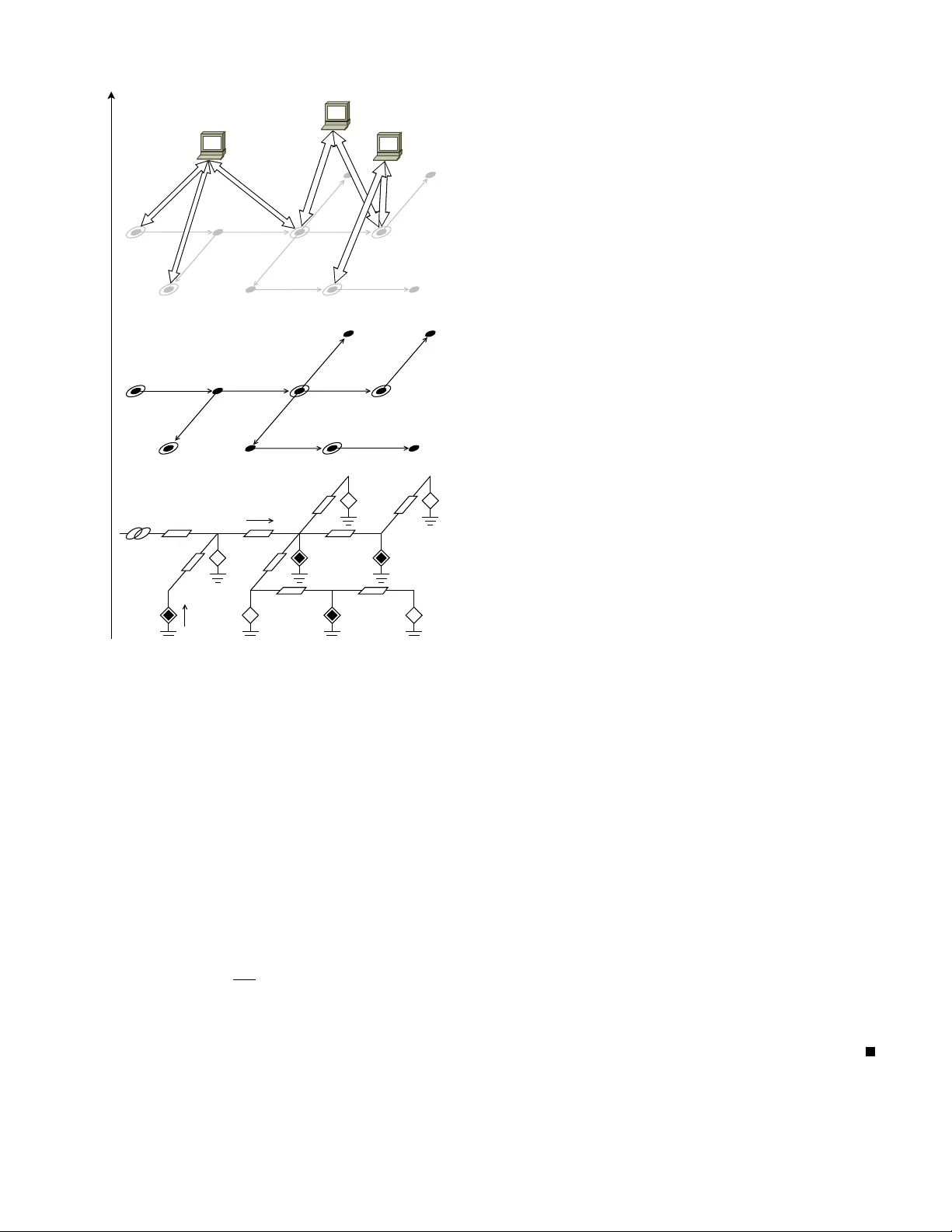
1 A distrib uted contr ol strategy f or r eactiv e power compensation in smart micr ogrids Sav erio Bolognani and Sandro Zampieri Abstract —W e consider the problem of optimal reactiv e power compensation for the minimization of power distribution losses in a smart microgrid. W e first propose an approximate model for the power distrib ution netw ork, which allows us to cast the problem into the class of con vex quadratic, linearly constrained, optimization problems. W e then consider the specific problem of commanding the microgenerators connected to the micr ogrid, in order to achieve the optimal injection of r eactive po wer . For this task, we design a randomized, gossip-lik e optimization algorithm. W e sho w how a distributed appr oach is possible, where microgenerators need to ha ve only a partial knowledge of the problem parameters and of the state, and can perform only local measurements. For the proposed algorithm, we pro vide conditions f or con v ergence together with an analytic character- ization of the conver gence speed. The analysis shows that, in radial networks, the best perf ormance can be achieved when we command cooperation among units that are neighbors in the electric topology . Numerical simulations are included to validate the proposed model and to confirm the analytic results about the performance of the proposed algorithm. I . I N T RO D U C T I O N Most of the distributed optimization methods ha ve been deriv ed for the problem of dispatching part of a large scale optimization algorithm to different processing units [1]. When the same methods are applied to networked control systems (NCS) [2], howe v er , different issues arise. The way in which decision v ariables are assigned to dif ferent agents is not part of the designer degrees of freedom. Moreo ver , each agent has a local and limited kno wledge of the problem parameters and of the system state. Finally , the information exchange between agents can occur not only via a giv en communication channel, but also via local actuation and subsequent measurement performed on an underlying physical system. The extent of these issues depends on the particular application. In this work we present a specific scenario, belonging to the motiv ating framew ork of smart electrical power distrib ution networks [3], [4], in which these features play a central role. In the last decade, power distribution networks hav e seen the introduction of distributed microgeneration of electric energy (enabled by technological advances and moti v ated by economical and en vironmental reasons). This fact, together with an increased demand and the need for higher quality of service, has been dri ving the integration of a large amount of information and communication technologies (ICT) into these networks. Among the many different aspects of this transition, we focus on the control of the distributed energy resources (DERs) inside a smart microgrid [5], [6]. A microgrid is a The authors are with the Department of Information Engineering, Uni- versity of Padov a, Italy . Mailing address: via Gradenigo 6/B, 35131 Padov a, Italy . Phone: +39 049 827 7757. Fax +39 049 827 7614. Email: { saverio.bolognani, zampi } @dei.unipd.it . portion of the lo w-v oltage po wer distribution network that is managed autonomously from the rest of the network, in order to achie ve better quality of the service, improv e efficienc y , and pursue specific economic interests. T ogether with the loads connected to the microgrid (both residential and industrial customers), we also have microgeneration devices (solar panels, combined heat-and-power plants, micro wind turbines, etc.). These devices are connected to the microgrid via electronic interfaces (in verters), whose main task is to enable the injection of the produced po wer into the microgrid. Howe v er , these de vices can also perform different other tasks, denoted as ancillary services [7], [8], [9]: reactiv e power compensation, harmonic compensation, voltage support. In this work we consider the problem of optimal r eactive power compensation . Loads belonging to the microgrid may require a sinusoidal current which is not in phase with voltage. A con venient description for this, consists in saying that they demand reacti ve power together with acti ve power , associated with out-of-phase and in-phase components of the current, respectiv ely . Reactiv e power is not a “real” physical power , meaning that there is no energy con version in volv ed nor fuel costs to produce it. Like acti ve power flows, reactive power flows contribute to power losses on the lines, cause voltage drop, and may lead to grid instability . It is therefore preferable to minimize reactiv e power flows by producing it as close as possible to the users that need it. W e explore the possibility of using the electronic interface of the microgeneration units to optimize the flo ws of reacti ve po wer in the microgrid. Indeed, the in verters of these units are generally oversized, because most of the distributed energy sources are intermittent in time, and the electronic interface is designed according to the peak power production. When they are not working at the rated power , these in verters can be commanded to inject a desired amount of reacti ve power at no cost [10]. This idea has been recently in vestigated in the literature on power systems [11], [12], [13]. Ho we ver , these works consider a centralized scenario in which the parameters of the entire power grid are kno wn, the controller can access the entire system state, the microgenerators are in small number , and they receive reacti ve power commands from a central processing unit. In [14], a hierarchical and secure architec- ture has been proposed for supporting such dispatching. The contribution of this w ork consists in casting the same problem in the frame work of networked control systems and distributed optimization. This approach allows the design of algorithms and solutions which can guarantee scalability , robustness to insertion and remov al of the units, and compliance with the actual communication capabilities of the de vices. Up to now , the fe w attempts of applying these tools to the power distribution networks ha ve focused on grids comprising a 2 large number of mechanical synchronous generators, instead of po wer in verters. See for example the stability analysis for these systems in [15] and the decentralized control synthesis in [16]. Seminal attempts to distribute optimal reactive power compensation algorithms in a large-scale po wer network, consisted in dividing the grid into separate regions, each one provided with a supervisor [17], [18]. Each of the supervisors can access all the regional measuments and data (including load demands) and can solve the corresponding small-scale optimization problem, enforcing consistency of the solution with the neighbor regions. Instead, preliminary attempts of de- signing distrib uted reacti ve power compensation strategies for microgrids populated by po wer in verters hav e been performed only very recently . Ho we ver , the a vailable results in this sense are mainly supported by heuristic approaches [19], they follow suboptimal criteria for sharing a cumulative reactive power command among microgenerators [20], and in some cases do not implement any communication or synergistic behavior of the microgenerators [21]. In [22], a multi-agent-system approach has been emplo yed for commanding reacti ve po wer injection in order to support the microgrid v oltage profile. The contribution of this paper is tw ofold. On one side, we propose a rigorous analytic deriv ation of an approximate model of the po wer flows. The proposed model can be considered as a generalization of the DC power flow model commonly adopted in the power system literature (see for example [23, Chapter 3] and references therein). V ia this model, the optimal reacti ve power flow (ORPF) problem is casted into a quadratic optimization (Section III). The second contribution is to propose and to analyze a distributed strategy for commanding the reacti ve po wer injection of each microgeneration unit, capable of optimizing reactiv e po wer flows across the microgrid (Section IV). In Section V we characterize con v ergence of the proposed algorithm to the global optimal solution, and we study its performance. In Section VI we show how the performance of this algorithm can be optimized by a proper choice of the communication strategy . In Section VII, we finally validate both the proposed model and the proposed algorithm via simulations. I I . M A T H E M A T I C A L P R E L I M I NA R I E S A N D N OTA T I O N Let G = ( V , E , σ, τ ) be a directed graph, where V is the set of nodes, E is the set of edges, and σ, τ : E → V are two functions such that edge e ∈ E goes from the source node σ ( e ) to the terminal node τ ( e ) . T wo edges e and e 0 are consecutive if { σ ( e ) , τ ( e ) } ∩ { σ ( e 0 ) , τ ( e 0 ) } is not empty . A path is a sequence of consecuti ve edges. In the rest of the paper we will often introduce complex- valued functions defined on the nodes and on the edges. These functions will also be intended as v ectors in C n (where n = |V | ) and C |E | . Gi ven a v ector u , we denote by ¯ u its (element- wise) complex conjugate, and by u T its transpose. Let moreov er A ∈ { 0 , ± 1 } |E |× n be the incidence matrix of the graph G , defined via its elements [ A ] ev =    − 1 if v = σ ( e ) 1 if v = τ ( e ) 0 otherwise. If W is a subset of nodes, we define by 1 W the column vector whose elements are [ 1 W ] v ( 1 if v ∈ W 0 otherwise . Similarly , if w is a node, we denote by 1 w the column v ector whose v alue is 1 in position w , and 0 elsewhere, and we denote by 1 the column vector of all ones. If the graph G is connected (i.e. for every pair of nodes there is a path connecting them), then 1 is the only vector in the null space ker A . An undirected graph G is a graph in which for e very edge e ∈ E , there e xists an edge e 0 ∈ E such that σ ( e 0 ) = τ ( e ) and τ ( e 0 ) = σ ( e ) . In case the graph has no multiple edges and no self loops, we can also describe the edges of an undirected graph as subsets { h 0 , h 00 } ⊆ V of cardinality 2. Similarly , we define a hyper graph H as a pair ( V , E ) in which each edge is a subset { h 0 , h 00 , . . . } of V , of arbitrary cardinality [24]. I I I . P RO B L E M F O R M U L A T I O N A. A model of a micro grid W e define a smart microgrid as a portion of the power dis- tribution network that is connected to the power transmission network in one point, and hosts a number of loads and micro power generators, as described for example in [5], [6] (see Figure 1, lo wer panel). For the purpose of this paper , we model a microgrid as a directed graph G , in which edges represent the power lines, and nodes represent both loads and generators that are connected to the microgrid (see Figure 1, middle panel). These include loads, microgenerators, and also the point of connection of the microgrid to the transmission grid (called point of common coupling, or PCC). W e limit our study to the steady state beha vior of the system, when all voltages and currents are sinusoidal signals at the same frequency . Each signal can therefore be represented via a complex number y = | y | e j ∠ y whose absolute v alue | y | corresponds to the signal root-mean-square value, and whose phase ∠ y corresponds to the phase of the signal with respect to an arbitrary global reference. In this notation, the steady state of a microgrid is described by the follo wing system v ariables (see Figure 1, lo wer panel): • u ∈ C n , where u v is the grid voltage at node v ; • i ∈ C n , where i v is the current injected by node v ; • ξ ∈ C |E | , where ξ e is the current flowing on the edge e . The following constraints are satisfied by u, i and ξ A T ξ + i = 0 , (1) Au + Z ξ = 0 , (2) where A is the incidence matrix of G , and Z = diag ( z e , e ∈ E ) is the diagonal matrix of line impedances, z e being the impedance of the microgrid power line corresponding to the edge e . Equation (1) corresponds to Kirchhoff ’ s current law (KCL) at the nodes, while (2) describes the voltage drop on the edges of the graph. Each node v of the microgrid is then characterized by a law relating its injected current i v with its voltage u v . W e model the PCC (which we assume to be node 0 ) as an ideal 3 Electric network Graph model Control u v i v ξ e z e v σ ( e ) τ ( e ) e 0 C i C j C k Figure 1. Schematic representation of the microgrid model. In the lower panel a circuit representation is given, where black diamonds are microgenerators, white diamonds are loads, and the left-most element of the circuit represents the PCC. The middle panel illustrates the adopted graph representation for the same microgrid. Circled nodes represent compensators (i.e. microgener- ators and the PCC). The upper panel shows how the compensators can be divided into ov erlapping clusters in order to implement the control algorithm proposed in Section IV. Each cluster is provided with a supervisor with some computational capability . sinusoidal voltage generator at the microgrid nominal voltage U N with arbitrary , b ut fixed, angle φ u 0 = U N e j φ . (3) W e model loads and microgenerators (that is, every node v of the microgrid e xcept the PCC) via the follo wing law relating the voltage u v and the current i v u v ¯ i v = s v     u v U N     η v , ∀ v ∈ V \{ 0 } , (4) where s v is the nominal complex power and η v is a char- acteristic parameter of the node v . The model (4) is called exponential model [25] and is widely adopted in the literature on po wer flow analysis [26]. Notice that s v is the complex power that the node would inject into the grid, if the v oltage at its point of connection were the nominal voltage U N . The quantities p v := Re( s v ) and q v := Im( s v ) are denoted as active and r eactive power , respectiv ely . The nominal complex powers s v corresponding to microgrid loads are such that { p v < 0 } , meaning that positi ve activ e power is supplied to the devices. The nominal comple x powers corresponding to microgenerators, on the other hand, are such that { p v ≥ 0 } , as positiv e acti ve power is injected into the grid. The parameter η v depends on the particular device. For example, constant power , constant current, and constant impedance de vices are described by η v = 0 , 1 , 2 , respecti vely . In this sense, this model is also a generalization of ZIP models [25], which also are very common in the power system literature. Microgenerators fit in this model with η v = 0 , as they generally are commanded via a complex po wer reference and the y can inject it independently from the voltage at their point of connection [5], [6]. The task of solving the system of nonlinear equations gi ven by (1), (2), (3), and (4) to obtain the grid voltages and currents, giv en the network parameters and the injected nominal powers { s v , v ∈ V \{ 0 }} at e very node, has been extensi vely covered in the literature under the denomination of power flow analysis (see for example [23, Chapter 3]). In the follo wing, we derive an approximate model for the microgrid state, which will be used later for the setup of the optimization problem and for the deriv ation of the proposed distributed algorithm. T o do so, a couple of technical lemmas are needed. Lemma 1. Let L be the complex valued Laplacian L := A T Z − 1 A . Ther e exists a unique symmetric matrix X ∈ C n × n such that ( X L = I − 11 T 0 X 1 0 = 0 . (5) Pr oof: Let us first prov e the e xistence of X . As k er L = span 1 = k er( I − 11 T 0 ) , there exists X 0 ∈ C n × n such that X 0 L = ( I − 11 T 0 ) . Let X = X 0 ( I − 1 0 1 T ) . Then X L = X 0 ( I − 1 0 1 T ) L = X 0 L = I − 11 T 0 , X 1 0 = X 0 ( I − 1 0 1 T ) 1 0 = 0 . Existence is then guaranteed. T o prov e uniqueness, notice that  X 1 1 T 0   L 1 0 1 T 0 0  =  X L + 11 T 0 X 1 0 1 T L 1 T 1 0  =  I 0 0 1  . Therefore  X 1 1 T 0  =  L 1 0 1 T 0 0  − 1 , and uniqueness of X follo ws from the uniqueness of the in verse. Moreover , as L = L T , we ha ve  X T 1 1 T 0  =  L 1 0 1 T 0 0  − T =  L T 1 0 1 T 0 0  − 1 =  X 1 1 T 0  and therefore X = X T . The matrix X depends only on the topology of the micro- grid po wer lines and on their impedance (compare it with the definition of Green matrix in [27]). Indeed, it can be sho wn that, for e very pair of nodes ( v, w ) , ( 1 v − 1 w ) T X ( 1 v − 1 w ) = Z eff v w , (6) 4 where Z eff v w represents the effective impedance of the po wer lines between node v and w . All the currents i and the voltages u of the microgrid are therefore determined by the equations          u = X i + U N e j φ 1 1 T i = 0 u v ¯ i v = s v     u v U N     η v , ∀ v ∈ V \{ 0 } , (7) where the first equation results from (1), (2), and (3) together with Lemma 1, while the second equation descends from (1), using the fact that A 1 = 0 in a connected graph. W e can see the currents i and the voltages u as functions i ( U N ) , u ( U N ) of U N . The following proposition provides the T aylor approximation of i ( U N ) and u ( U N ) for lar ge U N . Proposition 2. Let s be the vector of all nominal complex powers s v , including s 0 := − X v ∈V \{ 0 } s v . (8) Then for all v ∈ V we have that i v ( U N ) = e j φ  ¯ s v U N + c v ( U N ) U 2 N  u v ( U N ) = e j φ  U N + [ X ¯ s ] v U N + d v ( U N ) U 2 N  (9) for some comple x valued functions c v ( U N ) and d v ( U N ) whic h ar e O (1) as U N → ∞ , i.e. they are bounded functions for lar ge values of the nominal voltage U N . The proof of this proposition is based on elementary mul- tiv ariable analysis, b ut requires a quite inv olved notation. F or this reason it is gi ven in Appendix A. The quality of the approximation proposed in the pre vious proposition relies on having large nominal voltage U N and relativ ely small currents injected by the in verters (or supplied to the loads). This assumption is verified in practice and corresponds to correct design and operation of power distrib ution networks, where indeed the nominal voltage is chosen sufficiently large (subject to other functional constraints) in order to deliver electric power to the loads with relati vely small po wer losses on the power lines. Numerical simulation in Section VII will indeed show that the approximation is extremely good when power distribution networks are operated in their re gular regime. Remark. Notice that this appr oximation, in similar fashions, has been used in the literatur e befor e for the pr oblem of estimating power flows on the power lines (see among the others [28], [21] and r efer ences ther ein). It also shares some similarities with the DC power flow model [23, Chapter 3], extending it to the lossy case (in which lines are not pur ely inductive). The analytical rigor ous justification pr oposed her e allows us to estimate the appr oximation err or , and, mor e importantly , will pr ovide the tools to under stand what informa- tion on the system state can be gathered by pr operly sensing the micr ogrid. B. P ower losses minimization pr oblem Similarly to what has been done for example in [29], we choose activ e power losses on the po wer lines as a metric for optimality of reacti ve power flows. The total active power losses on the edges are gi ven by J tot := X e ∈E | ξ e | 2 Re( z e ) = ¯ i T Re( X ) i, (10) where we used (2) and (7), together with the properties (5) of X , to e xpress ξ as a function of i . In the scenario that we are considering, we are allowed to command only a subset C ⊂ V of the nodes of the microgrid (namely the microgenerators, also called compensators in this framew ork). W e denote by m := |C | its cardinality . Moreov er, we assume that for these compensators we are only allo wed to command the amount of reactiv e po wer q v = Im( s v ) injected into the grid, as the decision on the amount of activ e power follows imperativ e economic criteria. For example, in the case of renewable energy sources, any av ailable active power is typically injected into the grid to replace generation from traditional plants, which are more expensiv e and e xhibit a worse en vironmental impact [10]. The resulting optimization problem is then min q v , v ∈C J tot , (11) where the vector of currents i is a function of the decision variables q v , v ∈ C , via the implicit system of nonlinear equations (7). In the typical formulations of the optimal reactiv e power compensation problem, some constraints might be present. T raditional operational requirements constrain the voltage am- plitude at ev ery node to stay inside a gi ven range centered around the microgrid nominal v oltage | u v | ∈ [ U N − ∆ U, U N + ∆ U ] , v ∈ V . Moreov er , the po wer in verters that equip each microgenerator, due to thermal limits, can only provide a limited amount of reactiv e po wer . This limit depends on the size of the in verter but also on the concurrent production of acti ve power by the same device (see [21]). These constraints can be quite tight, and correspond to a set of box constr aint on the decision variables, q v ∈  q min v , q max v  , v ∈ C \{ 0 } . These constraints have been relaxed for the analysis presented in this paper , and for the subsequent design of a control strategy . This choice allo wed to conduct an analytic study of the performance of the proposed solution. One possible extension of the approach presented here, dealing ef fectiv ely with such limits, has been proposed in [30]. In the follo wing, we sho w how the approximated model proposed in the previous section can be used to tackle the optimization problem (11) and to design an algorithm for its solution. By plugging the approximate system state (9) into 5 (10), we ha ve J tot = 1 U 2 N ¯ s T Re( X ) s + 1 U 3 N ˜ J ( U N , s ) = 1 U 2 N p T Re( X ) p + 1 U 2 N q T Re( X ) q + 1 U 3 N ˜ J ( U N , s ) where p = Re( s ) , q = Im( s ) , and ˜ J ( U N , s ) := 2 Re  s T Re( X ) c ( U N )  + 1 U N ¯ c T ( U N ) Re( X ) c ( U N ) is bounded as U N tends to infinity . The term 1 U 3 N ˜ J ( U N , s ) can thus be ne glected if U N is large. Therefore, via the approximate model (9), we have been able to • approximate po wer losses as a quadratic function of the injected power; • decouple the problem of optimal power flows into the problem of optimal activ e and reacti ve po wer injection. The problem of optimal reacti ve po wer injection at the com- pensators can therefore be expressed as a quadratic, linearly constrained problem, in the form min q v ,v ∈C J ( q ) , where J ( q ) = 1 2 q T Re( X ) q , subject to 1 T q = 0 (12) where the other components of q , namely { q v , v ∈ V \C } , are the nominal amounts of reacti ve power injected by the nodes that cannot be commanded, and the constraint 1 T q = 0 directly descends from (8). The solution of the optimization problem (12) would not pose any challenge if a centralized solver knew the problem parameters X and { q v , v ∈ V \C } . These quantities depend both on the grid parameters and on the reactive power demand of all the microgrid loads. In the case of a large scale system, collecting all this information at a central location would be unpractical for many reasons, including communication constraints, delays, reduced robustness, and priv acy concerns. I V . A D I S T R I B U T E D A L G O R I T H M F O R R E AC T I V E P O W E R D I S P A T C H I N G In this section, we present an algorithm that allo ws the com- pensators to decide on the amount of reacti ve power that each of them ha ve to inject in the microgrid in order to minimize the power distribution losses. The proposed approach is based on a distributed strate gy , meaning that it can be implemented by the compensators without the supervision of any central controller . In order to design such a strategy , the optimization problem is decomposed into smaller , tractable subproblems that are assigned to small groups of compensators (possibly e ven pairs of them). W e will show that the compensators can solve their corresponding subproblems via local measurements, a local knowledge of the grid topology , and a limited data processing and communication. W e will finally show that the repeated solution of these subproblems yields the solution of the original global optimization problem. It is worth remarking that the decomposition methods pro- posed in most of the literature on distrib uted optimization, for example in [31], cannot be applied to this problem because the cost function in (12) is not separable into a sum of individual terms for each agent. Approaching the decomposition of this optimization problem via its dual formulation (as proposed in many works, including the recent [32]) is also unlikely to succeed, as the feasibility of the system state must be guaranteed at an y time during the optimization process. A. Optimization pr oblem decomposition Let the compensators be divided into ` possibly ov erlapping subsets C 1 , . . . , C ` with S ` r =1 C r = C . Nodes belonging to the same subset (or cluster ) are able to communicate each other , and they are therefore capable of coordinating their actions and sharing their measurements. Each cluster is also provided with some computational capabilities for processing the collected data. This processing is performed by a cluster supervisor , capable of collecting all the necessary data from the compensators belonging to the cluster and to return the result of the data processing to them (see Figure 1, upper panel). The cluster supervisor can possibly be one of the compensators in the cluster . An alternativ e implementation consists in providing all the compensators in the cluster with identical instances of the same instructions. In this case, after sharing the necessary data, they will perform e xactly the same data processing, and no supervising unit is needed. The proposed optimization algorithm consists of the fol- lowing repeated steps, which occur at time instants T t ∈ R , t = 0 , 1 , 2 , . . . . 1) A cluster C r ( t ) is chosen, where r ( t ) ∈ { 1 , . . . , ` } . 2) The compensators in C r ( t ) , by sharing their state (the injected reactiv e powers q k , k ∈ C r ( t ) ) and their mea- surements (the voltages u k , k ∈ C r ( t ) ), determine their new feasible state that minimizes the global cost J ( q ) , solving the optimization subpr oblem in which the nodes not belonging to C r ( t ) keep their state constant. 3) The compensators in C r ( t ) update their states q k , k ∈ C r ( t ) by injecting the new reactive powers computed in the previous step. In the follo wing, we provide the necessary tools for im- plementing these steps. In particular , we sho w how the com- pensators belonging to the cluster C r ( t ) can update their state to minimize the total power distribution losses based only on their partial kno wledge of the electrical network topology and on the measurements they can perform. Consider the optimization (12), and let us distinguish the controllable and the uncontrollable components of the v ector q . Assume with no loss of generality that the first m components of q are controllable (i.e. they describe the reactiv e power injected by the compensators) and that the remaining n − m are not controllable. The state q is thus partitioned as q =  q C q V \C  where q C ∈ R m and q V \C ∈ R n − m . According to this partition 6 of q , let us also partition the matrix Re( X ) as Re( X ) =  M N N T Q  . (13) Let us also introduce some con venient notation. Consider the subspaces S r :=    q C ∈ R m : X j ∈C r [ q C ] j = 0 , [ q C ] j = 0 ∀ j 6∈ C r    , and the m × m matrices Ω := 1 2 m X h,k ∈C ( 1 h − 1 k )( 1 h − 1 k ) T = I − 1 m 11 T , Ω r := 1 2 |C r | X h,k ∈C r ( 1 h − 1 k )( 1 h − 1 k ) T = diag( 1 C r ) − 1 |C r | 1 C r 1 T C r , where diag( 1 C r ) is the m × m diagonal matrix whose diagonal is the v ector 1 C r . Notice that S r = span Ω r . W e list some useful properties: i) Ω 2 r = Ω r and Ω ] r = Ω r , where ] means pseudoin verse. ii) The matrices Ω r , Ω r M Ω r and (Ω r M Ω r ) ] hav e entries different from zero only in position h, k with h, k ∈ C r . iii) k er(Ω r M Ω r ) ] = k er Ω r and span(Ω r M Ω r ) ] = span Ω r , and thus (Ω r M Ω r ) ] = (Ω r M Ω r ) ] Ω r . If the system is in the state q =  q C q V \C  and cluster C r is activ ated, the corresponding cluster supervisor has to solve the optimization problem q opt, r C := arg min q 0 C J  q 0 C q V \C  subject to q 0 C − q C ∈ S r . (14) Using the standard formulas for quadratic optimization it can be shown that q opt, r C = q C − (Ω r M Ω r ) ] ∇ J, (15) where ∇ J = M q C + N q V \C (16) is the gradient of J  q C q V \C  with respect to the decision variables q C . Notice that, by using property ii) of the matrices (Ω r M Ω r ) ] , we have  q opt, r C  h = ( q h − P k ∈C r h (Ω r M Ω r ) ] i hk [ ∇ J ] k if h ∈ C r q h if h / ∈ C r . (17) In the following, we show how the supervisor of C r can perform an approximate computation of  q opt, r C  h , h ∈ C r , based on the information a vailable within C r . B. Hessian reconstruction fr om local topology information Compensators belonging to the cluster C r can infer some information about the Hessian M . More precisely they can determine the elements of the matrix (Ω r M Ω r ) ] appearing in (17). Define R eff as a m × m matrix with entry in h, k ∈ C equal to Re  Z eff hk  , where Z eff hk are the mutual effecti ve impedances between pairs compensators h, k . From (6) and (13) we ha ve that [ R eff ] hk = Re  Z eff hk  = ( 1 h − 1 k ) T M ( 1 h − 1 k ) (18) and so we can write R eff = X h,k ∈C 1 h ( 1 h − 1 k ) T M ( 1 h − 1 k ) 1 T k = diag( M ) 11 T + 11 T diag( M ) − 2 M where diag( M ) is the m × m diagonal matrix having the same diagonal elements of M . Consequently , since Ω r 1 = 0 , we have that Ω r R eff Ω r = − 2Ω r M Ω r and then Ω r M Ω r = − 1 2 Ω r R eff Ω r . (19) Because of the specific sparseness of the matrices Ω r and via (18), we can then argue that the elements of the matrix Ω r M Ω r can be computed by the supervisor of cluster C r from the mutual effecti ve impedances Z eff hk for h, k ∈ C r . These impedances are assumed to be known by the cluster supervisor . This is a reasonable hypothesis, since the mutual effecti ve impedances can be obtained via online estimation procedures as in [33] or via ranging technologies ov er power line communications as suggested in [34]. Moreov er , in the common case in which the low-v oltage po wer distribution grid is radial, the mutual effecti ve impedances Z eff hk correspond to the impedance of the only electric path connecting node h to node k , and can therefore be inferred from a priori knowledge of the local microgrid topology . Then the cluster supervisor needs to compute the pseudo- in verse of Ω r M Ω r . Notice that all these operations have to be e xecuted offline once, as these coef ficients depend only on the grid topology and impedances, and thus are not subject to change. C. Gradient estimation via local voltage measur ement Assume that nodes in C r can measure the grid voltage u k , k ∈ C r , at their point of connection. In practice, this can be done via phasor measur ement units that return both the amplitudes | u k | and phases ∠ u k of the measured voltages (see [35], [36]). Let us moreo ver assume the following. Assumption 3. All power lines in the micr ogrid have the same inductance/r esistance ratio, i.e. Z = e j θ Z wher e Z is a diagonal r eal-valued matrix, whose elements are [ Z ] ee = | z e | . Consequently , L = e − j θ A T Z − 1 A , and X := e − j θ X is a r eal-valued matrix. This assumption seems reasonable in most practical cases (see for example the IEEE standard testbeds [37]). The effects of this approximation will be commented in Section VII. 7 Similarly to the definition of q C , we define by u C the vector in C m containing the components u k with k ∈ C , i.e. the voltages that can be measured by the compensators. Consider now the maps K r : C m → C m , r = 1 , . . . , ` , defined component-wise as follo ws [ K r ( u C )] k := ( 1 |C r | P v ∈C r | u v || u k | sin( ∠ u v − ∠ u k − θ ) if k ∈ C r 0 if k 6∈ C r . (20) Notice first that K r ( u C ) can be computed locally by the supervisor of the cluster r , from the v oltage measurements of the compensators belonging to C r . The following result shows how the function K r ( u C ) is related with the gradient of the cost function, introduced in (16). Proposition 4. Let K r ( u C ) be defined as in (20) . Then the elements [ ∇ J ] k , k ∈ C r , of the gradient intr oduced in (16) can be decomposed as [ ∇ J ] k = cos θ [ K r ( u C )] k + α r + 1 U N h ˜ K r ( u C ) i k , (21) wher e h ˜ K r ( u C ) i k is bounded as U N → ∞ , and α r is a constant independent of the compensator inde x k . Pr oof: It can be seen that, for k ∈ C r , [ K r ( u C )] k = − Im  e − j θ 1 |C r |  1 T C r ¯ u  u k  . By using (9), and via a series of simple but rather tedious computation it can be seen that (21) holds with α r = cos θ |C r | Im  e − j 2 θ  1 T C r X s  + cos θ |C r | U N Im  e − j θ  1 T C r ¯ d  − sin θ cos θ U 2 N and h ˜ K r ( u C ) i k = cos θ Im  e − j θ d k  + cos θ U N |C r | Im  e − j θ  1 T C r X s  [ X ¯ s ] k  + cos θ U 2 N |C r | Im  e − j 2 θ  1 T C r X s  d k  + cos θ U 2 N |C r | Im  1 T C r ¯ d  [ X ¯ s ] k  + cos θ U 3 N |C r | Im  e − j θ  1 T C r ¯ d  d k  , which according to Proposition 2 is bounded when U N → ∞ . D. Description of the algorithm By applying Proposition 4 to expression (17) for q opt, r C we obtain that, for h ∈ C r ,  q opt, r C  h = q h − cos θ X k ∈C r h (Ω r M Ω r ) ] i hk [ K r ( u C )] k − cos θ U N X k ∈C r h (Ω r M Ω r ) ] i hk h ˜ K r ( u C ) i k , (22) where the term α r is canceled because of the specific k ernel of (Ω r M Ω r ) ] . Because 1 U N ˜ K r is infinitesimal as U N → ∞ , then equation (22), together with identity (19), suggests the following approximation for q opt, r C  [ q opt, r C  h = q h + 2 cos θ X k ∈C r h  Ω r R eff Ω r  ] i hk [ K r ( u C )] k (23) which can be computed for all h ∈ C r by the supervi- sor of cluster r from local information, namely the local network electric properties and the voltage measurements at the compensators belonging to C r . Notice also that, as span(Ω r R eff Ω r ) ] = span Ω r , we have that P h  q opt, r C  h − q h = 0 , and therefore the constraint 1 T q = 0 remains satisfied. Based on this result, we propose the following iterati ve algorithm, whose online part is also depicted in Figure 2 in its block diagram representation. O FFL I N E P RO C E D U R E • The supervisor of each cluster C r gathers the system parameter [ R eff ] hk , h, k ∈ C r ; • each supervisor computes the elements h  Ω r R eff Ω r  ] i hk , h, k ∈ C r . O N L I N E P R OC E D U R E At each iteration t : • a cluster C r is randomly selected among all the clusters; • each compensator h ∈ C r measures its v oltage u h ; • each compensator h ∈ C r sends its voltage u h and its state q h (the amount of reacti ve po wer they are injecting into the grid) to the cluster supervisor; • the cluster supervisor computes K r ( u C ) , via (20); • the cluster supervisor computes  [ q opt, r C  h for all h ∈ C r via (23); • each compensator h ∈ C r receiv es the value  [ q opt, r C  h from the cluster supervisor and updates its injection of reactiv e po wer into the grid (i.e. q h ) to that value. Remark. One possible way of randomly selecting one cluster C r at each iteration, is the following. Let each cluster su- pervisor be pr ovided with a timer , each one governed by an independent P oisson pr ocess, which trig gers the cluster after exponentially distributed waiting times. If the time requir ed for the execution of the algorithm is ne gligible with r espect to the typical waiting time of the P oisson pr ocesses, this strate gy allows to construct the sequence of independent symbols r ( t ) , t = 0 , 1 , 2 , . . . , in a pur ely decentralized way (see for example [38]). Remark. It is important to notice that the distrib uted imple- mentation of the algorithm is only possible because of the specific physical system that we ar e considering. By sensing the system locally , nodes can infer some global information on the system state (namely , the gradient of the cost function) that otherwise would depend on the states of all other nodes. F or this r eason, it is necessary that, after each iteration of the algorithm, the micr ogenerator s actuate the system 8 Power distribution network q C u C q V \C p 2 cos θ (Ω r R eff Ω r ) ♯ u V \C K r ( u C ) 1 z − 1 Discrete time integrator Figure 2. Block diagram representation of the proposed distributed algorithm. The repeated solution of different optimization subproblems corresponds to a switching discrete time feedback system. Double arro ws represent vector signals. The power distrib ution network block receiv es, as inputs, the activ e and reactive power injection of both compensators (nodes in C ) and loads (nodes in V \C ). It gives, as outputs, the voltages at the nodes. The voltages at the compensators ( u C ) can be measured, and provide the feedback signal for the control laws. Notice that the control law corresponding to a specific cluster r requires only the voltage measurements performed by the compensators belonging to the cluster ( u k , k ∈ C r ), and it updates only the reactiv e power injected by the same compensators ( q k , k ∈ C r ), while the other compensators hold their reactive power injection constant. implementing the optimization step, so that subsequent mea- sur ement will r eflect the state c hange. This appr oach r esembles some other applications of distributed optimization, e.g . the radio transmission power contr ol in wir eless networks [39] and the traf fic congestion pr otocol for wired data networks [40], [41]. Also in these cases, the iterative tuning of the decision variables (radio power , transmission rate) depends on congestion feedback signals that ar e function of the entir e state of the system. However , these signals can be detected locally by each a gent by measuring err or rates, signal-to-noise ratios, or specific feedbac k signals in the pr otocol. V . C O N V E R G E N C E O F T H E A L G O R I T H M In this section we will gi ve the conditions ensuring that the proposed iterative algorithm conv erges to the optimal solution, and we will analyze its con vergence rate. In fact, according to (23), the dynamics of the algorithm is described by the iteration q C ( t + 1) = q C ( t ) − cos θ (Ω r ( t ) M Ω r ( t ) ) ] K r ( t ) ( u C ( t )) . (24) where the voltages u C ( t ) are a function of the reactive power q C ( t ) , q V \C and of the activ e power p . W e will consider instead the iteration q C ( t + 1) = q C ( t ) −  Ω r ( t ) M Ω r ( t )  ] ( M q C ( t ) + N q V \C ) , (25) which descends from (15) and which differs from (24) for the term cos θ U N  Ω r ( t ) M Ω r ( t )  ] ˜ K r ( t ) ( u C ) , as one can verify by inspecting (22). This difference is infinitesimal as U N → ∞ . Therefore in the sequel we will study the con vergence of (25), while numerical simulations in Section VII will support the proposed approximation, showing how both the algorithm steady state performance and the rate of con vergence are practically the same for the exact system and the approximated model. Remark. A formal pr oof of the con verg ence of the discrete time system (24) could be done based of the mathematical tools pr oposed in Sections 9 and 10 of [42] dedicated to the stability of perturbed systems. However , in our setup there ar e a number of complications that make the application of those techniques not easy . The first is that, since u C ( t ) is r elated to q C ( t ) in an implicit way , then (24) is in fact a nonlinear implicit (also called descriptor) system with state q C ( t ) . The second dif ficulty comes fr om the fact that (24) is a nonlinear randomly time-varying (also called switching) system. In order to study the system (25), we introduce the auxiliary variable x = q C − q opt C ∈ R m , where q opt is the solution of the optimization problem (12), and q opt C are the elements of q opt corresponding to the nodes in C . In this notation, it is possible to explicitly e xpress the iteration (25) as a discrete time system in the form x ( t + 1) = F r ( t ) x ( t ) , x (0) ∈ k er 1 T , (26) where F r = I − (Ω r M Ω r ) ] M . (27) The matrices F r hav e some nice properties which are listed below . i) The matrices F r are self-adjoint matrices with respect to the inner product h· , ·i M , defined as h x, y i M := x T M y . Therefore F T r M = M F r , and thus they have real eigen- values. ii) The matrices F r are projection operators, i.e. F 2 r = F r , and they are orthogonal projections with respect to the inner product h· , ·i M , i.e. h F r x, F r x − x i M = x T F T r M ( F r x − x ) = 0 . Notice that, as span(Ω r M Ω r ) ] = span Ω r , ker 1 T is a positiv ely in variant set for (26), namely F r (k er 1 T ) ⊆ k er 1 T for all r . It is clear that q ( t ) conv erges to the optimal solution q opt if and only if x ( t ) con verges to zero for any initial condition x (0) ∈ k er 1 T . A necessary condition for this to happen is that there are no nonzero equilibria in the discrete time system (26), namely that the only x ∈ k er 1 T such that F r x = x for all r must be x = 0 . The following proposition provides a con venient character- ization of this property , in the form of a connectivity test. Let H be the hypergraph whose nodes are the compensators, and 9 whose edges are the clusters C r , r = 1 , . . . , ` . This hypergraph describes the communication network needed for implement- ing the algorithm: compensators belonging to the same edge (i.e. cluster) must be able to share their measurements with a supervisor and recei ve commands from it. Proposition 5. Consider the matrices F r , r = 1 , . . . , ` , defined in (27) . The point x = 0 is the only point in ker 1 T such that F r x = x for all r if and only if the hyper graph H is connected. Pr oof: The proposition is part of the statement of Lemma 15 in the Appendix B. In order to prove that the connectivity of the hypergraph H is not only a necessary but also a suf ficient condition for the conv ergence of the algorithm, we introduce the following assumption on the sequence r ( t ) . Assumption 6. The sequence r ( t ) is a sequence of indepen- dently , identically distributed symbols in { 1 , . . . , ` } , with non- zer o pr obabilities { ρ r > 0 , r = 1 , . . . , ` } . Let v ( t ) := E  x T ( t ) M x ( t ))  = E [ J ( q ( t )) − J ( q opt )] and consider the follo wing performance metric R = sup x (0) ∈ ker 1 T lim sup { v ( t ) } 1 /t (28) which describes the exponential rate of con vergence to zero of v ( t ) . It is clear that R < 1 implies the exponential mean square conv ergence of q C ( t ) to the optimal solution q opt C . Using (26), we hav e v ( t ) = E  x ( t ) T M x ( t )  = E  x ( t ) T Ω M Ω x ( t )  = E h x ( t − 1) T F T r ( t − 1) Ω M Ω F r ( t − 1) x ( t − 1) i = x (0) T E h F T r (0) · · · F T r ( t – 1) Ω M Ω F r ( t – 1) · · · F r (0) i x (0) . Let us then define ∆( t ) = E h F T r (0) · · · F T r ( t − 1) Ω M Ω F r ( t − 1) · · · F r (0) i . V ia Assumption 6, we can argue that ∆( t ) satisfies the following linear recursiv e equation ( ∆( t + 1) = L (∆( t )) ∆(0) = Ω M Ω , (29) where L (∆) := E  F T r ∆ F r  . Moreover we ha ve that v ( t ) = x (0) T ∆( t ) x (0) . (30) Equations (29) and (30) can be seen as a discrete time linear system with state ∆( t ) and output v ( t ) . Remark. The discr ete time linear system (29) can be equiv- alently be described by the equation v ec (∆( t + 1)) = F v ec (∆( t )) , wher e vec( · ) stands for the operation of vectorization and wher e F := E  F T r ⊗ F T r  ∈ R m 2 × m 2 . Notice that F is self-adjoint with respect to the inner prod- uct h· , ·i M − 1 ⊗ M − 1 and so F , and consequently L , has real eigen values. Studying the rate R (which can be proved to be the slowest reachable and observable mode of the system (29) with the output (30), see [43]) is in general not simple. It has been done analytically and numerically for some special graph structures in [43]. It is con venient to analyze its behavior indirectly , through another parameter which is easier to compute and to study , as the follo wing result shows. Theorem 7. Assume that Assumption 6 holds true and that the hyper graph H is connected. Then the rate of con verg ence R , defined in (28) , satisfy R ≤ β < 1 , wher e β = max {| λ | | λ ∈ λ ( F ave ) , λ 6 = 1 } , with F ave := E [ F r ] . Pr oof: The proof of Theorem 7 is gi ven in the Ap- pendix B. The following result descends directly from it. Corollary 8. Assume that Assumption 6 holds true and that the hypergr aph H is connected. Then the state of the iterative algorithm described in Section IV -A con ver ges in mean squar e to the global optimal solution. Remark. Observe that, by standar d arguments based on Bor el Cantelli lemma, the exponential con ver gence in mean square implies also almost sur e conver gence to the optimal solution. The tightness of β as a bound for R has been studied in [43], by e valuating both β and R analytically and numerically for some special graph topologies. In the following we consider β as a reliable metric for the ev aluation of the algorithm performances. The following result sho ws what is the best performance (according to the bound β on the con vergence rate R ) that the proposed algorithm can achiev e. Theorem 9. Consider the algorithm (25) , and assume that H describing the clusters C r is an arbitrary connected hy- per graph defined over the nodes C . Let Assumption 6 hold. Then β ≥ 1 −  P ` r =1 ρ r |C r |  − 1 m − 1 . (31) In case all the sets C r have the same car dinality c , namely |C r | = c for all r , then β ≥ 1 − c − 1 m − 1 . (32) Pr oof: Let E r := (Ω r M Ω r ) ] M (33) E ave := E [ E r ] = ` X r =1 ρ r E r (34) 10 It is clear that β = 1 − β 0 , where β 0 = min {| λ | | λ ∈ λ ( E ave ) , λ 6 = 0 } . W e ha ve that X λ j ∈ λ ( E ave ) λ j = T r( E ave ) = T r ` X r =1 ρ r E r ! = ` X r =1 ρ r T r ( E r ) . Notice now that E r hav e eigen values zero or one and so T r ( E r ) = rank E r = dim (span E r ) = dim  span(Ω r M Ω r ) ]  = dim (span Ω r ) = |C r | − 1 . This implies that X λ j ∈ λ ( E ave ) λ j = ` X r =1 ρ r |C r | ! − 1 , and so β 0 = min {| λ | | λ ∈ λ ( E ave ) , λ 6 = 0 } ≤ P λ j ∈ λ ( E ave ) λ j m − 1 =  P ` r =1 ρ r |C r |  − 1 m − 1 . V I . O P T I M A L C O M M U N I C A T I O N H Y P E R G R A P H F O R A R A D I A L D I S T R I B U T I O N N E T W O R K In this section we present a special case in which the optimal con vergence rate of Theorem 9 is indeed achie ved via a specific choice of the clusters C r . T o obtain this result we need to introduce the following assumption, which is commonly verified in many practical cases (including the vast majority of power distribution networks and the standard IEEE testbeds [37]). Assumption 10. The distribution network is radial, i.e. the corr esponding graph G is a tree . W e start by providing some useful properties of the matrices E r . Lemma 11. The following pr operties hold true: i) span E r = span Ω r ; ii) E 2 r = E r ; iii) E r x = x for all x ∈ span Ω r . Pr oof: i) First observe that, since M is in vertible, then span E r = span(Ω r M Ω r ) ] M = span(Ω r M Ω r ) ] . Finally from the properties of the matrices (Ω r M Ω r ) ] , we obtain that span E r = span Ω r . ii) First observe that E 2 r = ( I − F r ) 2 = I − 2 F r + F 2 r . Now , since F 2 r = F r we obtain that I − 2 F r + F 2 r = I − F r = E r . iii) Let x ∈ span Ω r = span E r . Then x = E r z for some vector z and so E r x = E 2 r z = E r z = x . Let us now consider for an y pair of nodes h, k the shortest path P hk ⊆ E (where, we recall, a path is a sequence of consecutiv e edges) connecting h, k . Define moreo ver P C r := [ h,k ∈C r P hk . Lemma 12. Let Assumption 10 hold true. Then i) ( 1 h − 1 k ) T M ( 1 h 0 − 1 k 0 ) = P e ∈P hk ∩P h 0 k 0 Re( z e ) . ii) E r ( 1 h − 1 k ) = 0 if P C r ∩ P hk = ∅ . Pr oof: i) Observe that ( 1 h − 1 k ) T M ( 1 h 0 − 1 k 0 ) = ( 1 h − 1 k ) T X ( 1 h 0 − 1 k 0 ) , where with some abuse of notation we have denoted with the same symbol 1 h the vector in R m and the corresponding vector in R n . Notice that, if we hav e a current r = 1 h 0 − 1 k 0 in the network, then according to (7) we get a voltage vector u = X i + 1 U N = X ( 1 h 0 − 1 k 0 ) + 1 U N and so ( 1 h − 1 k ) T X ( 1 h 0 − 1 k 0 ) = u h − u k . Observing the following figure h 0 k 0 k h h 00 k 00 we can argue that u h − u k = u h 00 − u k 00 = P e ∈P h 00 k 00 z e and so ( 1 h − 1 k ) T M ( 1 h 0 − 1 k 0 ) = P e ∈P h 00 k 00 Re( z e ) . ii) If P C r ∩ P hk = ∅ , then Ω r M ( 1 h − 1 k ) = 1 2 |C r | X h 0 ,k 0 ∈C r ( 1 h 0 − 1 k 0 )( 1 h 0 − 1 k 0 ) T M ( 1 h 0 − 1 k 0 ) = 0 since P hk ∩ P h 0 k 0 = ∅ for all h 0 , k 0 ∈ C r . Thus E r ( 1 h − 1 k ) = (Ω r M Ω r ) ] Ω r M ( 1 h − 1 k ) = 0 . W e gi ve no w the k ey definition to characterize, together with connectivity , the optimality of the communication hypergraph H . Definition 13. The hyperedg es {C r , r = 1 , . . . , ` } of the hyper graph H ar e edge-disjoint 1 if for any r , r 0 such that r 6 = r 0 , we have that P C r ∩ P C r 0 = ∅ . In order to prov e the optimality of having edge-disjoint clusters, we need the follo wing lemma. Lemma 14. Assume that Assumptions 10 holds true and that the clusters C r ar e edge-disjoint. Then E r E r 0 = 0 for all r 6 = r 0 . 1 This definition of edge-disjoint for this specific scenario resembles a similar concept for routing problems in data networks, as for example [44]. 11 PCC Figure 3. Schematic representation of the IEEE37 testbed. Circled nodes represent microgenerators taking part to the distrib uted reactive po wer com- pensation. The thick curved lines represent clusters of size c = 2 (i.e. edges of H ) connecting pair of compensators that can communicate and coordinate their behavior . Pr oof: Let x be any vector in R m . Notice that, since span E r 0 = span Ω r 0 , then there exists z ∈ R m such that E r E r 0 x = E r Ω r 0 z = 1 2 |C r | X h,k ∈C r 0 E r ( 1 h − 1 k )( 1 h − 1 k ) T z = 0 where the last equality follows from the fact that P C r ∩ P hk = ∅ for all h, k ∈ C r 0 . From the previous lemma we can ar gue that every vector in span Ω r is eigen vector of E ave = P ` r =1 ρ r E r associated with the eigenv alue ρ r . On the other hand, recall that the hyper- graph connectivity implies that ker 1 T = P ` r =1 span Ω r = P ` r =1 span E r and hence we hav e that, besides the zero eigen value, the eigen values of E ave are exactly ρ 1 , . . . , ρ ` and so β = 1 − min r =1 ,...,` { ρ r } . The bound β is minimized by taking ρ r = 1 /` for all r , obtaining β = 1 − 1 ` . Notice finally that E r E r 0 = 0 for all r 6 = r 0 implies that P ` r =1 span E r is a direct sum and then m − 1 = ` X r =1 dim span E r = ` X r =1 ( |C r | − 1) = ` X r =1 |C r | − `. If all the sets C r hav e the same cardinality c , then `c = m + ` − 1 , and so β = 1 − 1 ` = 1 − c − 1 m − 1 which, according to Theorem 9, shows the optimality of the hypergraph. V I I . S I M U L A T I O N S In this section we present numerical simulations to v alidate both the model presented in Section III, and the randomized algorithm proposed in Section IV. T o do so, we considered a 4.8 kV testbed inspired from the standard testbed IEEE 37 [37], which is an actual portion of power distribution network located in California. W e ho wever assumed that load are balanced, and therefore all currents and voltages can be described in a single-phase phasorial notation. As shown in Figure 3, some of the nodes are microgen- erators and are capable of injecting a commanded amount of reactive power . Notice that the PCC (node 0 ) belongs to the set of compensators. This means that the microgrid is allowed to change the amount of reactiv e power gathered from the transmission grid, if this reduces the power distrib ution losses. The nodes which are not compensators, are a blend of constant-power , constant-current, and constant-impedance loads, with a total power demand of almost 2 MW of active power and 1 MV AR of reacti ve power (see [37] for the testbed data). The network topology is radial. While this is not a necessary condition for the algorithm, this is typical in basically all power distrib ution netw orks. Moreover , the choice of a radial grid allows the v alidation of the optimality result of Section VI for the clustering of the compensators. The length of the power lines range from a minimum of 25 meters to a maximum of almost 600 meters. The impedance of the power lines differs from edge to edge (for example, resistance ranges from 0.182 Ω /km to 1.305 Ω /km). Howe ver , the inductance/resistance ratio e xhibits a smaller variation, ranging from ∠ z e = 0 . 47 to ∠ z e = 0 . 59 . This justifies Assumption 3, in which we claimed that ∠ z e can be considered constant across the network. The ef fects of this approximation will be commented later . W ithout any distributed reacti ve po wer compensation, distri- bution power losses amount to 61.6 kW , 3.11% of the deliv ered activ e po wer . Giv en this setup, we first estimate the quality of the linear approximated model proposed in Section III. As shown in Figure 4, the approximation error results to be negligible. W e then simulated the behavior of the algorithm proposed in Section IV. W e considered the two following clustering choices: • edge-disjoint gossip: motiv ated by the result stated in Section VI, we enabled pairwise communication between compensator in a way that guarantees that the clusters (pairs) are edge-disjoint; the resulting hyper graph H is represented as a thick line in Figure 3; • star topology: clusters are in the form C r = { 0 , v } for all v ∈ C \{ 0 } ; the reason of this choice is that, as 0 is the PCC, the constraint 1 T q = 0 is inherently satisfied: whate ver v ariation in the injected reacti ve po wer is applied by v , it is automatically compensated by a variation in the demand of reacti ve po wer from the transmission grid via the PCC. In Figure 5 we plotted the result of a single execution of the algorithm in the edge-disjoint gossip case. One can see that the 12 1 36 4 , 500 4 , 600 4 , 700 4 , 800 node v | u v | [V] 1 36 − 3 · 10 − 3 − 2 · 10 − 3 − 1 · 10 − 3 0 node v ∠ u v [rad] Figure 4. Comparison between the network state (node voltages) computed via the exact model induced by (1), (2), (4), and (3) ( ◦ ), and the approximate model proposed in Proposition 2 ( + ). 0 5 10 15 20 25 30 50 , 000 55 , 000 60 , 000 iteration losses [W] Figure 5. Po wer distribution losses resulting by the execution of the proposed algorithm. A edge-disjoint hypergraph, yielding optimal con vergence speed, has been adopted. The dashed line represent the minimum losses that can be achiev ed via centralized numerical optimization. algorithm con verges quite f ast, reducing losses to a minimum that is extremely close to the best achiev able solution. The results achieved by the proposed algorithm on this testbed are summarized in the following table. Losses before optimization 61589 W Fraction of deli vered po wer 3.11 % Losses after optimization 50338 W Fraction of deli vered po wer 2.55 % losses reduction 18.27 % Minimum losses J opt 50253 W Fraction of deli vered po wer 2.54 % losses reduction 18.41 % The minimum losses J opt is the solution of the original optimization problem (11), has been obtained by a centralized numerical solver , and represent the minimum losses that can be achieved by properly choosing the amount of reactiv e power injected by the compensators (and retrieved from the PCC). The dif ference between this minimum and the minimum achiev ed by the algorithm proposed in this paper is partly due to the approximation that we introduced when we modeled the microgrid (assuming large nominal voltage U N ), and partly due to the assumption that θ is constant across the network. Further simulati ve in vestigation on this testbed sho wed that the effect of this last assumption is largely predominant, compared to the ef fects of the approximation in the microgrid state equations. Still, the combined ef fect of these two terms is minimal, in practice. In Figure 6 we compared the behavior of the two considered clustering strategies. One can notice different things. First, both strategies con verge to the same minimum, which is slightly larger than the minimum losses that could be achieved by solving the original, nonconv ex optimization problem. As expected, the clustering choice do not affect the steady state performance of the algorithm. Second, the performance of the edge-disjoint gossip algorithm results indeed to be better than the star topology in the long-time regime, as the analysis in Section VI suggests, and its slope corresponds to the fastest achiev able rate of con vergence, as predicted by Theorem 9. Third, one can see that, while the performance metric that we adopted is meaningful for describing the long-time re gime, it does not describe, in general, the initial stage (or short-time behavior). Indeed, in the initial transient, the full dynamics of the system (25) contribute to the algorithm behavior . This is evident in the star-topology strategy . In the edge-disjoint case, on the other hand, all the eigen values of the systems (25) result to be the same, and thus the adopted performance metric (the slowest eigenv alue) fully describes the algorithm ev olution. This fact suggests that a different metric can possibly be adopted, in order to better characterize the two regimes. Choosing the most appropriate metric requires a preliminary deriv ation of a dynamic model for the variation of reactive power demands of the loads in time. In the case of time- varying loads, different strategies will corresponds to different steady-state behaviors of the algorithm. W e expect that an L 2 − type metric will be needed for the characterization of the performance of dif ferent clustering choices, while the slo west eigen value will not be informative enough in this sense. A preliminary study in this sense has been proposed in [45]. V I I I . C O N C L U S I O N S The proposed model for the problem of optimal reactive power compensation in smart microgrids exhibits two main features. First, it can be casted into the framework of quadratic optimization, for which robust solvers are av ailable and the performance analysis becomes tractable; second, it shows how the physics of the system can be exploited to design a distributed algorithm for the problem. On the basis of the proposed model, we have been able to design a distributed, leaderless and randomized algorithm for the solution of the optimization problem, requiring only local communication and local knowledge of the network topology . W e then proposed a metric for the performance of the algorithm, for which we are able to provide a bound on the best achiev able performances. W e are also able to tell which clustering choice is capable of gi ving the optimal performances. It is interesting that the optimal strate gy requires 13 0 10 20 30 40 50 60 70 100 1 , 000 10 , 000 iteration E [ J ( q ( t )) − J opt ] [W] Figure 6. Simulation of the expected behavior of the algorithm for different clustering strategies. The dif ference between power losses at each iteration of the algorithm (averaged over 1000 realizations) and the minimum possible losses J opt , has been plotted for two different clustering choices: edge-disjoint gossip (solid line) and star topology (dashed). The slope represented via a dotted line represent the best possible rate of conv ergence that the algorithm can achie ve, according to Theorem 9. short-range communications: this is a notable consequence of the presence of an underlying physical system, considered that consensus algorithm (which share many features with the proposed algorithm) benefit from long-range communication that shorten the graph diameter . At the same time, this result is also motiv ating from the technological point of view , because achieving cooperation of in verters that are far apart in the microgrid presents a number of issues (e.g. time synchronization, limited range of power line communication technologies). Motiv ated by the final remarks of Section VII, we plan to add two elements to the picture in the next future: the network dynamics (both the dynamic behavior of the po wer demands, and the electrical response of the system when actuated), and the presence of operational constraints for the compensators, whose capability of injecting reactiv e po wer is limited and possibly time v arying. A P P E N D I X A P RO O F O F P RO P O S I T I O N 2 W e first introduce the new variable  := 1 /U N . W e also assume, with no loss of generality , that the phase of the voltage at the PCC is φ = 0 . This way we can see the currents i and the v oltages u as functions i (  ) , u (  ) of  , determined by the equations      u = X i +  − 1 1 1 T i = 0 u v ¯ i v = s v | u v | η v , ∀ v ∈ V \{ 0 } (35) W e construct the T aylor approximation of u (  ) and i (  ) around  = 0 . Let us define δ v (  ) := i v (  )  − 1 − ¯ s v λ v (  ) := u v (  )  − 1 −  − 2 − [ X ¯ s ] v (36) and substitute them into (35). W e get a system of equations in δ, λ,  which can be written as ( G v ( δ, λ,  ) = 0 , ∀ v ∈ V F v ( δ, λ,  ) = 0 , ∀ v ∈ V where G 0 ( δ, λ,  ) := λ 0 F 0 ( δ, λ,  ) := X w ∈V δ w and, for all v 6 = 0 , G v ( δ, λ,  ) := λ v − X w ∈V [ X ] v w δ w , F v ( δ, λ,  ) := 1 +  2 λ v +  2 X w ∈V [ X ] v w ¯ s w ! ( s v + ¯ δ v ) − s v      1 +  2 λ v +  2 X w ∈V [ X ] v w ¯ s w      η v . W e have 2 n complex equations in 2 n + 1 complex variables. W e interpret now the complex numbers as vectors in R 2 and G v , F v as functions from R 2 n × R 2 n × R 2 to R 2 . Observe that G v ( δ, λ,  ) | δ =0 ,λ =0 , =0 = 0 and F v ( δ, λ,  ) | δ =0 ,λ =0 , =0 = 0 for all v ∈ V . By the implicit function theorem, if the matrix        ∂ G v ∂ δ w  v ,w ∈V  ∂ G v ∂ λ w  v ,w ∈V  ∂ F v ∂ δ w  v ,w ∈V  ∂ F v ∂ λ w  v ,w ∈V       ev aluated in δ = 0 , λ = 0 ,  = 0 is inv ertible, then δ (  ) , λ (  ) hav e continuous deriv atives in  = 0 . In order to determine this matrix we need to introduce the following notation. If a ∈ C , and a = a R + j a I with a R , a I ∈ R , then we define h a i :=  a R − a I a I a R  W ith this notation observe that, if a, x ∈ C and we consider those complex numbers as vectors in R 2 and if we consider the function f ( x ) := ax as a function from R 2 to R 2 , then we hav e that ∂ f /∂ x = h a i . Notice moreover that the the function g ( x ) := ¯ x has ∂ g ∂ x = N :=  1 0 0 − 1  From these observ ations we can ar gue that ∂ G 0 ∂ δ w = 0 , ∂ G 0 ∂ λ w = ( I if w = 0 0 if w 6 = 0 ∂ F 0 ∂ δ w = I , ∂ F 0 ∂ λ w = 0 Instead for all v 6 = 0 we ha ve that ∂ G v ∂ λ w = ( I if w = v 0 if w 6 = v 14 while ∂ G v ∂ δ w = h− X v w i ∀ w ∈ V . Observe finally that, if w 6 = v , then ∂ F v /∂ λ w = ∂ F v /∂ δ w = 0 and that ∂ F v ∂ δ v = * 1 +  2 λ v +  2 X w ∈V [ X ] v w ¯ s w + N which ev aluated in  = 0 yields the matrix N . On the other hand, ∂ F v ∂ λ v = h  2 ( s v + ¯ δ v ) i − s v ∂   1 +  2 λ v +  2 P w ∈V [ X ] v w ¯ s w   η v ∂ λ v where s v is a 2 -dimensional column vector and ∂ | 1+ λ v | η v ∂ λ v is a 2 -dimensional ro w vector . With some easy computations it can be seen that ∂ | 1+ λ v | η v ∂ λ v , ev aluated in  = 0 , yields [0 0] . Hence in  = 0 we hav e ∂ F v ∂ λ v = h 0 i . W e can conclude that for δ = 0 , λ = 0 ,  = 0 we ha ve        ∂ G v ∂ δ w  v ,w ∈V  ∂ G v ∂ λ w  v ,w ∈V  ∂ F v ∂ δ w  v ,w ∈V  ∂ F v ∂ λ w  v ,w ∈V       =               0 0 · · · 0 I 0 · · · 0 0 h [ X ] 11 i · · · h [ X ] 1 ,n − 1 i 0 I · · · 0 . . . . . . . . . . . . . . . . . . . . . . . . 0 h [ X ] n − 1 , 1 i · · · h [ X ] n − 1 ,n − 1 i 0 0 · · · I I I · · · I 0 0 · · · 0 0 N · · · 0 0 0 · · · 0 . . . . . . . . . . . . . . . . . . . . . . . . 0 0 · · · N 0 0 · · · 0               which is in vertible. By applying T aylor’ s theorem, we can thus conclude from (36) that i v = ¯ s v U N + c v ( U N ) U 2 N u v = U N + [ X ¯ s ] v U N + d v ( U N ) U 2 N , where c v ( U N ) and d v ( U N ) are bounded functions of U N . A P P E N D I X B P RO O F O F T H E O R E M 7 In order to prov e Theorem 7, we need the follo wing technical results. Lemma 15. Consider the matrices F r , r = 1 , . . . , ` , as defined in (27) . The following statements ar e equivalent: i) the point x = 0 is the only point in ker 1 T such that F r x = x for all r = 1 , . . . , ` ; ii) span[Ω 1 . . . Ω ` ] = k er 1 T ; iii) the hypergr aph H is connected. Pr oof: Let us first prove that ii) implies i). Assume that span[Ω 1 . . . Ω ` ] = ker 1 T and that x ∈ ker 1 T is such that F r x = x for all r . Then we can find y r ∈ R n such that x = X r Ω r y r . Moreov er , as F r x = x for all r , then (Ω r M Ω r ) ] M x = 0 and so, by the properties mentioned abov e, we can argue that M x ∈ ker Ω r . W e therefore have x T M x = X r y T r Ω r M x = 0 , and so, since M is positi ve definite, it yields that x = 0 . W e prov e no w that i) implies ii). The inclusion span[Ω 1 . . . Ω ` ] ⊆ k er 1 T is alw ays true and follows from the fact that span Ω r ⊆ ker 1 T . W e need to prove only the other inclusion. Suppose that x = 0 is the only point in ker 1 T such that F r x = x for all i . This means that k er 1 T ∩ k er( I − F 1 ) ∩ · · · ∩ ker( I − F ` ) = { 0 } , which implies that R m = span 1 + span( I − F T 1 ) + · · · + span( I − F T ` ) T ake now any x ∈ ker 1 T . Then there exist a α ∈ R and y i ∈ R m such that M x = α 1 + ` X r =1 ( I − F r ) T y r = α 1 + ` X r =1 M (Ω r M Ω r ) ] y r Then α 1 = M w where w = x − ` X r =1 (Ω r M Ω r ) ] y r = x − ` X r =1 Ω r z r where we have used the fact that span(Ω r X Ω r ) ] = span Ω r . From the fact that span Ω r ⊆ k er 1 T , we can ar gue that w ∈ k er 1 T and so it follows that 0 = w T α 1 = w T M w . Finally , since M is positive definite on the subspace ker 1 T , we can conclude that w = 0 and so that x ∈ span[Ω 1 . . . Ω ` ] . W e finally prov e that ii) and iii) are equiv alent. W e consider the matrix W ∈ R m × m with entries [ W ] hk equal to the number of the sets C r which contain both h and k . Let G W be the weighted graph associated with W . It is easy to see that the hyper graph having C r as edges is connected if and only if G W is a connected graph. Let us define χ C r : C → { 0 , 1 } as the characteristic function of the set C r , namely a function of the nodes that is 1 when the node belongs to C r and is zero otherwise. Then the Laplacian 15 L W of G W can be e xpressed as follo ws L W = X h,k ∈C ( 1 h − 1 k )( 1 h − 1 k ) T [ W ] hk = X h,k ∈C ( 1 h − 1 k )( 1 h − 1 k ) T ` X i =1 χ C r ( h ) χ C r ( k ) = ` X r =1 X h,k ∈C r ( 1 h − 1 k )( 1 h − 1 k ) T = ` X r =1 2 |C r | Ω r = [Ω 1 . . . Ω ` ] diag { 2 |C 1 | I , . . . , 2 |C ` | I }    Ω 1 . . . Ω `    . Notice that the graph connectivity is equiv alent to the fact that ker L W = span 1 and so, by the previous equality , it is equiv alent to k er    Ω 1 . . . Ω `    = span 1 which is equi valent to ii). W e also need the follo wing technical lemmas. Lemma 16. Let P, Q ∈ R m × m and P ≥ Q . Then L k ( P ) ≥ L k ( Q ) for all k ∈ Z ≥ 0 . Pr oof: From the definition of L , we hav e x T [ L ( P ) − L ( Q )] x = x T  E  F T r P F r  − E  F T r QF r  x = E  x T F T r ( P − Q ) F r x  ≥ 0 , and therefore P ≥ Q implies L ( P ) ≥ L ( Q ) . By iterating these steps k times we then obtain L k ( P ) ≥ L k ( Q ) . Lemma 17. F or all ∆ we have that Ω L k (Ω∆Ω)Ω = Ω L k (∆)Ω . Pr oof: Proof is by induction. The statement is true for k = 0 , as Ω 2 = Ω . Suppose it is true up to k . W e then have Ω L k +1 (∆)Ω = Ω L ( L k (∆))Ω = Ω L (Ω L k (∆)Ω)Ω = Ω L (Ω L k (Ω∆Ω)Ω)Ω = Ω L k +1 (Ω∆Ω)Ω . Lemma 18. All the eigen values of F ave ar e r eal and have absolute value not lar ger than 1 . If span  Ω 1 · · · Ω `  = k er 1 T and if Assumption 6 holds, then the only eigen value of F ave on the unitary cir cle is λ = 1 , with multiplicity 1 and with associated left eigen vector 1 and right eigen vector M − 1 1 . Pr oof: Recall that the matrices F r are projection oper- ators, i.e. F 2 r = F r and so they hav e eigen values 0 or 1 . Recall moreover that F r are self-adjoint matrices with respect to the inner product h· , ·i M , defined as h x, y i M = x T M y , This implies that || F r || M ≤ 1 where || · || M is the induced matrix norm with respect to the vector norm || x || M := h x, x i 1 / 2 M . This implies that k F ave k M = k E [ F r ] k M ≤ E [ k F r k M ] ≤ 1 And so, since also F ave is self-adjoint, its eigenv alues are real and are smaller than or equal to 1 in absolute v alue. Assume now that F ave x = λx , with | λ | = 1 . Then we hav e k x k M = k F ave k M = k E [ F r ] x k M ≤ E [ k F r x k M ] ≤ k x k M . If Assumption 6 holds (and thus the probabilities ρ r ’ s are all strictly greater than 0 ), then the last inequality implies that k F r x k M = k x k M for all r ’ s. As F r are projection matrices, it means that F r x = x and so M x ∈ k er Ω T r , ∀ r . Using the fact that span  Ω 1 · · · Ω `  = k er 1 T , we necessarily ha ve x = M − 1 1 . By inspection we can verify that the left eigen vector corresponding to the same eigen value is 1 . W e can no w give the proof of Theorem 7. Pr oof of Theorem 7: Let us first prove that Ω L (Ω M Ω)Ω ≤ β Ω M Ω . Indeed, we hav e x T Ω L (Ω M Ω)Ω x = E  x T Ω F T r Ω M Ω F r Ω x  = E  x T Ω F T r M F r Ω x  = x T Ω M 1 / 2 E h M 1 / 2 F r M − 1 / 2 i M 1 / 2 Ω x, where we use the fact that Ω F r Ω = F r Ω and F T r M F r = M F r . Notice moreov er that E  M 1 / 2 F r M − 1 / 2  = M 1 / 2 F ave M − 1 / 2 is symmetric and, by Lemma 15 ane Lemma 18, it has only one eigen value on the unit circle (precisely in 1 ), with eigenv ector M − 1 / 2 1 . As M 1 / 2 Ω x ⊥ M − 1 / 2 1 for all x , we ha ve x T Ω L (Ω M Ω)Ω x ≤ β x T Ω M Ω x, with β = max {| λ | | λ ∈ λ ( F ave ) , λ 6 = 1 } . From this result, using Lemmas 16 and 17, we can conclude Ω L t (Ω M Ω)Ω = Ω L t − 1 ( L (Ω M Ω)) Ω = Ω L t − 1 (Ω L (Ω M Ω)Ω) Ω ≤ Ω L t − 1 ( β Ω M Ω) Ω = β Ω L t − 1 (Ω M Ω) Ω ≤ · · · ≤ β t Ω M Ω , and therefore R ≤ β . R E F E R E N C E S [1] D. P . Bertsekas and J. N. Tsitsiklis, P arallel and Distributed Computa- tion: Numerical Methods . Athena Scientific, 1997. [2] Special issue on technology of networked control systems, Proceedings of the IEEE , vol. 95, no. 1, Jan. 2007. [3] E. Santacana, G. Rackliffe, L. T ang, and X. Feng, “Getting smart. with a clearer vision of the intelligent grid, control emerges from chaos, ” IEEE P ower Energy Magazine , vol. 8, no. 2, pp. 41–48, Mar . 2010. [4] A. Ipakchi and F . Albuyeh, “Grid of the future. are we ready to transition to a smart grid?” IEEE P ower Ener gy Magazine , vol. 7, no. 2, pp. 52 –62, Mar .-Apr . 2009. [5] J. A. Lopes, C. L. Moreira, and A. G. Madureira, “Defining control strategies for microgrids islanded operation, ” IEEE T ransactions P ower Systems , vol. 21, no. 2, pp. 916–924, May 2006. [6] T . C. Green and M. Prodanovi ´ c, “Control of inverter -based micro-grids, ” Electric P ower Systems Research , v ol. 77, no. 9, pp. 1204–1213, Jul. 2007. [7] F . Katiraei and M. R. Iravani, “Power management strategies for a microgrid with multiple distributed generation units, ” IEEE T ransactions on P ower Systems , vol. 21, no. 4, pp. 1821–1831, Nov . 2006. [8] M. Prodanovic, K. De Brabandere, J. V an den Keybus, T . Green, and J. Driesen, “Harmonic and reacti ve po wer compensation as ancil- lary services in in verter-based distributed generation, ” IET Generation, T ransmission & Distribution , vol. 1, no. 3, pp. 432–438, 2007. [9] E. T edeschi, P . T enti, and P . Mattavelli, “Synergistic control and coop- erativ e operation of distributed harmonic and reactiv e compensators, ” in IEEE PESC 2008 , 2008. 16 [10] A. Rabiee, H. A. Shayanfar , and N. Amjady , “Reacti ve power pricing: Problems and a proposal for a competitive market, ” IEEE P ower Energy Magazine , vol. 7, no. 1, pp. 18–32, Jan. 2009. [11] H. Y oshida, K. Kawata, Y . Fukuyama, S. T akayama, and Y . Nakanishi, “ A particle swarm optimization for reactive power and voltage control considering voltage security assessment, ” IEEE T ransactions on P ower Systems , vol. 15, no. 4, pp. 1232–1239, Nov . 2000. [12] B. Zhao, C. X. Guo, and Y . J. Cao, “ A multiagent-based particle swarm optimization approach for optimal reactiv e po wer dispatch, ” IEEE T ransactions on P ower Systems , vol. 20, no. 2, pp. 1070–1078, May 2005. [13] J. Lavaei, A. Rantzer, and S. H. Low , “Po wer flow optimization using positiv e quadratic programming, ” in Proceedings of the 18th IF A C W orld Congr ess , 2011. [14] K. M. Rogers, R. Klump, H. Khurana, A. A. Aquino-Lugo, and T . J. Overbye, “ An authenticated control framework for distrib uted voltage support on the smart grid, ” IEEE T ransactions on Smart Grid , vol. 1, no. 1, pp. 40–47, Jun. 2010. [15] F . Dorfler and F . Bullo, “Synchronization and transient stability in power networks and non-uniform Kuramoto oscillators, ” in Pr oceedings of the 2010 American Control Conference (ACC) , 2010, pp. 930–937. [16] Y . Guo, D. J. Hill, and Y . W ang, “Nonlinear decentralized control of large-scale power system, ” Automatica , vol. 36, no. 9, pp. 1275–1289, Sep. 2000. [17] N. I. Deeb and S. M. Shahidehpour, “Decomposition approach for minimising real po wer losses in po wer systems, ” IEE Pr oceedings-C , vol. 138, no. 1, pp. 27–38, Jan. 1991. [18] B. H. Kim and R. Baldick, “Coarse-grained distributed optimal power flow , ” IEEE T ransactions on P ower Systems , vol. 12, no. 2, pp. 932–939, May 1997. [19] P . T enti, A. Costabeber , P . Mattavelli, and D. Trombetti, “Distribution loss minimization by token ring control of power electronic interfaces in residential micro-grids, ” IEEE T ransactions on Industrial Electronics , to appear . [20] B. A. Robbins, A. D. Dominguez-Garcia, and C. N. Hadjicostis, “Control of distributed energy resources for reactiv e power support, ” in Pr oceedings of North American P ower Symposium , Boston, MA, Aug. 2011. [21] K. T uritsyn, P . ˇ Sulc, S. Backhaus, and M. Chertkov , “Options for control of reacti ve po wer by distributed photovoltaic generators, ” Pr oceedings of the IEEE , vol. 99, no. 6, pp. 1063–1073, Jun. 2011. [22] M. E. Baran and I. M. El-Markabi, “ A multiagent-based dispatching scheme for distributed generators for voltage support on distribution feeders, ” IEEE T ransactions on P ower Systems , vol. 22, no. 1, pp. 52– 59, Feb . 2007. [23] A. G ´ omez-Exp ´ osito, A. J. Conejo, and C. Ca ˜ nizares, Electric energy systems. Analysis and operation . CRC Press, 2009. [24] V . V oloshin, Intr oduction to Graph and Hyper graph Theory . Nova Science Publishers, 2009. [25] IEEE T ask Force on Load representation for dynamic performance, “Load representation for dynamic performance analysis, ” IEEE T rans- actions on P ower Systems , vol. 8, no. 2, pp. 472–482, May 1993. [26] M. H. Haque, “Load flo w solution of distribution systems with voltage dependent load models, ” Electric P ower Systems Research , vol. 36, pp. 151–156, 1996. [27] A. Ghosh, S. Boyd, and A. Saberi, “Minimizing effecti ve resistance of a graph, ” SIAM Review , vol. 50, no. 1, pp. 37–66, Feb. 2008. [28] M. E. Baran and F . F . W u, “Optimal sizing of capacitors placed on a radial distrib ution system, ” IEEE T ransactions on P ower Delivery , vol. 4, no. 1, pp. 735–743, Jan. 1989. [29] A. Cagnano, E. De Tuglie, M. Liserre, and R. Mastromauro, “On- line optimal reacti ve po wer control strategy of PV-inv erters, ” IEEE T ransactions on Industrial Electr onics , vol. 58, no. 10, pp. 4549–4558, Oct. 2011. [30] S. Bolognani, A. Carron, A. Di V ittorio, D. Romeres, and L. Schenato, “Distributed multi-hop reactiv e power compensation in smart micro- grids subject to saturation constraints, ” in Submitted to the 51st IEEE Confer ence on Decision and Contr ol , 2012. [31] A. Nedic and A. Ozdaglar, “Distributed subgradient methods for multi- agent optimization, ” IEEE T ransactions on Automatic Contr ol , vol. 54, no. 1, pp. 48–61, Jan. 2009. [32] S. Boyd, N. Parikh, E. Chu, B. Peleato, and J. Eckstein, “Distributed optimization and statistical learning via the alternating direction method of multipliers, ” F oundations and Tr ends in Mac hine Learning , vol. 3, no. 1, pp. 1–122, 2011. [33] M. Ciobotaru, R. T eodorescu, P . Rodriguez, A. T imbus, and F . Blaabjerg, “Online grid impedance estimation for single-phase grid-connected systems using PQ variations, ” in Proceedings of IEEE PESC 2007 , Jun. 2007. [34] A. Costabeber, T . Erseghe, P . T enti, S. T omasin, and P . Mattavelli, “Optimization of micro-grid operation by dynamic grid mapping and token ring control, ” in Pr oceedings of the 14th Eur opean Conference on P ower Electronics and Applications (EPE 2011) , Birmingham, UK, 2011. [35] A. G. Phadke, “Synchronized phasor measurements in power systems, ” IEEE Computer Applications in P ower , v ol. 6, no. 2, pp. 10–15, Apr . 1993. [36] A. G. Phadke and J. S. Thorp, Synchr onized phasor measurements and their applications . Springer , 2008. [37] W . H. Kersting, “Radial distribution test feeders, ” in IEEE P ower Engineering Society Winter Meeting , vol. 2, Jan. 2001, pp. 908–912. [38] S. Boyd, A. Ghosh, B. Prabhakar , and D. Shah, “Randomized gossip algorithms, ” IEEE T ransactions on Information Theory , vol. 52, no. 6, pp. 2508–2530, Jun. 2006. [39] S. A. Grandhi, R. V ijayan, and D. J. Goodman, “Distributed power con- trol in cellular radio systems, ” IEEE T ransactions on Communications , vol. 42, no. 234, pp. 226–228, 1994. [40] F . P . Kelly , A. K. Maulloo, and D. K. H. T an, “Rate control for com- munication networks: shadow prices, proportional fairness and stability , ” Journal of the Operational Resear ch Society , v ol. 49, no. 3, pp. 237–252, Mar . 1998. [41] S. H. Low , “ A duality model of TCP and queue management algorithms, ” IEEE/ACM T ransactions on Networking , vol. 11, no. 4, pp. 525–536, Aug. 2003. [42] H. K. Khalil, Nonlinear systems , 3rd ed. Prentice Hall, 2002. [43] S. Bolognani and S. Zampieri, “ A gossip-like distributed optimization algorithm for reacti ve power flow control, ” in Pr oceedings of the IF AC W orld Congress 2011 , Milano, Italy , Aug. 2011. [44] A. Srini vasan, “Improv ed approximations for edge-disjoint paths, un- splittable flow , and related routing problems, ” in Proceedings of the 38th Annual Symposium on F oundations of Computer Science , 1997. [45] S. Bolognani and S. Zampieri, “ A distributed optimal control approach to dynamic reactive po wer compensation, ” in Submitted to the 51st IEEE Confer ence on Decision and Contr ol , 2012.