Uncertainty Measures and Limiting Distributions for Filament Estimation

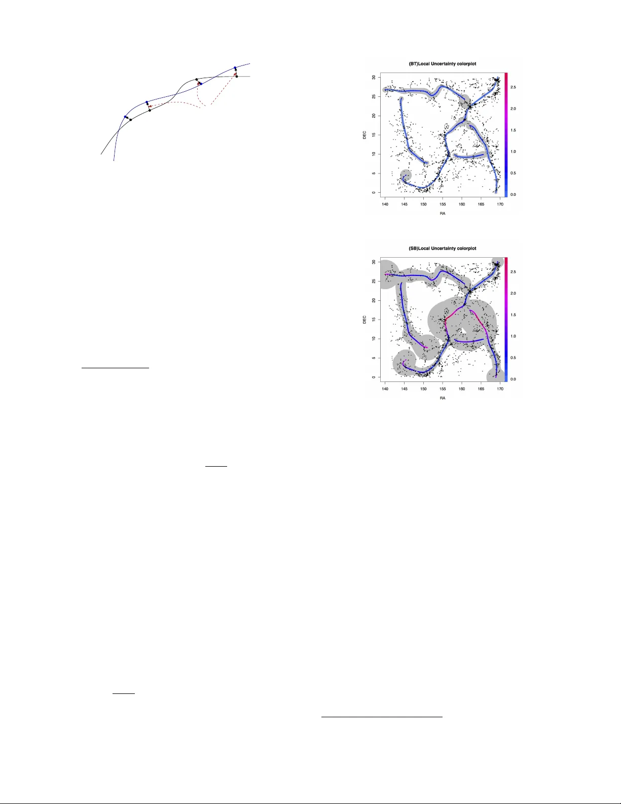
Uncer tainty Measures and Limiting Distrib utions f or Filament Estimation Y en-Chi Chen Carnegie Mellon Univ ersity 5000 F orbes A v e. Pittsburgh, P A 15213, USA yenchic@andre w .cmu.edu Christopher R. Genov ese Carnegie Mellon University 5000 Forbes A ve . Pittsburgh, P A 15213, USA genov ese@stat.cmu.edu Larr y W asserman Carnegie Mellon University 5000 Forbes A ve . Pittsburgh, P A 15213, USA larr y@stat.cmu.edu ABSTRA CT A filamen t is a high densit y , connected regi on in a p oin t cloud. There are sev eral metho ds for estimating filamen ts but these methods do not pro vide an y measure of uncer- tain ty . W e giv e a definition for the uncertain t y of estimated filamen ts and w e study statistical properties of the estimated filamen ts. W e sho w ho w to estimate the uncertain ty mea- sures and we construct confid ence sets based o n a b ootstrap- ping technique. W e apply our metho ds to astronomy data and earthquak e data. Categories and Subject Descriptors G.3 [ PROBABILITY AND ST A TISTICS ]: Multiv ari- ate statistics, Nonparametric statistics General T erms Theory K eywords filamen ts, ridges, density estimation, manifold learning 1. INTR ODUCTION A filamen t is a one-dimensional, smooth, connected struc- ture em b edded in a m ulti-dimensional space. Filamen ts arise in many applications. F or example, matter in the univ erse tends to concentrate near filaments that comprise what is kno wn as the cosmic-web [Bond et al. 1996], and the structure of that w eb can serv e as a tracer for estimat- ing fundamental cosmological constan ts. Other examples include neurofilamen ts and bloo d-v essel net works in neu- roscience [Lalonde and Strazielle 2003], fault lines in seis- mology [USGS 2003], and landmark paths in computer vi- sion [Hile et al. 2009]. Consider p oint-cloud data X 1 , X 2 , . . . , X n in R d , dra wn in- dependently from a densit y p with compact supp ort. W e define the filamen ts of the data distribution as the ridges of the probability densit y function p . (See Section 2.1 for Figure 1: Examples of p oint cloud data with ridges (filamen ts). details.) There are several alternative wa ys to formally de- fine filaments [Eberly 1996], but the definition we use has sev eral useful statistical prop erties [Genov ese et al. 2012d]. Figure 1 sho ws tw o simple examples of p oin t cloud data sets and the filaments estimated by our metho d. The problem of estimating filamen ts has been studied in sev eral fields and a v ariet y of metho ds ha v e b een dev el- oped, including parametric [Stoica et al. 2007, Stoica et al. 2008]; nonparametric [ Genov ese et al. 2012b, Geno ves e et al. 2012a, Geno vese et al. 2012c]; gradien t based [Geno vese et al. 2012d, Sousbie 2011, No vik ov et al. 2006]; and top o- logical [Dey 2006, Lee 1999, Cheng et al. 2005, Aanjaney a et al. 2012, Lecci et al. 2013]. While all these metho ds prov ide filamen t estimates, none pro vide an assessmen t of the estimate’s uncertain t y . That filamen t estimates are random sets is a significan t c hallenge in constructing v alid uncertaint y measures [Molchano v 2005]. In this pap er, we introduce a local uncertaint y measure for filamen t estimates. W e c haracterize the asymptotic distri- bution of estimated filamen ts and use it to derive consisten t estimates of the local uncertain ty measure and to construct v alid confidence sets for the filament based on b ootstrap re- sampling. Our main results are as follows: • W e show that if the data distribution is smooth, so are the estimated filamen ts (Theorem 1). • W e find the asymptotic distribution for es timated local uncertain ty and its con v ergence rate (Theorem 4, 5). • W e construct v alid and consistent , bo otstrap confi- dence sets for the local uncertain t y , and th us point wise confidence sets for the filament (Theorem 6). W e apply our methods to p oin t cloud data from ex amples in Astronom y and Seismology and demonstrate that they yield useful confidence sets. 2. B A CKGROUND 2.1 Density Ridges Let X 1 , · · · X n be random sample from a distribution with compact supp ort in R d that has densit y p . Let g ( x ) = ∇ p ( x ) and H ( x ) denote the gradien t and Hessian, respectively , of p ( x ). W e b egin by defining the ridges of p , as defined in [Geno v ese et al. 2012d, Ozertem and Erdogm us 2011, Eberly 1996]. While there are man y p ossible definitions of ridges, this definition giv es stabilit y in the underlying den- sit y , estimability at a go od rate of con v ergence, and fast reconstruction algorithms, as describ ed in [Geno v ese et al. 2012d]. In the rest of this paper, the filaments to b e esti- mated are just the one-dimensional ridges of p . A mo de of the density p – where the gradien t g is zero and all the eigen v alues of H are negative – can b e viewed as a zero-dimensional ridge. Ridges of dimension 0 < s < d generalize this to the zeros of a pr oje cte d gr adient where the d − s smallest eigenv alues of H are negativ e. In particular for s = 1, R ≡ Ridge( p ) = { x : G ( x ) = 0 , λ 2 ( x ) < 0 } , (1) where G ( x ) = V ( x ) V ( x ) T g ( x ) (2) is the pro jected gradien t. Here, the matrix V is defined as V ( x ) = [ v 2 ( x ) , · · · v d ( x )] for eigenv ectors v 1 ( x ) , v 2 ( x ) , ..., v d ( x ) of H ( x ) corresp onding to eigenv alues λ 1 ( x ) ≥ λ 2 ( x ) ≥ · · · ≥ λ d ( x ) Because one-dimensional ridges are the primary con- cern of this paper, we will refer to R in (1) as the “ridges” of p . In tuitively , at p oin ts on the ridge, the gradient is the same as the largest eigenv ector and the densit y curves do wn ward sharply in directions orthogonal to that. When p is smooth and the eigengap β ( x ) = λ 1 ( x ) − λ 2 ( x ) is positive, the ridges ha ve the all essential prop erties of filaments. That is, R decomposes in to a set of smooth curv e-lik e structures with high density and connectivity . R can also b e characterized through Morse theory [Guest 2001] as the collection of ( d − 1)-critical-points along with the local maxima, also kno wn as the set of 1-ascending manifolds with their lo cal-maxima limit p oin ts [Sousbie 2011]. 2.2 Ridge Estimation W e estimate the ridge in three steps: density estimation, thresholding, and ascent. First, we estimate p from from the data X 1 , . . . , X n . Here, we use the well-kno wn kernel densit y estimator (KDE) defined by b p n ( x ) = 1 nh d n X i =1 K  || x − X i || h  , (3) where the kernel K is a smo oth, symmetric density function suc h as a Gaussian and h ≡ h n > 0 is the bandwidth whic h con trols the smo othness of the estimator. Because ridge estimation can tolerate a fair degree of ov ersmo othing (as sho wn in [Genov ese et al. 2012d]), we select h by a simple rule that tends to o versmooth somewhat, the multiv ariate Silv erman’s rule [Silverman 1986]. Under w eak conditions, this estimator is consisten t; sp ecifically , || b p n − p || ∞ P → 0 as n → ∞ . (W e say that X n con verges in probabilit y to b , written X n P → b if, for ev ery  > 0, P ( | X n − b | >  ) → 0 as n → ∞ .) Second, w e threshold the estimated density to eliminate low- probabilit y regions and the spurious ridges produced in b p n b y random fluctuations. Here, we remov e p oin ts with esti- mated density less than τ || b p n || ∞ for a user-chosen threshold 0 < τ < 1. Finally , for a set of p oin ts ab ov e the densit y threshold, w e follo w the ascent lines of the pro jected gradien t to the ridge, whic h is the the subspace constrainted mean shift (SCMS) algorithm [Ozertem and Erdogmus 2011]. This pro cedure can be viewed as estimating the ridge b y applying the Ridge operator to b p n : b R n = Ridge( b p n ) . (4) Note that b R n is a random set. 2.3 Bootstrapping and Smooth Bootstrapping The b o otstrap [Efron 1979] is a statistical method for as- sessing the v ariabilit y of an estimator. Let X 1 , . . . , X n be a random sample from a distribution P and let θ ( P ) b e some functional of P to be estimated, such as the mean of the dis- tribution or (in our case) the ridge set of its densit y . Given some pro cedure b θ ( X 1 , . . . , X n ) for estimating θ ( P ) we es- timate the v ariabilit y of b θ by r esampling from the original data. Specifically , w e draw a bo otstr ap sample X ∗ 1 , . . . , X ∗ n inde- pendently and with replacement from the set of observed data p oin ts { X 1 , . . . , X n } and compute the estimate b θ ∗ = b θ ( X ∗ 1 , . . . , X ∗ n ) using the b o otstrap sample as if it w ere the data set. This process is rep eated B times, yielding B b ootstrap sam- ples and corresponding estimates b θ ∗ 1 , . . . , b θ ∗ B . The v ariabilit y in these estimates is then used to assess the v ariability in the original estimate b θ ≡ b θ ( X 1 , . . . , X n ). F or instance, if θ is a scalar, the v ariance of b θ is estimated by 1 B B X b =1 ( b θ ∗ b − θ ) 2 where θ = 1 B P B b =1 b θ ∗ b . Under suitable conditions, it can b e sho wn that this b ootstrap v ariance estimates – and confi- dence sets pro duced from it – are consistent. The smo oth b o otstr ap is a v arian t of the b ootstrap that can be useful in function estimation problems where the same procedure is used except the bo otstrap sample is dra wn from the estimated densit y b p instead of the original data. W e use both v arian ts below. 3. METHODS W e measure the lo c al unc ertainty in a filament (ridge) esti- mator b R n b y the exp ected distance b et wee n a sp ecified p oin t in the original filament R and the estimated filamen t: ρ 2 n ( x ) = ( E p d 2 ( x, b R n ) if x ∈ R 0 otherwise , (5) where d ( x, A ) is the distance function: d ( x, A ) = inf y ∈ A | x − y | . (6) The local uncertain t y measure can be understo od as the expected disp ersion for a giv en p oin t in the original filamen t to the estimated filament based on sample with size n . The theoretical analysis of ρ 2 n ( x ) is given in theorem 5. 3.1 Estimating Local Uncertainty Because ρ 2 n ( x ) is defined in terms unkno wn distribution p and the unknown filamen t set R , it must be estimated. W e use b ootstrap resampling to do this, defining an estimate of lo cal uncertaint y on the estimate d filaments . F or each of B bo otstrap samples, X ∗ ( b ) 1 , · · · , X ∗ ( b ) n , we compute the k ernel density estimator b p ∗ ( b ) n , the ridge estimate b R ∗ ( b ) n = Ridge( b p ∗ ( b ) n ), and the divergence ρ 2 ( b ) ( x ) = d 2 ( x, b R ∗ ( b ) n ) for all x ∈ b R n . W e estimate ρ 2 n ( x ) by b ρ 2 n ( x ) = 1 B B X b =1 ρ 2 ( b ) ( x ) ≡ E ( d 2 ( x, b R ∗ n ) | X 1 , · · · , X n ) , (7) for each x ∈ b R n , where the expectation is from the (known) bo otstrap distribution. Algorithm 1 provides pseudo-code for this pro cedure, and Theorem 6 sho ws that the estimate is consisten t under smo oth b ootstrapping. Algorithm 1 Lo cal Uncertaint y Estimator Input: Data { X 1 , . . . , X n } . 1. Estimate the filamen t from { X 1 , . . . , X n } ; denote the estimate by b R n . 2. Generate B b ootstrap samples: X ∗ ( b ) 1 , . . . , X ∗ ( b ) n for b = 1 , . . . , B . 3. F or each b ootstrap sample, estimate the filamen t, y ield- ing b R ∗ ( b ) n for b = 1 , . . . , B . 4. F or each x ∈ b R n , calculate ρ 2 ( b ) ( x ) = d 2 ( x, b R ∗ ( b ) n ), b = 1 , . . . , B . 5. Define b ρ 2 n ( x ) = mean { r 2 1 ( x ) , . . . , r 2 B ( x ) } . Output: b ρ 2 n ( x ). 3.2 Pointwise Confidence Sets Confidence sets provide another useful assessment of uncer- tain ty . A 1 − α confidence set is a random set comp uted from the data that conta ins an unknown quan tit y with at least probabilit y 1 − α . W e can construct a point wise confidence set for filaments from the distance function (6). F or each point x ∈ b R n , let r 1 − α ( x ) b e the (1 − α ) quantile v alue of d ( x, b R ∗ ) from the b ootstrap. Then, define C 1 − α ( X 1 , · · · , X n ) = [ x ∈ b R B ( x, r 1 − α ( x )) . (8) This confidence set capt ure the lo cal uncertaint y: for a point x ∈ b R n with lo w (high) lo cal uncertain ty , the asso ciated ra- dius r 1 − α ( x ) is small (large). But note that the confidence set attains 1 − α cov erage around each point; the co v erage of the en tire filament set is lo w er. That is, we can hav e high probabilit y to co v er each p oin t but the probabilit y to sim ul- taneously co v er all points (the whole filamen t set) migh t be lo wer. Algorithm 2 Poin twise Confidence Set Input: Data { X 1 , . . . , X n } ; significance level α . 1. Estimate the filament from { X 1 , . . . , X n } ; denote this b y b R n . 2. Generates bo otstrap samples { X ∗ ( b ) 1 , . . . , X ∗ ( b ) n } for b = 1 , . . . , B . 3. F or eac h bo otstrap sample, estimate the filament, call this b R ∗ ( b ) n . 4. F or each x ∈ b R n , calculate ρ 2 ( b ) ( x ) = d 2 ( x, b R ∗ ( b ) n ), b = 1 , . . . , B . 5. Let r 1 − α ( x ) = Q 1 − α ( ρ (1) ( x ) , . . . , ρ ( B ) ( x )). Output: S x ∈ b R n B ( x, r 1 − α ( x )) where B ( x, r ) is th e closed ball with center x and radius r . 4. THEORETICAL ANAL YSIS F or the filament set R , we assume that it can b e dec omp osed in to a finite partition { R 1 , · · · , R k } suc h that eac h R i is a one dimensional manifold. Suc h a partition can be constructed by the equation of trav ersal in page 56 of [Eb erly 1996]. F or each R i , we can parametrize it by a function φ i ( s ) : [0 , 1] → R i from the equation of tra versal men tioned with suitable scaling. F or simplicity , in the following pro ofs we assume that the filamen t set R is a single R i so that w e can construct the parametrization φ easily . All theorems and lemmas w e pro v e can b e applied to the whole filamen t set R = S i R i b y re- peating the process for eac h individual R i . 4.1 Smoothness of Density Ridges T o study the properties of the uncertain t y estimator, we first need to establish some results ab out the smo othness of the filamen t. The following theorem provides conditions for smoothness of the filamen ts. Let C k denote the collection of k times contin uously differen tiable functions. Theorem 1 (Smoothness of Filaments). L et φ ( s ) : [0 , 1] → R b e a p ar ameterization of filament set R , and for s 0 ∈ [0 , 1] , let U ⊂ R b e an op en set c ontaining φ ( s 0 ) . If p is C k and the eigengap β ( x ) > 0 for x ∈ U , then φ ( s ) is C k − 2 for s ∈ φ − 1 ( U ) . Theorem 1 sa ys that fi laments from a smo oth density will be smooth. Moreo ver, estimated filaments from the KDE will be smo oth if the k ernel function is smooth. In particular, if w e use Gaussian kernel, whic h is C ∞ , then the corresp ond- ing filamen ts will b e C ∞ as well. 4.2 Frenet Frame In the argumen ts that follow, it is useful to hav e a well- defined “mo ving” coordinate system along a smo oth curve. R e 1 ( s 1 ) e 2 ( s 1 ) e 2 ( s 2 ) e 1 ( s 2 ) e 1 ( s 3 ) e 2 ( s 3 ) Figure 2: An example for F renet frame in t w o di- mension. Let γ : R 7→ R d be an arc-length parametrization for a C k +1 curv e with k ≥ d . The F r enet frame [Kuhnel 2002] along γ is a smo oth family of orthogonal bases at γ ( s ) e 1 ( s ) , e 2 ( s ) , · · · e d ( s ) suc h that e 1 ( s ) = γ 0 ( s ) determines the direction of the curv e. The other basis elements e 2 ( s ) , · · · , e d ( s ) are called the cur- v ature vectors and can b e determined by a Gram-Schmidt construction. Assume the density is C d +3 . W e can construct a F renet frame for eac h p oint on the filamen ts. Let e 1 ( s ) , · · · , e d ( s ) be the F renet frame of φ ( s ) such that e 1 ( s ) = φ 0 ( s ) | φ 0 ( s ) | e j ( s ) = ˜ e j ( s ) | ˜ e j ( s ) | ˜ e j ( s ) = φ ( j ) ( s ) − j − 1 X i =1 < φ ( j ) ( s ) , e i ( s ) > e i ( s ) , j = 2 , · · · , d, where φ ( j ) ( s ) is the j th deriv ativ e of the φ ( s ) and < a, b > is the inner pro duct of vector a, b . An imp ortan t fact is that the basis element e j ( s ) is C d +3 − j , j = 1 , 2 · · · d . F renet frames are widely used in dynamical systems b ecause they pro vide a unique and con tin uous frame to describ e tra jecto- ries. 4.3 Normal space and distance measure The r e ach of R , denoted by κ ( R ), is the smallest real n um- ber r suc h that each x ∈ { y : d ( y , R ) ≤ r } has a unique pro jection onto R [F ederer 1959]. W e define the normal space L ( s ) of φ ( s ) by L ( s ) = n d X i =2 α i e i ( s ) ∈ R d : α 2 2 + · · · + α 2 d ≤ κ ( R ) 2 o . (9) Note that since we ha ve second deriv ativ e of φ ( s ) exists and finite, the reach will be b ounded from b elo w. Finally , define the Hausdorff distance b etw een tw o subsets of R d b y d H ( A, B ) = inf {  : A ⊂ B ⊕  and B ⊂ A ⊕  } , (10) where A ⊕  = S x ∈ A B ( x,  ) and B ( x,  ) = { y : k x − y k ≤  } . 4.4 Local uncertainty R L ( s 1 ) L ( s 2 ) φ ( s 1 ) φ ( s 2 ) e 2 ( s 1 ) e 3 ( s 1 ) e 2 ( s 2 ) e 3 ( s 2 ) Figure 3: An example for the normal space L ( s ) along a ridge in three dimensional. Let the estimated filamen t b e the ridge of KDE. W e assume the followi ng: (K1) The kernel K is C d +3 . (K2) The k ernel K satisfies condition K 1 in page 5 of [Gine and Guillou 2002]. (P1) The true density p is in C d +3 . (P2) The ridges of p ha ve positive reac h. (P3) The ridges of p are closed. F or example, Figure 1-(b). (K1) and (K2) are v ery m ild assumptions on the kernel func- tion. F or instance, Gaussain k ernels satisfy b oth. (P1-P3) are assumptions on the true densit y . (P1) is a smo othness condition. (P2) is a smo othness assumption on the ridge. (P3) is included to av oid b oundary bias when estimating the filamen t near endp oints . No w we introduce some norms and semi-norms c haracteriz- ing the smo othness of the density p . A v ector α = ( α 1 , . . . , α d ) of non-negativ e in tegers is called a m ulti-index with | α | = α 1 + α 2 + · · · + α d and corresponding deriv ative operator D α = ∂ α 1 ∂ x α 1 1 · · · ∂ α d ∂ x α d d , where D α f is often written as f ( α ) . F or j = 0 , . . . , 4, define k p k ( j ) ∞ = max α : | α | = j sup x ∈ R d | p ( α ) ( x ) | . (11) When j = 0, we ha ve the infinity norm of p ; for j > 0, these are semi-norms. W e also define k p k ∗ ∞ ,k = max j =0 , ··· ,k k p k ( j ) ∞ . (12) It is easy to verify that this is a norm. Next we recall a theorem in [Geno v ese et al. 2012d] whic h establish the link of Hausdorff distance b et ween R, b R n with the metric b et ween densit y . Theorem 2 (Theorem 6 in [Genovese et al. 2012d]). Under condi tions in [Genovese et al. 2012d], as || p − b p n || ∗ ∞ , 3 is sufficiently smal l , we have d H ( R, b R n ) = O P ( || p − b p n || ∗ ∞ , 2 ) . R d R n L ( s 1 ) L ( s 2 ) φ ( s 1 ) φ ( s 2 ) c φ n ( s 1 ) c φ n ( s 2 ) e 2 ( s 1 ) e 3 ( s 1 ) e 2 ( s 2 ) e 3 ( s 2 ) Figure 4: An example for b φ n ( s ) . This theorem tells us that w e hav e con vergence in Hausdorff distance for estimated filamen ts. Lemma 3 (Local p arametriza tion). F or the estimate d filament b R n , define b φ n ( s ) = L ( s ) ∩ b R n and ∆ n = d H ( b R n , R ) . Assume (K1), (K2), (P1), (P2). If || p − b p n || ∗ ∞ , 4 P → 0 , then, when ∆ n is sufficiently smal l, 1. b φ n ( s ) is a singleton for al l s exc ept in a set S n c on- taining the b oundaries with length ( S n ) ≤ O (∆ n ) . 2. d ( x, b R n ) −| φ ( s ) − b φ n ( s ) | | φ ( s ) − b φ n ( s ) | = o P (1) for x not at the bound ary of filaments. 3. If in addition (P3) holds, then S n = ∅ . Notice that a sufficient condition for Lemma 3 is nh d +8 log n → ∞ b y Lemma 8. Claim 1 follows b ecause the Hausdorff distance is less than min { κ ( R ) 2 , κ ( b R n ) 2 } . This will be true since b y Theorem 2, the Hausdorff distance is contolled by || p − b p n || ∗ ∞ , 2 , and we hav e a stronger con v ergence assumption. The only exception is points near the b oundaries of R since b R n can b e shorter than R in this case. But this can only occur in the set with length less than Hausdorff distance. Claim 2 follows from the fact that the normal space for φ ( s ) and b φ will b e asymptotically the same. If w e assume (P3), then R has no boundary , so that S n is an empty set. Note that Claim 2 gives us the v alidit y of approxima tion for d ( x, b R n ) via | φ ( s ) − b φ n ( s ) | . So the limiting bahavior of local uncertaint y d ( x, b R n ) will b e the same as | φ ( s ) − b φ n ( s ) | . In the follo wing, w e will study the limiting distributions for | φ ( s ) − b φ n ( s ) | . W e define the subsp ac e derivative by ∇ L = L T ∇ , which in turn gives the subsp ac e gr adient g ( x ; L ) = ∇ L p ( x ) and the subsp ac e Hessian H ( x ; L ) = ∇ L ∇ L p ( x ) . Then we hav e the follo wing theorem on lo cal uncertain ty , where X n d → Y denotes conv ergence in distribution. Theorem 4 (Local uncer t ainty theorem). Assume (K1),(K2),(P1),(P2). If nh d +8 log n → ∞ , nh d +10 → 0 , then √ nh d +2 ([ φ ( s ) − b φ n ( s )] − L ( s ) µ ( s ) h 2 ) d → L ( s ) A ( s ) wher e A ( s ) d = N (0 , Σ( s )) ∈ R d − 1 µ ( s ) = c ( K ) H ( φ ( s ); L ( s )) − 1 ∇ L ( s ) ( ∇ • ∇ ) p ( φ ( s )) Σ( s ) = H ( φ ( s ); L ( s )) − 1 ∇ L ( s ) K ( ∇ L ( s ) K ) T H ( φ ( s ); L ( s )) − 1 p ( φ ( s )) for al l φ ( s ) ∈ R \ S n with length ( S n ) ≤ O ( d H ( R, b R n )) . Theorem 4 states the asymptotic b eha vior of φ ( s ) − b φ n ( s ) whic h is asymptotically equiv alen t to lo cal uncertaint y . L ( s ) µ ( s ) h 2 is the bias component and L ( s ) A ( s ) is the sto c hastic v ari- ation comp onen t in whic h the parameter Σ( s ) con trols the amoun t of v aritaion. The con ten ts in parameters µ ( s ) and Σ( s ) link the geometry of the local densit y function with the local uncertain ty . Remarks: • Note that nh d +8 log n → ∞ is a sufficient condition for up to the fourth deriv ativ e unifo rm con v ergence. The uni- form conv egence in these deriv ativ e along with (P2) and theorem 1 ensures the reach of b R n will con v erge to the condition num ber of R . By theorem 4 and claim 2 in lemma 3, we know the asymp- totic distribution of local uncertaint y d ( x, b R n ). So we hav e the followi ng theorem on lo cal uncertaint y measure. Theorem 5. Define the lo c al unc ertatiny me asur e by ρ 2 n ( φ ( s )) = E ( d ( φ ( s ) , b R n ) 2 ) , wher e φ ( s ) r anges over al l p oints in R . Assume that (K1), (K2), (P1), and (P2) hold. If nh d +8 log n → ∞ , nh d +10 → 0 then ρ 2 n ( φ ( s )) = µ ( s ) T µ ( s ) h 4 + 1 nh d +2 T race(Σ( s ) 2 )+ o ( h 4 ) + o ( 1 nh d +2 ) , for al l φ ( s ) ∈ R \ S n with length ( S n ) ≤ O ( d H ( R, b R n )) . This theorem is just an application of theorem 4. How ever, it gives the conv ergence rate of lo cal uncertaint y measures. If we assume (P3), then Theorem 4, 5 can b e applied to all points on the filaments. 4.5 Bootstrapping Result F or the bo otstrapping result, we assume (P3) for conv e- nience. Note that if we do not assume (P3), the result still holds for p oin ts not close to terminals. Let q m be a sequence of densities satisfying (P1). W e w an t to study the local un- certain ty of the asso ciated filaments. So we wo rk on the random sample generated from q m and use the random sam- ple to build estimated filamen ts for filaments of q m . Define ψ m ( s ) , L ∗ m ( s ) as the a parametrization for the filaments and R ( p ) R ( q m ) φ ( s 1 ) φ ( s 2 ) φ ψ m ψ m ( ξ m ( s 1 )) ψ m ( ξ m ( s 2 )) ξ m Figure 5: An example for ξ m ( s ) along with φ, ψ m . associated normal space of q m . Then we ha v e the follo wing con vergence theorem for a sequence of densities con verging to p . Theorem 6. Assume that (P1–3) hold. Let q m b e a se- quenc e of pr ob ability densities that satisfy (P1), (P2), and k p − q m k ∗ ∞ , 3 → 0 as m → ∞ . If d H ( R ( q m ) , R ( p )) is sufficiently smal l, we c an find a bije c- tion ξ m : [0 , 1] 7→ [0 , 1] such that 1. | ψ m ( ξ m ( s )) − φ ( s ) | → 0 . 2.    <φ 0 ( s ) ,ψ 0 m ( ξ m ( s )) > | ψ 0 m ( ξ m ( s )) || φ 0 ( s ) |    → 1 . 3. sup s ∈ [0 , 1] | µ ( s ; q m ) − µ ( s ; p ) | → 0 . 4. sup s ∈ [0 , 1] | Σ( s ; q m ) − Σ( s ; p ) | → 0 . In p articular, if we use b p n = q n with nh d +8 log n → ∞ , nh d +10 → 0 , then the ab ove r esult holds with high pr ob ability. Note that the lo cal uncertain ty measure has unkno wn sup- port and unknown parameters giv en in theorem 5. Claim 1 shows the conv ergence in support while claim 3,4 prov e the consistency of the parameters control ling uncertain ties. This theorem states that if we hav e a sequence of densities con verging to a limiting density , then the local uncertaint y will conv erge in a sense. Remarks: • Notice that ψ m ( ξ m ( s )) need not b e the same as L ( s ) ∩ R ( q m ). The latter one liv es in the normal space of φ ( s ) but the former need only be a contin uously bijectiv e mapping. The pro jection that maps s to the p oint L ( s ) ∩ R ( q m ) is one choice of ξ m . • The last result holds immediately from Lemma 8 as w e pic k nh d +8 log n → ∞ , nh d +10 → 0. The bandwidth in this case will ensure uniform con vergence in probability up to the forth deriv ative which is sufficien t to the condition. (a) Bootstrapping (b) Smooth b o otstrapping Figure 6: Lo cal uncertaint y measures and p oint- wise confidence sets for SDSS data. (a): Bo otstrap- ping result. (b): Smo oth b ootstrapping result. W e displa y lo cal uncertaint y measures based on color (red: high uncertaint y) and 90% p oin t wise confi- dence sets. 5. EXAMPLES W e apply our methods to t wo datasets, one from astronom y and one from seismology . In both cases, w e use an isotropic Gaussian kernel for the KDE and threshold using τ = 0 . 1. W e use a 50 × 50 uniform grid o ver each sample as initial points in the ascent step for running SCMS. W e compare t he result from b ootstrapping and smo oth b ootstrapping based on 100 b ootstrap samples to estimate uncertaint y . Astr onomy Data. The data come from Slo an Digit Sky Sur- vey(SDSS) Data R ele ase(DR) 9 . 1 In this dataset, each point is a galaxy and is characterized by three features ( z, r a, de c ). z is the redshift v alue, a measurement of the distance form that galaxy to us. r a is right ascesion, the latitude of the sky . de c is declination, the longitude of the sky . W e restrict ourselves to z=0.045 ∼ 0.050 which is a slice of data on the z co ordinate that consists of 2 , 532 galaxies. W e selected v alues in (r a, de c)=(0 ∼ 30, 140 ∼ 170) . The 1 The SDSS dataset http://w ww.sdss3.org/dr9/ bandwidth h is 2.41. Figure 6 displays the local uncertain t y measures with p oint- wise confidence sets. The red color indicates higher lo- cal uncertaint y while the blue color stands for low er uncer- tian ty . Bo otstrapping shows a v ery small lo cal uncertain ty and very narrow point wise confidence sets. Smo oth b oot- stapping yields a loose confidence sets but it shows a clear pattern of local uncertaint y whic h can b e explained by our theorems. F rom Figure 6, w e identify four cases associated with high local uncertaint y: high curv ature of the filament, flat den- sit y near filamen ts, terminals (boundaries) of filaments, and in tersecting of filamen ts. F or the p oints near curved fila- men ts, we can see uncertain ty increases in every case. This can b e explained by theorem 4. The curv ature is related to the third deriv ativ e of densit y from the definition of ridges. F rom theorem 4, w e kno w the bias in filament estimation is proportional to the third deriv ativ e. So the estimation for highly curv ed filamen ts tends to hav e a systematic bias in filamen t estimation and our uncertaint y measure captures this bias successfully . F or the case of a flat densit y , by theorem 4, w e know b oth the bias and v ariance of local uncertain ty is prop ortional to the in verse of the Hessian. A flat densit y has a very small Hes- sian matrix and thus the inv erse will b e huge; this raises the uncertain ty . Though our theorem can not b e applied to ter- minals of filamen ts, w e can still explain the high u ncertiant y . P oints near terminals suffer from b oundary bias in densit y estimation. This leads to an increase in the uncertain ty . F or regions near connections, the eigengap β ( x ) = λ 1 ( x ) − λ 2 ( x ) will approach 0 which causes instabilit y of the ridge since our definition of ridge requires β ( x ) > 0. All cases with high local uncertain ty can be explained b y our theoretical result. So the data analysis is consistent with our theory . Earthquake Data . W e also apply our tec hnique to data from the U.S. Geological Surv ey 2 that lo cates 1 , 169 earthquakes hat occur in region b et ween longitude (100 E ∼ 160 E ), lat- itude (0 N ∼ 60 N ) and in dates b etw een 01/01/2013 to 09/30/2013. W e are particularly interested in detecting plate boundaries, whic h see a high incidence of earthquakes. W e pre-process the data to remo v e a cluster of earthquakes that are irrelev an t to the plate boundary . F or this data, we only consider those filamen ts with density larger than τ = 0 . 02 of the maximum of the densit y . Because the noise level is sm all, w e adjust the KDE bandwidt h to 0 . 7 times the Silverman rule ( h = 2 . 83). Figure 7 displays the estimated filaments and 90% point wise confidence sets. The Figure shows the true plate boundaries from Nuv el data set 3 as bro wn p oin ts. As can b e seen in the Figure, smo oth bo otstrapping has b etter cov erage ov er the plate b oundary . W e notice the bad cov erage in the b ottom part; this is reasonable since the b oundary bias and lack of data cause trouble in estimation and uncertaint y mea- sures. W e also identify some parts of filaments with high local uncertain t y . The filaments with high uncertaint y can 2 The USGS dataset h ttp://earthquak e.usgs.gov/earthqua kes/searc h/ 3 Nuv el data set http://www.earth b yte.org/ (a) Bootstrapping (b) Smooth b o otstrapping Figure 7: Earthquak e data. This is a collection of earthquak e data in longitude (100 ∼ 160) E , lattitude (0 ∼ 60) N from 01/01/2013 to 09/30/2013. T otal sample size is 1169 . Blue curves are the estimated filamen ts; brown dots are the plate b oundaries. be explained by theorem 4. The data analysis again support our theoretical result. In both Figure 6, 7, we see a clear picture on the uncertain t y assessmen t for filament estimation. In data from t w o or three dimension, w e can visua lize uncertain ties in estimation of filamen ts with different colors or c onfidence regions. That is, w e can d isplay estimation and the uncertaint y in the same plot. 6. DISCUSSION AND FUTURE WORK In this paper, we define a lo cal uncertaint y measure for fila- men t estimation and study its theoretical prop erties. W e apply bo otstrap resampling to estimate lo cal uncertaint y measures and construct confidence sets, and we pro ve that both are consistent and data analysis also supp orts our re- sult. Our method pro vides one w ay to numerically quantify the uncertaint y for estimating filaments. W e also visualize uncertatin y measures with estimated filaments in the same plot; this can b e one easy wa y to show estimation and the uncertain ty sim ultaneously . Our approac h has no constraint s on the dimension of the data so it can b e extended to data from higher dimension (although the confidence sets will b e larger). Our defini- tion of lo cal uncertain ty and our estimation method can b e applied to other geometric estimation algorithms, which w e will inv estigate in the future. APPENDIX A. PR OOFS Proof of Theorem 1. F or the ridge set R , it is a collec- tion of solutions to G ( x ) = V ( x ) V ( x ) T ∇ p ( x ) as the eigengap β ( x ) > 0. But V ( x ) is a d × ( d − 1) o rthonormal basis. So the solution to G ( x ) = V ( x ) V ( x ) T ∇ p ( x ) = 0 is equal to the so- lution to F ( x ) = V ( x ) T ∇ p ( x ) = 0. No w F ( x ) : R d 7→ R d − 1 . Hence, implicit function theorem tells us that the differen- tiablilt y of a lo cal graph { ( z , g ( z )) : z ∈ R , g ( z ) ∈ R d − 1 } is the same as F ( x ) when β ( x ) > 0. Now since the lo cal graph is parametrized b y one v ariable, w e can reparametrize it b y a curve φ ( x ). And the differen tiability of the curv e is the same as F ( x ). F rom a slight modification from theorem 3 in [Genov ese et al. 2012d], the k th order deriv ativ e of F ( x ) dep ends on k + 2th order deriv ativ e of densit y if the eigengap β ( x ) > 0. Hence, if the densit y is C k and we consider an op en set U with β ( x ) > 0 ∀ x ∈ U , then w e ha v e F ( x ) is C k − 2 on U so the result follo ws.  T o prov e theorem 4, we need the follo wing lemmas: Lemma 7. L et b p n ( x ) b e KDE for p ( x ) . Assume our ker- nel satisfies (K1), (K2). If nh d +2 → ∞ , nh d +10 → 0 , h → 0 . Then ∇ b p n ( x ) admits an asymptotic normal distribution by √ nh d +2 ( ∇ b p n ( x ) − ∇ p ( x ) − B ( x ) h 2 ) d → N (0 , Σ 0 ( x )) (13) wher e B ( x ) = m 2 ( K ) 2 ∇ ( ∇ • ∇ ) p ( x ) (14) Σ 0 ( x ) = ∇ K ( ∇ K ) T p ( x ) (15) K is the kernel use d and m 2 ( K ) is a c onstant of kernel. Proof. F or KDE b p n , b p n ( x ) = 1 n n X i =1 1 h d K ( x − X i h ) . (16) Hence for ∇ b p n , ∇ b p n = 1 n n X i =1 1 h d ∇ K ( x − X i h ) = 1 n n X i =1 Φ( x ; X i ) . Notice that each Φ( x ; X i ) is indep endent and iden tically dis- tributed. W e will sho w that Φ( x ; X i ) satisfies conditions for Lyapounov’s condition so that we ha ve Cen tral Limit Theorem (CL T) re- sult for it. WLOG, we consider the third moment and fo cus on partial deriv ativ e o ver a direction, sa y j , w e wan t ( n E ( | Φ j ( x ; X i ) − E (Φ j ( x ; X i )) | 3 )) 1 3 ( nV ar (Φ j ( x ; X i ))) 1 2 → 0 (17) where Φ j ( x ; X i ) = 1 h d ∂ ∂ x j K ( x − X i h ) = 1 h d +1 ∂ K ∂ x j ( x − X i h ). This is equiv alen t to show n 2 E ( | Φ j ( x ; X i ) − E (Φ j ( x ; X i )) | 3 ) 2 n 3 V ar (Φ j ( x ; X i )) 3 → 0 (18) No w we put an upper bound on (18), then w e hav e n 2 E ( | Φ j ( x ; X i ) − E (Φ j ( x ; X i )) | 3 ) 2 n 3 V ar (Φ j ( x ; X i )) 3 ≤ n 2 E ( | Φ j ( x ; X i ) | 3 ) 2 n 3 V ar (Φ j ( x ; X i )) 3 . W e assume that R ( ∂ K ∂ x j ( u )) 2 du = C 2 < ∞ , R ( ∂ K ∂ x j ( u )) 3 du = C 3 < ∞ for all j = 1 , · · · , d . Therefore b y T a ylor expansion o ver densit y and take the first order, we ha v e n 2 E ( | Φ j ( x ; X i ) | 3 ) 2 n 3 V ar (Φ j ( x ; X i )) 3 = n 2 ( C 3 p ( x ) h 2 d +3 + o ( 1 h 2 d +3 )) 2 n 3 ( C 2 p ( x ) h d +2 + o ( 1 h d +2 )) 3 = O ( 1 nh d ) = o (1) As a result, Ly ap ouno v’s condition is satisfied and this holds for all j = 1 , · · · , d ; so w e hav e CL T for Φ( x ; X i ). By multiv ariate CL T we ha ve V ar (Φ( x ; X i )) − 1 2 [ ∇ b p n − E (Φ( x ; X i ))] d → N (0 , I d ) . where I d is the identit y matrix of dimension d . By theorem 4 in [Chac´ on et al. 2011], we ha v e E (Φ( x ; X i )) = ∇ p ( x ) + m 2 ( K ) 2 ∇ ( ∇ • ∇ ) p ( x ) h 2 + O ( h 4 ) = ∇ p ( x ) + B ( x ) h 2 + O ( h 4 ) V ar (Φ( x ; X i )) = 1 nh d +2 ∇ K ( ∇ K ) T p ( x ) + o ( 1 nh d +2 ) = Σ 0 ( x ) nh d + o ( 1 nh d ) Therefore, as nh d +2 → ∞ and h → 0, √ nh d +2 Σ 0 ( x ) − 1 2 ( ∇ b p n ( x ) − ∇ p ( x ) − B ( x ) h 2 − O ( h 4 )) d → N (0 , I d ) No w since nh d +10 → 0 so √ nh d +2 O ( h 4 ) tends to 0 and m ultiply Σ 0 ( x ) 1 2 in b oth side, w e get √ nh d +2 ( ∇ b p n ( x ) − ∇ p ( x ) − B ( x ) h 2 ) d → N (0 , Σ 0 ( x )) This completes the pro of.  Lemma 8. ([Gine and Guillou 2 002]; version of [Geno v ese et al. 2012d]) Assume (K1), (P1) and the kernel function satisfies c ondi- tions in [Gine and Guil lou 2002]. Then we have || b f n,h − f || ∞ ,k = O ( h 2 ) + O P ( log n nh d +2 k ) . (19) Lemma 9. F or a density p , let R b e its filaments. F or any p oints x on R , let the Hessian at x b e H ( x ) with eigen- ve ctors [ v 1 , · · · , v d ] and eigenvalues λ 1 > 0 > λ 2 ≥ · · · λ d . Consider any subsp ac e L sp anne d by a b asis [ e 2 , · · · e d ] with e 1 b e the normal ve ctor for L . Then a sufficient and ne c es- sary c ondition for x b e a lo c al mo de of p c onstr aine d in L is d X i =1 λ i ( v T i e j ) 2 < 0 , ∀ j = 2 , · · · , d. (20) A sufficient c ondition for (20) is ( v T 1 e 1 ) 2 > λ 1 λ 1 − λ 2 . (21) Proof. Let the Hessian of density p at x b e H ( x ) with eigen vectors [ v 1 , · · · , v d ] and asso ciated eigen v alues λ 1 ≥ λ 2 ≥ · · · λ d . Consider an y subspace L spanned b y a basis [ e 2 , · · · e d ] with e 1 be the normal vecto r for L F or any x on the ridge, we hav e λ 1 > 0 > λ 2 . x is the mode constrained in the subspace L if ∇ L ∇ L p ( x ) is negative definite. By sp ectral decomposition, we can write ∇ L ∇ L p ( x ) = L T H ( x ) L = L T U ( x )Ω( x ) U ( x ) L T , where U ( x ) = [ v 1 , · · · , v d ] and Ω( x ) is a diagonal matrix of eigen v alues. So this matrix will b e negativ e definite if and only if all its diagonoal elements are negativ e. That is, the sufficient and necessary condition is ( ∇ L ∇ L p ( x )) ii < 0 , i = 1 , · · · , d − 1 . (22) W e explicitly deriv e the form of (22) and consider the suffi- cien t and necessary condition: ( ∇ L ∇ L p ( x )) j j = ( L T U ( x )Ω( x ) U ( x ) L T ) j j = d X i =1 e T j v i λ i v T i e j = d X i =1 λ i ( v T i e j ) 2 < 0 , j = 2 , · · · d. So we pro v e the first condition. T o see the sufficien t condition, w e note that b y definition, λ 2 ( x ) ≥ · · · ≥ λ d ( x ). So for each j , d X i =2 λ i ( v T i e j ) 2 ≤ λ 2 d X i =2 ( v T i e j ) 2 . This implies that for each j , d X i =1 λ i ( v T i e j ) 2 ≤ ( λ 1 − λ 2 )( v T 1 e j ) 2 + λ 2 d X i =1 ( v T i e j ) 2 = ( λ 1 − λ 2 )( v T 1 e j ) 2 + λ 2 < 0 . Note that we use the fact P d i =1 ( v T i e j ) 2 = 1 since | e j | = 1 and v i ’s are basis. Since b oth e 1 , · · · , e d and v 1 , · · · , c d are basis, we ha v e ( v T 1 e j ) 2 ≤ 1 − ( v T 1 e 1 ) 2 for all j = 2 , · · · , d . Then we further hav e ( λ 1 − λ 2 )( v T 1 e j ) 2 + λ 2 ≤ ( λ 1 − λ 2 )(1 − ( v T 1 e 1 ) 2 ) + λ 2 = − ( λ 1 − λ 2 )( v T 1 e 1 ) 2 + λ 1 for each j = 2 , · · · d . Putting altogether, w e hav e ( ∇ L ∇ L p ( x )) j j = d X i =2 λ i ( v T i e j ) 2 ≤ ( λ 1 − λ 2 )( v T 1 e j ) 2 + λ 2 ≤ − ( λ 1 − λ 2 )( v T 1 e 1 ) 2 + λ 1 < 0 for all j = 2 , · · · , d So a sufficient condition is ( v T 1 e 1 ) 2 > λ 1 ( λ 1 − λ 2 ) .  Proof of Theorem 4. By definition of φ ( s ) , b φ ( s ) and the nature of ridge, φ ( s ) is the lo cal mo de of p ( x ) in the subspace spanned by L ( s ) near φ ( s ). By lemma 9, b φ ( s ) will also the local mo de of b p n ( x ) in the subspace spanned by L ( s ) near φ ( s ) once the tw o filamnets are closed enough and the local direction of filament s are also closed. This will be sho wn in 2. of theorem 6. Hence, we hav e ∇ L ( s ) p ( φ ( s )) = ∇ L ( s ) b p n ( b φ n ( s )) = 0 . No w applying T aylor expansion for ∇ L ( s ) b p n ( b φ n ( s )) near φ ( s ), we ha v e 0 = ∇ L ( s ) b p n ( b φ n ( s )) = ∇ L ( s ) b p n ( φ ( s )) + b H L ( s ) n ( φ ∗ ( s )) L ( s ) T ( b φ n ( s ) − φ ( s )) where b H n ( x ; L ( s )) is the pro jected Hessian of KDE while φ ∗ ( s ) = tφ ( s ) + (1 − t ) b φ ( s ), for some 0 ≤ t ≤ 1. Accordingly , L ( s ) T ( b φ n ( s ) − φ ( s )) = − b H n ( φ ∗ ( s ); L ( s )) − 1 ∇ L ( s ) b p n ( φ ( s )) . (23) By lemma 8 with k = 2 and w e pick a suitable h = h n , we ha ve b H n ( φ ∗ ( s )) p → H ( φ ∗ ( s )) whic h implies b H n ( φ ∗ ( s ); L ( s )) p → H ( φ ∗ ( s ); L ( s )) and φ ∗ ( s ) will conv erge to φ ( s ). Consequen tly , b H n ( φ ∗ ( s ); L ( s )) p → H ( φ ( s ); L ( s )) . This implies b H n ( φ ∗ ( s ); L ( s )) − 1 p → H ( φ ( s ); L ( s )) − 1 (24) since H ( x ) is non-singular. No w we consider ∇ L ( s ) b p n ( φ ( s )). Recall that we assume nh d +2 → ∞ , nh d +10 → 0 , h → 0; b y lemma 7 we ha ve √ nh d +2 ( ∇ b p n ( φ ( s )) − ∇ p ( φ ( s )) | {z } =0 (local mode) − B ( φ ( s )) h 2 ) d → N (0 , Σ 0 ( φ ( s ))) with B ( φ ( s )) = m 2 ( K ) 2 ∇ ( ∇ • ∇ ) p ( φ ( s )) Σ 0 ( s ) = ∇ K ( ∇ K ) T p ( φ ( s )) . Hence, for the subspace case: √ nh d +2 ( L ( s ) T ∇ b p n ( φ ( s )) − L ( s ) T B ( φ ( s )) h 2 ) d → N (0 , L ( s )Σ 0 ( φ ( s )) L ( s ) T ) (25) Recalled (23) : L ( s ) T ( b φ n ( s ) − φ ( s )) = − b H n ( φ ∗ ( s ); L ( s )) − 1 ∇ L ( s ) b p n ( φ ( s )) = b H n ( φ ∗ ( s ); L ( s )) − 1 L ( s ) T ∇ b p n ( φ ( s )) no w we plug in (25) and apply Slutsky’s theorem, we get √ nh d +2 [ L ( s ) T ( b φ n ( s ) − φ ( s )) − µ ( s ) h 2 ] d → N (0 , Σ( s )) (26) where µ ( s ) = H ( φ ( s ); L ( s )) − 1 L ( s ) T B ( φ ( s )) Σ( s ) = H ( φ ( s ); L ( s )) − 1 L ( s )Σ 0 ( φ ( s )) L ( s ) T H ( φ ( s ); L ( s )) − 1 . No w since b φ n ( s ) − φ ( s ) alw a ys lays in the subspace L ( s ), we ha ve L ( s ) L ( s ) T ( b φ n ( s ) − φ ( s )) = b φ n ( s ) − φ ( s ) . Consequen t, we can m ultiply L ( s ) in (26) to obtain √ nh d +2 [( b φ n ( s ) − φ ( s )) − L ( s ) µ ( s ) h 2 ] d → L ( s ) A ( s ) with A ( s ) d = N (0 , Σ( s )) ∈ R d − 1 is a Gaussian pro cess in R d − 1 .  Proof of Theorem 6. 1. By assumption, the ridges for p and q m ha ve p ositive conditioning num ber. W e can apply theorem 6. in Genov ese et. al. (2012) so that R ( p ) and R ( q m ) will b e asymptotically top ological homotop y . So we can alwa ys find a contin uous bijective mapping to map every point on R ( p ) to R ( q m ). W e define ξ m be such a map on eac h point of R ( p ). Since the Hausdorff distance co nv erge to 0, the associated mapping can be pick ed such that each pair φ ( s ) , ψ m ( ξ m ( s ) has distance less than Hausdorff distance. So the result follows. 2. Recall that filaments are solutions to { x : V ( x ) V ( x ) T ∇ p ( x ) = 0 , β ( x ) > 0 } . The direction of ridge ( φ ( s ) , ψ 0 m ( s )) depends on up to third deriv ativ e at p oin ts on the filaments. F rom 1., w e know that the lo cation of ψ m ( ξ m ( φ ( s ))) will conv erge to φ ( s ) and w e hav e the uniform con vergence up to the third deriv ativ e b y assumptions. Hence, b y uniformly con v ergence and b oth p, q m are C d +3 , we hav e conv ergence in the tangen t line at eac h point of filaments. So this implies the inner product to be 1. 3. F rom theorem 4, µ ( s ) = c ( K ) H ( φ ( s ); L ( s )) − 1 ∇ L ( s ) ( ∇ • ∇ ) p ( φ ( s )). By assumption, we hav e uniform con vergence up to third deriv ative and by 2. we hav e conv ergence in subspace. So µ ( s ) from q m will unifromly con verge to that from p . 4. Similar to 3.  B. REFERENCES [Aanjaney a et al. 2012] Mridul Aanjaney a, F rederic Chazal, Daniel Chen, Marc Glisse, Leonidas Guibas, and Dmitriy Morozov . 2012. Metric graph reconstruction from noisy data. International Journal of Computational Ge ometry and and Applic ations (2012). [Bond et al. 1996] J. R. Bond, L. Kofman, and D. P ogosyan. 1996. Ho w filamen ts of galaxies are wo ven in to the cosmic web. Natur e (1996). [Chac´ on et al. 2011] J.E. Chac´ on, T. Duong, and M.P W and. 2011. Asymptotics for general multiv ariate k ernel density deriv ative estimators. Statistic a Sinic a (2011). [Cheng et al. 2005] S.-W. Cheng, S. F unke, M. Golin, P . Kumar, S.-H. Poon, and E. Ramos. 2005. Curve reconstruction from noisy samples. In Computational Ge ometry 31 . [Dey 2006] T. Dey. 2006. Curve and Surfac e R e c onstruction: Algor ithms with Mathematic al Ana lysis. Cambridge Univ ersit y Press. [Eberly 1996] David Eberly. 1996. Ridges in Image and Data A nalysis . Springer. [Efron 1979] B. Efron. 1979. Bo otstrap Metho ds: Another Look at the Jac kknife. A nnals of Statistics 7, 1 (1979), 1–26. [F ederer 1959] H. F ederer. 1959. Curv ature measures. T r ans. A m. Math. So c 93 (1959). [Geno vese et al. 2012a] Christopher R. Genov ese, Marco P erone-Pacifico, Isabella V erdinelli, and Larry W asserman. 2012a. The geometry of nonparametric filamen t estimation. J. Amer. Statist. Asso c. (2012). [Geno vese et al. 2012b] Christopher R. Genov ese, Marco P erone-Pacifico, Isabella V erdinelli, and Larry W asserman. 2012b. Manifold estimation and singular decon volution under hausdorff loss. The Annals of Statistics (2012). [Geno vese et al. 2012c] Christopher R. Genov ese, Marco P erone-Pacifico, Isabella V erdinelli, and Larry W asserman. 2012c. Minimax manifold estimation. Journal of Machine L e arning R ese ar ch (2012). [Geno vese et al. 2012d] Christopher R. Genov ese, Marco P erone-Pacifico, Isabella V erdinelli, and Larry W asserman. 2012d. Nonparametric ridge estimation. arXiv:1212.5156v1 (2012). [Gine and Guillou 2002] E. Gine and A Guillou. 2002. Rates of strong uniform consistency for multiv ariate k ernel density estimators. In Annales de l’Institut Henri Poincar e (B) Pr ob ability and Statistics (2002). [Guest 2001] Martin A. Guest. 2001. Morse theory in the 1990’s. arXiv:math/0104155v1 (2001). [Hile et al. 2009] Harlan Hile, Radek Grzeszczuk, Alan Liu, Ramakrishna V edantham, Jana Ko ˇ sec k a, and Gaetano Borriello. 2009. Landmark-Based P edestrian Na vigation with Enhanced Spatial Reasoning. L e ctur e Notes in Computer Scienc e 5538 (2009). [Kuhnel 2002] W olfgang Kuhnel. 2002. Differ ential ge ometry: curves-surfac es-manifolds . V ol. 16. studen t mathematical library . [Lalonde and Strazielle 2003] R. Lalonde and C. Strazielle. 2003. Neurobehavioral c haracteristics of mice with modified in termediate filament genes. R ev Neur osci (2003). [Lecci et al. 2013] F abrizio Lecci, Alessandro Rinaldo, and Larry W asserman. 2013. Statistical Analysis of Metric Graph Reconstruction. arXiv:1305.1212 (2013). [Lee 1999] I.-K. Lee. 1999. Curve reconstruction from unorganized points.. In Computer Aide d Ge ometric Design 17 . [Molc hanov 2005] I. Molc hano v. 2005. The ory of random sets . Springer-V erlag London Ltd. [No viko v et al. 2006] D. Novik ov, S. Colom bi, and O. Dore. 2006. Skeleton as a prob e of the cosmic w eb: the t wo-dimensional case. Mon. Not. R. Astr on. So c. (2006). [Ozertem and Erdogmu s 2011] Um ut Ozertem and Deniz Erdogm us. 2011. Locally Defined Principal Curves and Surfaces. Journal of Machine L e arning R ese ar ch (2011). [Silv erman 1986] B. W Silv erman. 1986. Density Estimation for Statistics and Data Anal ysis . Chapman and Hall. [Sousbie 2011] T. Sousbie. 2011. The persistent cosmic web and its filamentary structure – I. Theory and implemen tation. Mon. Not. R. Astr on. So c. (2011). [Stoica et al. 2007] R. Stoica, V. Martinez, and E. Saar. 2007. A three-dimensional ob ject p oint process for detection of cosmic filament s. Appl. Statist. (2007). [Stoica et al. 2008] R. S. Stoica, V. J. Mart ` I  A ¨ A ´ snez, J. Mateu, and E. Saar. 2008. Detection of cosmic filamen ts using the Candy mo del. A. and A. (2008). [USGS 2003] USGS. 2003. Wher e ar e the F ault Lines in the Unite d States East of the R o cky Mountains?