Stochastic Convergence of Persistence Landscapes and Silhouettes

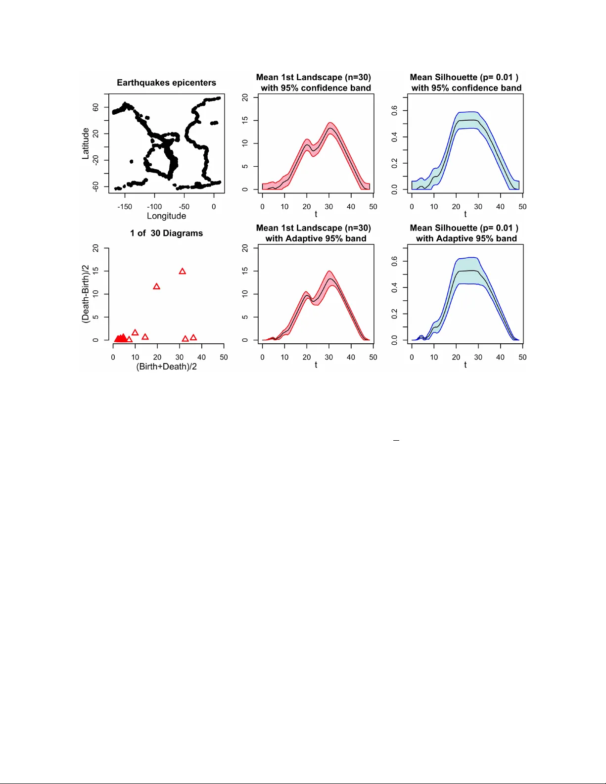
Stochastic Convergence of P ersistence Landscapes and Silhouettes Frédéric Chazal 1 , Brittany T erese F asy 2 , F abrizio Lecci 3 , Alessandro Rinaldo 3 , and Larry W asserman 3 1 INRIA Saclay 2 Computer Science Department, T ulane University 3 Department of Statistics , Carnegie Mellon University topstat@stat.cmu.edu November 27, 2013 Abstract P ersistent homology is a widely used tool in T opological Data Analysis that encodes multiscale topological information as a multi-set of points in the plane called a persistence diagram. It is difficult to apply statistical theory directly to a random sample of diagrams . Instead, we can sum- marize the persistent homology with the persistence landscape, introduced by Bubenik, which converts a diagram into a well-behaved real-valued function. W e investigate the statistical prop- erties of landscapes, such as weak convergence of the average landscapes and convergence of the bootstrap. In addition, we introduce an alternate functional summary of persistent homology , which we call the silhouette, and derive an analogous statistical theory . 1 1 Introduction Often, data can be represented as point clouds that carry specific topological and geometric struc- tures . Identifying, extracting, and exploiting these underlying geometric structures has become a problem of fundamental importance for data analysis and statistical learning. With the emergence of new geometric inference and algebraic topology tools, computational topology has recently seen an important development toward data analysis, giving birth to the field of T opological Data Anal- ysis , whose aim is to infer relevant, multiscale, qualitative, and quantitative topological structures directly from the data. P ersistent homology (Edelsbrunner et al. (2002); Zomorodian and Carlsson (2005)) is a fundamental tool for providing multi-scale homology descriptors of data. More precisely , it provides a framework and efficient algorithms to quantify the evolution of the topology of a family of nested topological spaces , { X ( t ) } t ∈ R , built on top of the data and indexed by a set of real numbers – that can be seen as scale parameters – such that X ( t ) ⊆ X ( s ) for all t ≤ s . At the homology level 1 , such a filtration induces a family { H ( X ( t )) } t ∈ R of homology groups and the inclusions X ( t ) , → X ( s ) induce a family of homomorphisms H ( X ( t )) → H ( X ( s )), t ≤ s , which is known as the persistence module associated to the filtration. When the rank of all the homomorphisms H ( X ( t )) → H ( X ( s )), t < s , are finite the module is said to be q-tame (Chazal et al. (2012)) and it can be summarized as a set of real intervals ( b i , d i ) representing homological features that appear in the filtration at t = b i and disappear at t = d i . Such a set of intervals can be represented as a multi-set of points in the real plane and is then called a persistence diagrams . Thanks to their stability properties (Cohen-Steiner et al. (2007); Chazal et al. (2012)), persistence diagrams provide relevant multi-scale topological information about the data. In a more statistical framework, when several data sets are randomly generated or are coming from repeated experiments , one often has to deal with not only one persistence diagrams but with a whole distribution of persistence diagrams . Unfortunately , since the space of persistence diagrams is a general metric space, analyzing and quantifying the statistical properties of such a distribution turns out to be particularly difficult. A few attempts have been made towards a statistical analysis of distributions of persistence dia- grams . F or example, the concentration and convergence properties of persistence diagrams obtained from point cloud randomly sampled on manifolds and from more general compact metric spaces are studied in Balakrishnan et al. (2013); Chazal et al. (2013b). Considering general distributions of persistence diagrams, Turner et al. (2012) have suggested using the F réchet average of the diagrams D 1 , . . . , D n . Unfortunately , the Fréchet a verage is unstable and not even unique . A solution that uses a probabilistic approach to define a unique Fréchet average can be found in Munch et al. (2013), but its computation remains practically prohibitive. In this paper , we also consider general distributions of persistence diagrams but we build on a com- pletely different approach, proposed in Bubenik (2012), consisting of encoding persistence diagrams as a collection of real-valued one-Lipschitz functions that are called persistence landscapes; see Sec- tion 2. The advantage of landscapes — and, more generally , of any function-valued summaries of persistent homology — is that we can analyze them using existing techniques and theories from nonparametric statistics . W e have in mind two scenarios where multiple persistence diagrams arise: 1 W e consider here homology with coefficient in a given field, so the homology groups are vector spaces. 2 Scenario 1: W e have a random sample of compact sets K 1 , . . . , K n drawn from a probability distribu- tion on the space of compact sets. Each set K i gives rise to a persistence diagram which in turn yields a persistence landscape function λ i . An analogous sampling scenario is the one where we observe a sample of n random Morse functions f 1 , . . . , f n from a common probability distribution. Each such function f i induces a persistent diagram built from its sub-level set filtration, which can again be encoded by a landscape λ i . The goal is to use the observed landscapes λ 1 , . . . , λ n to infer the mean landscape µ = E ( λ i ). Scenario 2: W e have a very large dataset with N points. There is a diagram D and landscape λ corresponding to some filtration built on the data. When N is large , computing D is prohibitive. Instead, we draw n subsamples, each of size m . W e compute a diagram and landscape for each sub- sample yielding landscapes λ 1 , . . . , λ n . (Assuming m is much smaller than N , these subsamples are essentially independent and identically distributed.) Then we are interested in estimating µ = E ( λ i ), which can be regarded as an approximation of λ . Two questions arise: how far are the λ i ’ s from their mean µ and how far is µ from λ . W e focus on the first question in this paper . In both sampling scenarios , we study the statistical beha vior as the number of persistence diagrams n grows . W e will then analyze the stochastic limiting behavior of the average landscape , as well as the speed of convergence to such limit. Specifically , the contributions of this papers are as follows: 1. W e show that the average persistence landscape converges weakly to a Gaussian process and we find the rate of convergence of that process . 2. W e show that a statistical procedure known as the bootstrap leads to valid confidence bands for the a verage landscape . W e provide an algorithm to compute confidence bands and illustrate it on a few real and simulated examples . 3. W e define a new functional summary of persistent homology , which we call the silhouette . As the proofs are rather technical, we defer the interested reader to the appendices . 2 P ersistence Diagrams and Landscapes F ormally , a (finite) persistence diagram is a set of real intervals { ( b i , d i ) } i ∈ I where I is a finite set. W e represent a persistence diagram as the finite multiset of points D = n ( b i + d i 2 , d i − b i 2 ) o i ∈ I . Given a positive real number T , we say that D is T -bounded if for each point ( x , y ) = ³ d + b 2 , d − b 2 ´ ∈ D , we have 0 ≤ b ≤ d ≤ T . W e denote by D T the space of all positive, finite , T -bounded persistence diagrams . A persistence landscape, introduced in Bubenik (2012), is a set of continuous , piecewise linear func- tions λ : Z + × R → R which provides an encoding of a persistence diagram. T o define the landscape, consider the set of functions created by tenting each persistence point p = ( x , y ) = ³ b + d 2 , d − b 2 ´ ∈ D to the base line x = 0 as with the following function: Λ p ( t ) =        t − x + y t ∈ [ x − y , x ] x + y − t t ∈ ( x , x + y ] 0 otherwise =        t − b t ∈ [ b , b + d 2 ] d − t t ∈ ( b + d 2 , d ] 0 otherwise. (1) Notice that p is itself on the graph of Λ p ( t ). W e obtain an arrangement of curves by overlaying the graphs of the functions { Λ p } p ∈ D ; see Figure 1. 3 0 2 4 6 8 10 0.0 1.0 2.0 3.0 (Bir th+Death)/2 (Death − Bir th)/2 ● ● ● ● ● ● ● ● ● ● ● ● Figure 1: The pink circles are the points in a persistence diagram D . Each point p corresponds to a function Λ p given in (1), and the landscape λ ( k , · ) is the k -th largest of the arrangement of the graphs of { Λ p } . In particular , the cyan curve is the landscape λ (1 , · ). The persistence landscape of D is just a summary of this arrangement. F ormally , the persistence landscape of D is the collection of functions λ D ( k , t ) = kmax p ∈ D Λ p ( t ), t ∈ [0, T ], k ∈ N , (2) where kmax is the k th largest value in the set; in particular , 1max is the usual maximum function. W e set λ D ( k , t ) = 0 if the set { Λ p ( t ), p ∈ D } contains less than k points. From the definition of persis- tence landscape , we immediately observe that λ D ( k , · ) is one-Lipsc hitz, since Λ p is one-Lipschitz. W e denote by L T the space of persistence landscapes corresponding to D T . F or ease of exposition, in this paper we only focus on the case k = 1, and set λ ( t ) = λ D (1, t ). However , the results we present hold for k > 1. 3 W eak Convergence of Landscapes Let P be a probability distribution on L T , and let λ 1 , . . . , λ n ∼ P . W e define the mean landscape as µ ( t ) = E [ λ i ( t )], t ∈ [0, T ]. The mean landscape is an unknown function that we would like to estim ate. W e estimate µ with the sample average λ n ( t ) = 1 n n X i = 1 λ i ( t ), t ∈ [0, T ]. Note that since E ( λ n ( t )) = µ ( t ), we have that λ n is a point-wise unbiased estimator of the unknown function µ . Our goal is then quantify how close the resulting estimate is to the function µ . T o do so , we first need to explore the statistical properties of λ n . Bubenik (2012) showed that λ n converges pointwise to µ and that the pointwise Central Limit Theorem holds. In this section we extend these results , proving the uniform convergence of the average landscape . In particular , we show that the process n p n ³ λ n ( t ) − µ ( t ) ´ o t ∈ [0 , T ] (3) converges weakly (see below) to a Gaussian process on [0, T ] and we establish the rate of convergence. Let F = { f t } 0 ≤ t ≤ T (4) 4 Figure 2: W e illustrate the empirical process G n ( f t ). Given a set of landscapes { λ i } 1 ≤ i ≤ n , each real-value a corresponds to a function f a : L T → R defined by f a ( λ i ) = λ i ( a ). P n f a is then the average over all sampled landscapes. If µ is the true mean landscape, then P f a = µ ( a ) and G n ( f a ) is the normalized difference p n ( P n f a − P f a ). where f t : L T → R is defined by f t ( λ ) = λ ( t ). Writing P ( f ) = R f d P and letting P n be the empirical measure that puts mass 1/ n at each λ i , we can and will regard (3) as an empirical process indexed by f t ∈ F . Thus, for t ∈ [0, T ], we will write G n ( t ) = G n ( f t ) : = p n ³ λ n ( t ) − µ ( t ) ´ = 1 p n n X i = 1 ¡ f t ( λ i ) − µ ( t ) ¢ = p n ( P n − P )( f t ) (5) W e note that the function F ( λ ) = T /2 is a measurable envelope for F . A Brownian bridge is a mean zero Gaussian process on the s et of bounded functions from F to R such that the covariance between any pair f 1 , f 2 ∈ F has the form R f 1 ( u ) f 2 ( u ) d P ( u ) − R f 1 ( u ) d P ( u ) R f 2 ( u ) d P ( u ). A sequence of random objects X n converges weakly to X , written X n X , if E ∗ ( f ( X n )) → E ( f ( X )) for every bounded continuous function f . (The symbol E ∗ is an outer expectation, which is used for technical reasons; the reader can think of this as an expectation.) Thus, we arrive at the follow- ing theorem: Theorem 1 (W eak Convergence of Landscapes, Theorem 2.4 in Chazal et al. (2013a)) . Let G be a Brownian bridge with covariance function κ ( t , s ) = R f t ( λ ) f s ( λ ) d P ( λ ) − R f t ( λ ) d P ( λ ) R f s ( λ ) d P ( λ ) , for t , s ∈ [0, T ]. Then G n G . Next, we describe the rate of convergence of the maximum of the normalized empirical process G n to the maximum of the limiting distribution G . The maximum is relevant for statistical inference as we shall see in the next section. F or each t ∈ [0, T ], let σ ( t ) be the standard deviation of p n λ n ( t ), i.e. σ ( t ) = q n V ar( λ n ( t )) = p V ar( f t ( λ 1 )). (6) Theorem 2 (Uniform CL T) . Suppose that σ ( t ) > c > 0 in an interval [ t ∗ , t ∗ ] ⊂ [0, T ] , for some constant c. Then there exists a random variable W d = sup t ∈ [ t ∗ , t ∗ ] | G ( f t ) | such that sup z ∈ R ¯ ¯ ¯ ¯ ¯ P à sup t ∈ [ t ∗ , t ∗ ] | G n ( t ) | ≤ z ! − P ( W ≤ z ) ¯ ¯ ¯ ¯ ¯ = O µ (log n ) 7/8 n 1/8 ¶ . 5 Remarks: The assumption in Theorem 2 that the standard deviation function σ is positive over a subinterval of [0, T ] can be replaced with the weaker assumption of positivity of σ over a finite collection of sub-intervals without changing the result. W e ha ve stated the theorem in this simplified form for ease of readability . Furthermore , it may be possible to improve the term n − 1/8 in the rate using what is known as a “Hungarian embedding” (see Chapter 19 of van der V aart (2000)). W e do not pursue this point further , however . 4 The Bootstrap for Landscapes Recall that our goal is to use the observed landscapes ( λ 1 , . . . , λ n ) to make inferences about µ ( t ) = E [ λ i ( t )], where 0 ≤ t ≤ T . Specifically , in this paper we will seek to construct an asymptotic confidence band for µ . A pair of functions ` n , u n : R → R is an asymptotic (1 − α ) confidence band for µ if, as n → ∞ , P ³ ` n ( t ) ≤ µ ( t ) ≤ u n ( t ) for all t ´ ≥ 1 − α − O ( r n ), (7) where r n = o (1). Confidence bands are valuable tools for statistical inference, as they allow to quan- tify and visualize the uncertainty about the mean persistence landscape function µ and to screen out topological noise. Below we will describe an algorithm for constructing the funcions ` n and u n from the sample of landscapes λ n 1 : = ( λ 1 , . . . , λ n ), will prove that it yields an asymptotic (1 − α )-confidence band for the unknown mean landscape function µ and determine its rate r n . Our algorithm relies on the use of the bootstrap , a simulation-based statistical method for constructing confidence set under minimal assumptions on the data generating distribution P ; see Efron (1979); Efron and Tibshirani (1993); van der V aart (2000). There are several different versions of the bootstrap . This paper uses the multiplier bootstrap . Let ξ n 1 = ( ξ 1 , . . . , ξ n ) where ξ i ∼ N (0, 1) (Gaussian random variables wit mean 0 and variance 1) for all i and define the multiplier bootstrap process e G n ( f t ) = e G n ( λ n 1 , ξ n 1 )( f t ) : = 1 p n n X i = 1 ξ i ³ f t ( λ i ) − λ n ( t ) ´ , t ∈ [0, T ]. (8) Let e Z ( α ) be the unique value such that P µ sup t ¯ ¯ ¯ e G n ( f t ) ¯ ¯ ¯ > e Z ( α ) ¯ ¯ ¯ ¯ λ 1 , . . . , λ n ¶ = α . (9) Note that the only random quantities in this definition are ξ 1 , . . . , ξ n ∼ N (0, 1). Hence, e Z ( α ) can be approximated by Monte Carlo simulation. Let e θ = sup t ∈ [0 , T ] | e G n ( f t ) | be from a bootstrap sample. Repeat the bootstrap B times , yielding values e θ 1 , . . . , e θ B . Let e Z ( α ) = inf ( z : 1 B B X j = 1 I ( e θ j > z ) ≤ α ) . (10) W e may take B as large as we like so the Monte Carlo error arbitrarily small. Thus, when using bootstrap methods , one ignores the error in approximating e Z ( α ) as defined in (9) with its simulation 6 approximation as defined in (10). The multiplier bootstrap confidence band is { ( ` n ( t ), u n ( t )) : 0 ≤ t ≤ T } , where ` n ( t ) = λ n ( t ) − e Z ( α ) p n , u n ( t ) = λ n ( t ) + e Z ( α ) p n . (11) The steps of the algorithm are given in Algorithm 1. Algorithm 1 The multipler bootstrap algorithm. INPUT: Landscapes λ 1 , . . . , λ n ; confidence level 1 − α ; number of bootstrap samples B OUTPUT: confidence functions ` n , u n : R → R 1: Compute the average λ n ( t ) = 1 n P n i = 1 λ i ( t ) 2: for j = 1 to B do 3: Generate ξ 1 , . . . , ξ n ∼ N (0, 1) 4: Set e θ j = sup t n − 1/2 | P n i = 1 ξ i ( λ i ( t ) − λ n ( t )) | 5: end for 6: Define e Z ( α ) = inf © z : 1 B P B j = 1 I ( e θ j > z ) ≤ α ª 7: Set ` n ( t ) = λ n ( t ) − e Z ( α ) p n and u n ( t ) = λ n ( t ) + e Z ( α ) p n 8: return ` n ( t ), u n ( t ) The accuracy of the coverage of the confidence band and the width of the band are described in the next result, which follows from Theorem 2 and the analogous result for the multiplier bootstrap process , stated in Proposition 13 in Appendix B. Theorem 3 (Uniform Band) . Suppose that σ ( t ) > c > 0 in an interval [ t ∗ , t ∗ ] ⊂ [0, T ] , for some con- stant c . Then P ³ ` n ( t ) ≤ µ ( t ) ≤ u n ( t ) for all t ∈ [ t ∗ , t ∗ ] ´ ≥ 1 − α − O µ (log n ) 7/8 n 1/8 ¶ . (12) Also , sup t ( u n ( t ) − ` n ( t ) ) = O P ³ q 1 n ´ . The confidence band above has a constant width; that is, the width is the same for all t . However , the empirical estimate λ ( t ) might be a more accurate estimator of µ ( t ) for some t than others. This suggests that we may construct a more refined confidence band whose width varies with t . Hence , we construct an adaptive confidence band that has variable width. Consider the standard deviation function σ , defined in (6), and its estimate b σ n ( t ) : = s 1 n n X i = 1 [ f t ( λ i )] 2 − [ λ n ( t ))] 2 , t ∈ [0, T ]. (13) Set T σ = { t ∈ [0, T ] : σ ( t ) > 0 } and define the standardized empirical process H n ( f t ) : = H n ( λ n 1 )( f t ) : = 1 p n n X i = 1 f t ( λ i ) − µ ( t ) σ ( t ) , t ∈ T σ (14) and, for ξ 1 , . . . , ξ n ∼ N (0, 1), define its multiplier bootstrap version b H n ( f t ) : = b H n ( λ n 1 , ξ n 1 )( f t ) : = 1 p n n X i = 1 ξ i f t ( λ i ) − λ n ( t ) b σ n ( t ) , t ∈ T σ . (15) 7 J ust like in the construction of uniform bands , let b Q ( α ) be such that P µ sup t ¯ ¯ ¯ b H n ( λ n 1 , ξ n 1 )( f t ) ¯ ¯ ¯ > b Q ( α ) ¯ ¯ ¯ ¯ λ 1 , . . . , λ n ¶ = α . (16) Again, b Q ( α ) can be determined by simulation to arbitrary precision. The adaptive confidence band is { ( ` σ n ( t ), u σ n ( t )) : 0 ≤ t ≤ T } , where ` σ n ( t ) = λ n ( t ) − b Q ( α ) b σ n ( t ) p n , u σ n ( t ) = λ n ( t ) + b Q ( α ) b σ n ( t ) p n . (17) Theorem 4 (Adaptive Band) . Suppose that σ ( t ) > c > 0 in an interval [ t ∗ , t ∗ ] ⊂ [0, T ] , for some con- stant c . Then P ³ ` σ n ( t ) ≤ µ ( t ) ≤ u σ n ( t ) for all t ∈ [ t ∗ , t ∗ ] ´ ≥ 1 − α − O µ (log n ) 1/2 n 1/8 ¶ . (18) 5 The W eighted Silhouette The k th persistence landscape λ ( k , t ) can be interpreted as a summary function of the persistence diagrams . A summary function is a functor that takes a persistence diagram and outputs a real- valued continuous function. If the diagram corresponds to the distance function to a random set, then we have a probability distribution on the space of summary functions induced by a probability distribution on the original sample space. The persistence landscape is just one of many functions that could be used to summarize a persis- tence diagram. In this section, we introduce a new family of summary functions called weighted silhouettes . Consider a persistence diagram with m off diagonal points. In this formulation, we take the weighted average of the triangle functions defined in (1): φ ( t ) = P m j = 1 w j Λ j ( t ) P m j = 1 w j . (19) Consider two points of the persistence diagram, representing the pairs ( b i , d i ) and ( b j , d j ). In gen- eral, we would like to ha ve w j ≥ w i whenever | d j − b j | ≥ | d i − b i | . In particular , let φ ( t ) have weights w j = | d j − b j | p . Definition 5 (P ower -W eighted Silhouette) . F or every 0 < p ≤ ∞ we define the power -weighted sil- houette φ ( p ) ( t ) = P m j = 1 | d j − b j | p Λ j ( t ) P m j = 1 | d j − b j | p . The value p can be though of as a trade-off parameter between uniformly treating all pairs in the persistence diagram and considering only the most persistent pairs. Specifically , when p is small, φ ( p ) ( t ) is dominated by the effect of low persistence pairs. Conversely , when p is large , φ ( p ) ( t ) is dominated by the most persistent pair; see Figure 3. 8 ● ● ● ● ● ● ● ● ● 0 2 4 6 8 10 0 1 2 3 4 5 6 ● ● ● ● ● ● ● ● ● P er sistence Dia gram (Bir th+Death)/2 (Death − Bir th)/2 0 2 4 6 8 10 0.0 0.4 0.8 t φ ( t ) Silhouette (p=0.1) 0 2 4 6 8 10 0.0 1.0 2.0 t φ ( t ) Silhouette (p=1) ● ● ● ● ● ● ● ● ● ● ● ● ● ● ● ● ● ● ● ● 0.0 0.2 0.4 0.6 0.8 1.0 1.2 0.0 0.2 0.4 ● ● ● ● ● ● ● ● ● ● ● ● ● ● ● ● ● ● ● ● P ersistence Diagram (Bir th+Death)/2 (Death − Bir th)/2 0.0 0.2 0.4 0.6 0.8 1.0 1.2 0.00 0.02 0.04 0.06 t φ ( t ) Silhouette (p=0.1) 0.0 0.2 0.4 0.6 0.8 1.0 1.2 0.00 0.10 0.20 0.30 t φ ( t ) Silhouette (p=3) Figure 3: An example of power -weighted silhouettes for different choices of p . Note that the axes are on different scales. The weighted silhouette is one-Lipschitz. The power -weighted silhouette preserves the property of being one-Lipschitz. In fact, this is true for any choice of non-negative weights . Therefore all the result of Sections 3 and 4 hold for the weighted silhouette, by simply replacing λ with φ . In particular , consider φ 1 , . . . , φ n ∼ P φ . Applying theorems 1, 2, 3 and 4, we obtain: Corollary 6. The empirical process p n ¡ n − 1 P n i = 1 φ i ( t ) − E [ φ ( t )] ¢ converges weakly to a Brownian bridge . The rate of convergence of the maximum of this process to the maximum of the limiting distribution is O ³ (log n ) 7/8 n 1/8 ´ . Corollary 7. The multiplier bootstrap algorithm of Algorithm 1 can be used to construct a uniform confidence band for { E [ φ ( t )] } t ∈ [ t ∗ , t ∗ ] with coverage at least 1 − α − O ³ (log n ) 7/8 n 1/8 ´ and an adaptive confidence band with coverage at least 1 − α − O ³ (log n ) 1/2 n 1/8 ´ , where [ t ∗ , t ∗ ] ⊂ [0, T ] is such that p V ar ( φ ( t )) > c > 0 for all t ∈ [ t ∗ , t ∗ ] and some constant c . 6 Examples In T opological Data Analysis, persistent homology is classically used to encode the evolution of the homology of filtered simplicial complexes built on top of data sampled from a metric space - see Chazal et al. (2014). F or example, given a metric space ( X , d X ) and a probability distribution P X supported on X , one can sample m points, K = { X 1 , . . . , X m } , i.i.d. from P X and consider the Vietoris- Rips filtration built on top of these points: σ = [ X i 0 , . . . , X i k ] ∈ R ( K , a ) if and only if d X ( X i j , X i l ) ≤ a for any j , l ∈ { 0, . . . k } . The persistent homology of this filtration induces a persistent diagram D and a landscape λ . Sampling n such K , one obtains n persistence landscapes λ 1 , . . . , λ n . In this section, we adopt this setting to illustrate our results on two examples , one real and one simulated. 6.1 Earthquake data Figure 4 (left) shows the epicenters of 8000 earthquakes in the latitude/longitude rectangle [ − 75, 75] × [ − 170, 10] of magnitude greater than 5.0 recorded between 1970 and 2009. 2 W e randomly sample m = 400 epicenters , construct the Vietoris-Rips filtration (using the Euclidean distance), compute the persistence diagram (Betti 1) using Dionysus 3 and the corresponding landscape function. W e 2 USGS Earthquake Search. http://earthquake.usgs.gov/earthquakes/search/. 3 Dionysus is a C++ library for computing persistent homology , developed by Dmitriy Morozov . http://mrzv .org/software/dionysus/. 9 Figure 4: T op Left: Sample space of epicenters of 8000 earthquakes. Bottom Left: one of the 30 persistence diagrams. Middle: uniform and adaptive 95% confidence bands for the mean landscape µ ( t ). Right: uniform and adaptive 95% confidence bands for the mean weighted silhouette E [ φ (0 . 01) ( t )]. repeat this procedure n = 30 times and compute the mean landscape λ n . Using the algorithm given in Algorithm 1, we obtain the uniform 95% confidence band of Theorem 3 and the adaptive 95% con- fidence band of Theorem 4. See Figure 4 (middle). Both the confidence bands have coverage around 95% for the mean landscape µ ( t ) that is attac hed to the distribution induced by the sampling scheme . Similarly , using the same n = 30 persistence diagrams we construct the corresponding weighted sil- houettes using p = 0.01 and construct uniform and adaptive 95% confidence bands for the mean weighted silhouette E [ φ (0 . 01) ( t )]. See Figure 4 (right). Notice that, for most t ∈ [0, T ], the adaptive confidence band is tighter than the fixed-width confidence band. 6.2 T oy Example: Rings In this example, we embed the torus S 1 × S 1 in R 3 and we use the rejection sampling algorithm of Diaconis et al. (2012) (R = 5, r = 1.8) to sample 10,000 points uniformly from the torus. Then we link it with a circle of radius 5, from which we sample 1,800 points; see Figure 5 (top left). These N = 11, 800 points constitute the sample space. W e randomly sample m = 600 of these points , construct the Vietoris-Rips filtration, compute the persistence diagram (Betti 1) and the corresponding first and third landscapes and the silhouettes for p = 0.1 and p = 4. W e repeat this procedure n = 30 times to construct 95% adaptive confidence bands for the mean landscapes µ 1 ( t ), µ 3 ( t ) and the mean 10 Figure 5: T op Left: The sample space . Bottom Left: one of the 30 persistence diagrams. Middle: adaptive 95% confidence bands for the mean first landscape µ 1 ( t ) and mean third landscape µ 3 ( t ). Right: adaptive 95% confidence bands for the mean weighted silhouettes E [ φ (4) ( t )] and E [ φ (0 . 1) ( t )]. silhouettes E [ φ (4) ( t )], E [ φ (0 . 1) ( t )]. Figure 5 (bottom left) shows one of the 30 persistence diagrams. In the persistence diagram, notice that three persistence pairs are more persistent than the rest. These correspond to the two nontrivial cyc les of the torus and the cyc le corresponding to the circle . W e notice that many of the points in the persistence diagram are hidden by the first landscape. However , as shown in the figure , the third landscape function and the silhouette with parameter p = 0.1 are able to detect the presence of these features. 7 Discussion W e have shown how the bootstrap can be used to give confidence bands for Bubeknik’s persistence landscape and for the persistence silhouette defined in this paper . W e are currently working on several extensions to our work including the following: allowing persistence diagrams with countably many points , allowing T to be unbounded, and extending our results to new functional summaries of persistence diagrams. In the case of subsampling (scenario 2 defined in the introduction), we have provided accurate inferences for the mean function µ . W e are investigating methods to estimate the difference between µ (the mean landscape from subsampling) and λ (the landscape from the original large dataset). Coupled with our confidence bands for µ , this could provide an efficient approach to approximating the persistent homology in cases where exact computations are prohibitive. 11 References Sivaraman Balakrishnan, Brittany F asy , F abrizio Lecci, Alessandro Rinaldo, Aarti Singh, and Larry W asserman. Statistical inference for persistent homology , 2013. arXiv preprint 1303.7117. P eter Bubenik. Statistical topology using persistence landscapes , 2012. arXiv preprint 1207.6437. F . Chazal, V . de Silva, and S. Oudot. P ersistence stability for geometric complexes. T o appear in Geometriae Dedicata (research report ver sion available on arXiv:1207.3885) , 2014. Frédéric Chazal, Vin de Silva, Marc Glisse, and Steve Oudot. The structure and stability of persis- tence modules , J uly 2012. arXiv preprint 1207.3674. Frédéric Chazal, Brittany T erese F asy , F abrizio Lecci, Alessandro Rinaldo, Aarti Singh, and Larry W asserman. On the bootstrap for persistence diagrams and landscapes, 2013a. arXiv preprint 1311.0376. Frédéric Chazal, Catherine Labruère, Marc Glisse, and Bertrand Michel. Optimal rates of conver- gence for persistence diagrams in topological data analysis . arXiv preprint 1305.6239 , 2013b. Victor Chernozhukov , Denis Chetverikov , and K engo Kato. Gaussian approximation of suprema of empirical processes , 2012. arXiv preprint 1212.6885. Victor Chernozhukov , Denis Chetverikov , and Kengo Kato. Anti-concentration and honest adaptive confidence bands , 2013. arXiv preprint 1303.7152. David Cohen-Steiner , Herbert Edelsbrunner , and J ohn Harer . Stability of persistence diagrams. Discrete Comput. Geom. , 37(1):103–120, 2007. P ersi Diaconis , Susan Holmes, and Mehrdad Shahshahani. Sampling from a manifold, 2012. arXiv preprint 1206.6913. Herbert Edelsbrunner , David Letscher , and Afra Zomorodian. T opological persistence and simplifi- cation. Disc . Comput. Geom. , 28(4):511–533, July 2002. Bradley Efron. Bootstrap methods: another look at the jackknife. The Annals of Statistics , pages 1–26, 1979. Bradley Efron and Robert Tibshirani. An introduction to the bootstrap , volume 57. CRC press, 1993. Elizabeth Munch, P aul Bendich, Katharine Turner , Sayan Mukherjee, Jonathan Mattingly , and John Harer . Probabilistic Fréchet means and statistics on vineyards , 2013. arXiv preprint 1307.6530. Michel T alagrand. Sharper bounds for Gaussian and empirical processes. The Annals of Probability , 22(1):28–76, 1994. Katharine Turner , Y uriy Mileyko, Sayan Mukherjee, and John Harer . Fréc het means for distribu- tions of persistence diagrams , 2012. arXiv preprint 1206.2790. Aad van der V aart. Asymptotic Statistics , volume 3. Cambridge UP , 2000. 12 Aad van der V aart and J on August W ellner . W eak Convergence and Empirical Processes: With Appli- cations to Statistics . Springer V erlag, 1996. Afra Zomorodian and Gunnar Carlsson. Computing persistent homology . Disc . Comp . Geom. , 33(2): 249–274, 2005. A Results from Chernozhukov et al. (2013) In this appendix, we summarize the results from Chernozhukov et al. (2013) that are used in this pa- per . Given a set of functions G and a probability measure Q , define the covering number N ( G , L 2 ( Q ), ε ) as the smallest number of balls of size ε needed to cover G , where the balls are defined with respect to the norm || g || 2 = R g 2 ( u ) d Q ( u ). Let X 1 , . . . , X n be i.i.d. random variables taking values in a mea- surable space ( S , S ). Let G be a class of functions defined on S and uniformly bounded by a constant b , such that the covering numbers of G satisfy sup Q N ( G , L 2 ( Q ), b τ ) ≤ ( a / τ ) v , 0 < τ < 1 (20) for some a ≥ e and v ≥ 1 and where the supremum is taken over all probability measures Q on ( S , S ). The set G is said to be of VC type , with constants a and v and envelope b . Let σ 2 be a constant such that sup g ∈ G E [ g ( X i ) 2 ] ≤ σ 2 ≤ b 2 and for some sufficiently large constant C 1 , denote K n : = C 1 v (log n ∨ log( a b / σ )). Finally , let W n : = k G n k G : = sup g ∈ G | G n ( g ) | denote the supremum of the empirical process G n . Theorem 8 (Theorem 3.1 in Chernozhukov et al. (2013)) . Consider the setting specified above . F or any γ ∈ (0, 1) , there is a random variable W d = k G k G such that P à | W n − W | > b K n γ 1/2 n 1/2 + σ 1/2 K 3/4 n γ 1/2 n 1/4 + b 1/3 σ 2/3 K 2/3 n γ 1/3 n 1/6 ! ≤ C 2 µ γ + log n n ¶ for some constant C 2 . Let ξ 1 , . . . , ξ n be i.i.d. N (0, 1) random variables independent of X n 1 : = { X 1 , . . . , X n } . Let ξ n 1 : = { ξ 1 , . . . , ξ n } . Define the Gaussian multiplier process e G n ( g ) = e G n ( X n 1 , ξ n 1 )( g ) : = 1 p n n X i = 1 ξ i ( g ( X i ) − E n [ g ( X i )] ) , g ∈ G . Lastly , for fixed x n 1 , let f W n ( x n 1 ) : = sup g ∈ G | e G n ( x n 1 , ξ n 1 )( g ) | denote the supremum of this process. Theorem 9 (Theorem 3.2 in Chernozhukov et al. (2013)) . Consider the setting specified above. As- sume that b 2 K n ≤ n σ 2 . F or any δ > 0 there exists a set S n ∈ S n such that P ( S n ) ≥ 1 − 3/ n and f or any x n 1 ∈ S n there is a random variable W d = sup g ∈ G | G | such that P à | f W n ( x n 1 ) − W | > σ K 1/2 n n 1/2 + b 1/2 σ 1/2 K 3/4 n n 1/4 + δ ! ≤ C 3 à b 1/2 σ 1/2 K 3/4 n δ n 1/4 + 1 n ! for some constant C 3 . 13 Theorem 10 (Gaussian anti-concentration, Corollary 2.1 in Chernozhukov et al. (2013)) . Let W = ( W t ) t ∈ T be a separable Gaussian process indexed by a semimetric space T such that E [ W t ] = 0 and E [ W 2 t ] = 1 for all t ∈ T . Assume that sup t ∈ T W t < ∞ a.s . Then, a ( | W | ) : = E [sup t ∈ T | W t | ] ∈ [ p 2/ π , ∞ ) and sup x ∈ R P µ ¯ ¯ ¯ sup t ∈ T | W t | − x ¯ ¯ ¯ ≤ ε ¶ ≤ A ε a ( | W | ) for all ε ≥ 0 and some constant A . Theorem 11 (Gaussian anti-concentration, Lemma 6.1 in Chernozhukov et al. (2012)) . Let ( S , S , P ) be a probability space , and let F ⊂ L 2 ( P ) be a P -pre-Gaussian class of functions . Denote by G a tight Gaussian random element in ` ∞ ( F ) with mean zero and covariance function E [ G ( f ) G ( g )] = Cov P ( f , g ) for all f , g ∈ F . Suppose that there exist constants σ , σ > 0 such that σ 2 ≤ V ar P ( f ) ≤ σ 2 for all f ∈ F . T hen for every ε > 0 , sup x ∈ R P à ¯ ¯ ¯ ¯ ¯ sup f ∈ F G f − x ¯ ¯ ¯ ¯ ¯ ≤ ε ! ≤ C σ ε à E " sup f ∈ F G f # + q 1 ∨ log( σ / ² ) ! , where C σ is a constant depending only on σ and σ . Theorem 12 (T alagrand’s inequality , Theorem A.4 in Chernozhukov et al. (2013)) . Let ξ 1 , . . . , ξ n be i.i.d. random variables taking values in a measurable space ( S , S ) . Suppose that G is a mea- surable class of functions on S uniformly bounded by a constant b suc h that there exist constants a ≥ e and v > 1 with sup Q N ( G , L 2 ( Q ), b ε ) ≤ ( a / ε ) v for all 0 < ε < 1 . Let σ 2 be a constant such that sup g ∈ G V ar ( g ) ≤ σ 2 ≤ b 2 . If b 2 v log( a b ( σ ) ≤ n σ 2 , then for all t ≤ n σ 2 / b 2 , P à sup g ∈ G ¯ ¯ ¯ ¯ ¯ n X i = 1 { g ( ξ i ) − E [ g ( ξ 1 )] } ¯ ¯ ¯ ¯ ¯ > A s n σ 2 · t ∨ µ v log a b σ ¶¸ ! ≤ e − t , where A is an absolute constant. B T echnical T ools In this section, we prove some results that will be used in the proofs of Appendix C. Some of our techniques are an adaptation of the strategy used in Chernozhukov et al. (2013) to construct adaptive confidence bands . Consider the c lass of functions F = { f t } 0 ≤ t ≤ T , defined in (4) and let λ n 1 = ( λ 1 , . . . , λ n ) be an i.i.d. sample from a probability P on the measurable space ( L T , S ) of persistence landscapes. W e summarize the processes used in the analysis of persistence landscapes , given in Sections 3 and 4: • G ( f t ) is a Brownian Bridge with covariance function κ ( t , u ) = Z f t ( λ ) f u ( λ ) d P ( λ ) − Z f t ( λ ) d P ( λ ) Z f u ( λ ) d P ( λ ), • G n ( f t ) = 1 p n n X i = 1 ( f t ( λ i ) − µ ( t )), 14 • e G n ( f t ) = e G n ¡ λ n 1 , ξ n 1 ¢ ( f t ) = 1 p n n X i = 1 ξ i ³ f t ( λ i ) − λ n ( t ) ´ . F or σ ( t ) > c > 0, we also defined • H n ( f t ) = H n ( λ n 1 )( f t ) : = 1 p n n X i = 1 f t ( B i ) − µ ( t ) σ ( t ) , • b H n ( f t ) = e H n ( λ n 1 , ξ n 1 )( f t ) : = 1 p n n X i = 1 ξ i f t ( λ i ) − λ n ( t ) b σ n ( t ) , and for completeness we introduce • H ( f t ), the standardized Brownian Bridge with covariance function κ ( t , u ) = Z f t ( λ ) f u ( λ ) σ ( t ) σ ( u ) d P ( λ ) − Z f t ( λ ) σ ( t ) d P ( λ ) Z f u ( λ ) σ ( u ) d P ( λ ), (21) • The process e H n ( f t ) : = b H n ( λ n 1 , ξ n 1 )( f t ) : = 1 p n n X i = 1 ξ i f t ( λ i ) − λ n ( t ) σ ( t ) , (22) which differs from b H n ( f t ) in the use of the standard deviation σ ( t ) that replace its estimate b σ n ( t ). Proposition 13 (Supremum Convergence) . Suppose that σ ( t ) > c > 0 in an interval [ t ∗ , t ∗ ] ⊂ [0, T ] , for some constant c . T hen, for large n, there exists a random variable W d = sup t ∈ [ t ∗ , t ∗ ] | G ( f t ) | and a set S n ∈ S n such that P ( λ n 1 ∈ S n ) ≥ 1 − 3/ n and, for any fixed ˘ λ n 1 : = ( ˘ λ 1 , . . . , ˘ λ n ) ∈ S n , sup z ∈ R ¯ ¯ ¯ ¯ ¯ P à sup t ∈ [ t ∗ , t ∗ ] | e G n ( ˘ λ n 1 , ξ n 1 )( f t ) | ≤ z ! − P ( W ≤ z ) ¯ ¯ ¯ ¯ ¯ ≤ C 6 µ (log n ) 5/8 n 1/8 ¶ for some constant C 6 > 0 . Proof. Let F ∗ = { f t ∈ F : t ∈ [ t ∗ , t ∗ ] } . Consider the covering number N ( F ∗ , L 2 ( Q ), || F || 2 ε ) of the class F ∗ , as defined in Appendix A, with F = T /2. In the proof of Theorem 2 we show that sup Q N ( F ∗ , L 2 ( Q ), || F || 2 ε ) ≤ 2/ ε , where the supremum is taken over all measures Q on L T . F or n > 2, b = σ = T /2, v = 1, K n = A (log n ∨ 1), Theorem 9 implies that there exists a set S n such that P ( λ n 1 ∈ S n ) ≥ 1 − 3/ n and, for any fixed ˘ λ n 1 : = ( ˘ λ 1 , . . . , ˘ λ n ) ∈ S n and δ > 0, P à ¯ ¯ sup t ∈ [ t ∗ , t ∗ ] | e G n | − W ¯ ¯ > T ( A log n ) 1/2 2 n 1/2 + T ( A log n ) 3/4 2 n 1/4 + δ ! ≤ C 3 µ T ( A log n ) 3/4 2 δ n 1/4 + 1 n ¶ . Define g ( n , δ , T ) : = T ( A log n ) 1/2 2 n 1/2 + T ( A log n ) 3/4 2 n 1/4 + δ . 15 Using the strategy of Theorem 2 and applying the anti-concentration inequality of Theorem 11, it follows that for large n and ˘ λ n 1 : = ( ˘ λ 1 , . . . , ˘ λ n ) ∈ S n , sup z ¯ ¯ ¯ ¯ ¯ P à sup t ∈ [ t ∗ , t ∗ ] | e G n ( ˘ λ n 1 , ξ n 1 ) | ≤ z ! − P ( W ≤ z ) ¯ ¯ ¯ ¯ ¯ ≤ C 5 g ( n , δ , T ) r log c g ( n , δ , T ) + C 3 µ T ( A log n ) 3/4 2 δ n 1/4 + 1 n ¶ (23) for some constant C 5 > 0. Choosing δ = ( A log n ) 1/8 n 1/8 , we have g ( n , δ , T ) = T ( A log n ) 1/2 2 n 1/2 + T ( A log n ) 3/4 2 n 1/4 + ( A log n ) 1/8 n 1/8 . The result follows by noticing that, g ( n , δ , T ) = O µ (log n ) 1/8 n 1/8 ¶ and r log c g ( n , δ , T ) = O ³ (log n ) 1/2 ´ . In the following lemma we consider the class G c = { g t : g t = f t / σ ( t ), t ∗ ≤ t ≤ t ∗ } where f t ∈ F is defined in (4) and we bound the corresponding covering number , as in (20). Lemma 14. Consider the assumptions of Theorem 4 and consider the class of functions G c = { g t : g t = f t / σ ( t ), t ∗ ≤ t ≤ t ∗ } , where f t ∈ F . Note that T /(2 c ) is a measurable envelope for G c . Then sup Q N ( G c , L 2 ( Q ), ε k T /(2 c ) k Q , 2 ) ≤ ( a / ε ) v , 0 < ε < 1 for a = ( T 2 + 2 c 2 )/ c 2 and v = 1 , where the supremum is taken over all measures Q on L T . G c is of VC type , with constants a and v and envelope T /(2 c ) . Proof. First, using the definition of σ ( t ) given in (6), for t > u we have σ 2 ( t ) − σ 2 ( u ) = V ar( f t ( λ 1 )) − V ar( f u ( λ 1 )) = E [ f 2 t ( λ 1 )] − ( E [ f t ( λ 1 )]) 2 − E [ f 2 u ( λ 1 )] + ( E [ f u ( λ 1 )]) 2 = E [ f 2 t ( λ 1 ) − f 2 u ( λ 1 )] + ( E [ f u ( λ 1 )]) 2 − ( E [ f t ( λ 1 )]) 2 = E [ ( f t ( λ 1 ) − f u ( λ 1 ) ) ( f t ( λ 1 ) + f u ( λ 1 ) ) ] + ( E [ f u ( λ 1 )] − E [ f t ( λ 1 )] ) ( E [ f u ( λ 1 )] + E [ f t ( λ 1 )] ) ≤ ( t − u ) ¡ E [ f t ( λ 1 ) + f u ( λ 1 )] + E [ f u ( λ 1 )] + E [ f t ( λ 1 )] ¢ ≤ 2( t − u ) T . Note that we used the fact that f t ( λ ) is 1-Lipschitz in t and T /2 is an envelope of F . Therefore | σ ( t ) − σ ( u ) | = | σ 2 ( t ) − σ 2 ( u ) | σ ( t ) + σ ( u ) ≤ | t − u | T c . 16 Using that f t ( λ ) is one-Lipschitz, we also have that | σ ( t ) g t ( λ ) − σ ( u ) g ( u ) | ≤ | t − u | , for t , u ∈ [ t ∗ , t ∗ ]. Construct a grid t ∗ ≡ t 0 < t 1 < · · · < t N ≡ t ∗ such that t j + 1 − t j = ε T c 2 T 2 + 2 c 2 . W e claim that { g t j : 1 ≤ j ≤ N } is an ε T /(2 c )-net of G c : if g t in G c , then there exists a j so that t j ≤ t ≤ t j + 1 and k g t j + 1 − g t k Q , 2 = ° ° ° ° σ ( t j + 1 ) g t j + 1 σ ( t j + 1 ) − σ ( t ) g t σ ( t ) ° ° ° ° Q , 2 = ° ° ° ° σ ( t j + 1 ) σ ( t ) g t j + 1 − σ ( t j + 1 ) σ ( t ) g t σ ( t j + 1 ) σ ( t ) ° ° ° ° Q , 2 = ° ° ° ° ° σ ( t j + 1 ) σ ( t ) g t j + 1 − σ 2 ( t j + 1 ) g t j + 1 + σ 2 ( t j + 1 ) g t j + 1 − σ ( t j + 1 ) σ ( t ) g t σ ( t j + 1 ) σ ( t ) ° ° ° ° ° Q , 2 = ° ° ° ° σ ( t j + 1 ) g t j + 1 [ σ ( t ) − σ ( t j + 1 )] + σ ( t j + 1 )[ σ ( t j + 1 ) g t j + 1 − σ ( t ) g t ] σ ( t j + 1 ) σ ( t ) ° ° ° ° Q , 2 ≤ ° ° ° ° T [ σ ( t ) − σ ( t j + 1 )] 2 c 2 ° ° ° ° Q , 2 + t j + 1 − t c ≤ ( t j + 1 − t ) T 2 2 c 3 + t j + 1 − t c ≤ ( t j + 1 − t j ) T 2 + 2 c 2 2 c 3 = ε T c 2 T 2 + 2 c 2 T 2 + 2 c 2 2 c 3 = ε T 2 c . Thus sup Q N ( G c , L 2 ( Q ), ε T /(2 c )) ≤ ( T 2 + 2 c 2 )( t ∗ − t ∗ ) ε T c 2 ≤ T 2 + 2 c 2 ε c 2 . Let H be a Brownian bridge with covariance function given in (21). Lemma 15. One can construct a random variable Y d = sup t ∈ [ t ∗ , t ∗ ] | H | such that f or large n , P à ¯ ¯ sup t ∈ [ t ∗ , t ∗ ] | H n ( f t ) | − Y ¯ ¯ > C 7 (log n ) 1/2 n 1/8 ! ≤ C 8 (log n ) 1/2 n 1/8 . for some absolute constants C 7 and C 8 . Proof. The result follows by combining Lemma 14 and Theorem 8, with γ = (log n ) 1/2 n 1/8 . Consider σ ( t ) and b σ ( t ), defined in (6) and (13). Lemma 16. F or large n and some constant C 9 , P à sup t ∈ [ t ∗ , t ∗ ] ¯ ¯ ¯ ¯ b σ n ( t ) σ ( t ) − 1 ¯ ¯ ¯ ¯ ≥ C 9 (log n ) 1/2 n 1/2 ! ≤ 2 n . (24) 17 Proof. Let G c = { g t : g t = f t / σ ( t ), t ∗ ≤ t ≤ t ∗ } and G 2 c : = { g 2 : g ∈ G c } . By definition b σ 2 n ( t ) = 1 n n X i = 1 f 2 t ( λ i ) − [ λ n ( t )] 2 and σ 2 ( t ) = E [ f 2 t ( λ 1 )] − ( E [ f t ( λ 1 )]) 2 . Thus ¯ ¯ ¯ ¯ b σ n ( t ) σ ( t ) − 1 ¯ ¯ ¯ ¯ ≤ ¯ ¯ ¯ ¯ b σ 2 n ( t ) σ 2 ( t ) − 1 ¯ ¯ ¯ ¯ = ¯ ¯ ¯ ¯ b σ 2 n ( t ) − σ 2 ( t ) σ 2 ( t ) ¯ ¯ ¯ ¯ ≤ sup t ∈ [ t ∗ , t ∗ ] ¯ ¯ ¯ ¯ ¯ 1 n P n i = 1 f 2 t ( λ i ) σ 2 ( t ) − E [ f 2 t ( λ 1 )] σ 2 ( t ) ¯ ¯ ¯ ¯ ¯ + sup t ∈ [ t ∗ , t ∗ ] ¯ ¯ ¯ ¯ ¯ · 1 n P n i = 1 f t ( λ i ) σ ( t ) ¸ 2 − · E [ f t ( λ 1 )] σ ( t ) ¸ 2 ¯ ¯ ¯ ¯ ¯ = sup g ∈ G 2 c ¯ ¯ ¯ ¯ ¯ 1 n n X i = 1 g ( λ ) − E [ g ( λ )] ¯ ¯ ¯ ¯ ¯ + sup g ∈ G c ¯ ¯ ¯ ¯ ¯ " 1 n n X i = 1 g ( λ ) # 2 − ( E [ g ( λ )] ) 2 ¯ ¯ ¯ ¯ ¯ (25) Using the same strategy of Lemma 14, it can be shown that G 2 c is VC type with some constants A and V ≥ 1 and envelope T 2 /(4 c 2 ). Therefore, by Theorem 12, with t = log n and for large n , P à sup g ∈ G 2 c ¯ ¯ ¯ ¯ ¯ 1 n n X i = 1 g ( λ ) − E [ g ( λ )] ¯ ¯ ¯ ¯ ¯ > C 10 (log n ) 1/2 n 1/2 ! ≤ 1 n . (26) Note that sup g ∈ G c ¯ ¯ ¯ ¯ ¯ " 1 n n X i = 1 g ( λ ) # 2 − ( E [ g ( λ )] ) 2 ¯ ¯ ¯ ¯ ¯ ≤ T c sup g ∈ G c ¯ ¯ ¯ ¯ ¯ 1 n n X i = 1 g ( λ ) − E [ g ( λ )] ¯ ¯ ¯ ¯ ¯ and applying again Theorem 12 to the right hand side we obtain P à sup g ∈ G c ¯ ¯ ¯ ¯ ¯ " 1 n n X i = 1 g ( λ ) # 2 − ( E [ g ( λ )] ) 2 ¯ ¯ ¯ ¯ ¯ > C 11 (log n ) 1/2 n 1/2 ! ≤ 1 n . (27) The inequality of (24) follows by combining (25), (26) and (27). Lemma 17 (Estimation error of b Q ( α )) . Let Q ( α ) be the (1 − α ) -quantile of the random variable Y d = sup t ∈ [ t ∗ , t ∗ ] | H | and b Q ( α ) be the (1 − α ) -quantile of the random variable sup t ∈ [ t ∗ , t ∗ ] | b H n | . There exist positive constants C 12 and C 13 such that f or large n : (i) P · b Q ( α ) < Q µ α + C 12 (log n ) 3/8 n 1/8 ¶ − C 13 (log n ) 3/8 n 1/8 ¸ ≤ 5 n , (ii) P · b Q ( α ) > Q µ α − C 12 (log n ) 3/8 n 1/8 ¶ + C 13 (log n ) 3/8 n 1/8 ¸ ≤ 5 n . Proof. Define ∆ H n ( f t ) : = b H n ( f t ) − e H n ( f t ). Consider the set S n , 1 ∈ S n of values ˘ λ n 1 such that, whenever λ n 1 ∈ S n , 1 , ¯ ¯ ¯ ¯ b σ ( t ) σ ( t ) − 1 ¯ ¯ ¯ ¯ ≤ C 9 (log n ) 1/2 n 1/2 for all t ∈ [ t ∗ , t ∗ ]. By Lemma 16, P ( λ n 1 ∈ S n , 1 ) ≥ 1 − 2/ n . Fix ˘ λ n 1 ∈ S n , 1 . Then ∆ H n ( ˘ λ n 1 , ξ n 1 )( f t ) : = 1 p n n X i = 1 ξ i f t ( ˘ λ i ) − λ n ( t ) σ ( t ) µ σ ( t ) b σ n ( t ) − 1 ¶ 18 is a zero-mean Gaussian process with variance b σ 2 n ( t ) σ 2 ( t ) µ σ ( t ) b σ n ( t ) − 1 ¶ 2 ≤ C 2 9 log n n . Let e G c = { a g : a ∈ (0, 1], g ∈ G c } . e G c is VC type with some constants A and V ≥ 1 and envelope T 2 /(4 c 2 ). Moreover , the uniform covering number of the process ∆ H n ( ˘ λ n 1 , ξ n 1 )( f t ) with respect to the natural semimetric (standard deviation) is bounded by the uniform covering number of e G c . Therefore we can apply Theorem 2.4 in T alagrand (1994) (see also Section A.2.2 in van der V aart and W ellner (1996)) and obtain P à ¯ ¯ ¯ ¯ ¯ sup t ∈ [ t ∗ , t ∗ ] | b H ( ˘ λ n 1 )( f t ) | − sup t ∈ [ t ∗ , t ∗ ] | e H ( ˘ λ n 1 )( f t ) | ¯ ¯ ¯ ¯ ¯ ≥ β n ! ≤ P à sup t ∈ [ t ∗ , t ∗ ] | ∆ H n ( ˘ λ n 1 , ξ n 1 )( f t ) | ≥ β n ! ≤ D à β n n C 2 9 log n ! V C 9 p log n β n p n exp à − β 2 n n 2 C 2 9 log n ! , (28) for some constant D . F or C 14 = p 2 C 9 (1 + V /2) 1/2 and β n = C 14 (log n )/ n 1/2 , the last quantity is bounded by C 15 1 n (log n ) 1/2 , for some constant C 15 . Therefore, for large n , P à ¯ ¯ ¯ ¯ ¯ sup t ∈ [ t ∗ , t ∗ ] | b H ( ˘ λ n 1 )( f t ) | − sup t ∈ [ t ∗ , t ∗ ] | e H ( ˘ λ n 1 )( f t ) | ¯ ¯ ¯ ¯ ¯ ≥ C 14 (log n ) 3/8 n 1/8 ! ≤ P à ¯ ¯ ¯ ¯ ¯ sup t ∈ [ t ∗ , t ∗ ] | b H ( ˘ λ n 1 )( f t ) | − sup t ∈ [ t ∗ , t ∗ ] | e H ( ˘ λ n 1 )( f t ) | ¯ ¯ ¯ ¯ ¯ ≥ C 14 (log n ) n 1/2 ! ≤ C 15 1 n (log n ) 1/2 ≤ C 15 (log n ) 3/8 n 1/8 . (29) By Theorem 9 with δ = (log n ) 3/8 n 1/8 , for large n , there exists a set S n , 2 ∈ S n such that P ( λ n 1 ∈ S n , 2 ) ≥ 1 − 3/ n , and for any ˘ λ n 1 ∈ S n , 2 , one can construct a random variable Y d = sup t ∈ [ t ∗ , t ∗ ] | H | such that P à ¯ ¯ ¯ ¯ ¯ sup t ∈ [ t ∗ , t ∗ ] | e H ( ˘ λ n 1 )( f t ) | − Y ¯ ¯ ¯ ¯ ¯ ≥ C 16 (log n ) 3/8 n 1/8 ! ≤ C 17 (log n ) 3/8 n 1/8 . (30) Combining (29) and (30), we have that, for large n and ˘ λ n 1 ∈ S n , 0 : = S n , 1 ∩ S n , 2 , P à ¯ ¯ ¯ ¯ ¯ sup t ∈ [ t ∗ , t ∗ ] | b H ( ˘ λ n 1 )( f t ) | − Y ¯ ¯ ¯ ¯ ¯ ≥ C 13 (log n ) 3/8 n 1/8 ! ≤ C 12 (log n ) 3/8 n 1/8 , (31) for some constants C 12 , C 13 . Let b Q ( α , ˘ λ n 1 ) be the conditional (1 − α )-quantile of sup t ∈ [ t ∗ , t ∗ ] | b H ( ˘ λ n 1 )( f t ) | . Then b Q ( α ) = b Q ( α , ˘ λ n 1 ) is a 19 random quantity and for ˘ λ n 1 ∈ S n , 0 , we have that P µ Y ≤ b Q ( α , ˘ λ n 1 ) + C 13 (log n ) 3/8 n 1/8 ¶ ≥ P à ½ Y ≤ b Q ( α , ˘ λ n 1 ) + C 13 (log n ) 3/8 n 1/8 ¾ \ ( ¯ ¯ ¯ ¯ ¯ sup t ∈ [ t ∗ , t ∗ ] | b H ( ˘ λ n 1 )( f t ) | − Y ¯ ¯ ¯ ¯ ¯ ≤ C 13 (log n ) 3/8 n 1/8 )! ≥ P à sup t ∈ [ t ∗ , t ∗ ] | b H ( ˘ λ n 1 )( f t ) | ≤ b Q ( α , ˘ λ n 1 ) ! − C 12 (log n ) 3/8 n 1/8 ≥ 1 − α − C 12 (log n ) 3/8 n 1/8 . Therefore Q ³ α + C 12 (log n ) 3/8 n 1/8 ´ ≤ b Q ( α ) + C 13 (log n ) 3/8 n 1/8 whenever λ n 1 ∈ S n , 0 , which happens with probability at least 1 − 5/ n . This proves part (i) of the theorem. The proof of part (ii) is similar and therefore is omitted. C Main Proofs Proof of T heorem 2. Let F ∗ = { f t ∈ F : t ∈ [ t ∗ , t ∗ ] } . The Lipschitz property implies that for every λ ∈ L T , | f t ( λ ) − f u ( λ ) | = | λ ( t ) − λ ( u ) | ≤ | t − u | and hence k f t − f u k Q , 2 ≤ | t − u | . Construct a grid, 0 ≡ t 0 < t 1 < · · · < t N ≡ T where t j + 1 − t j : = ε k F k Q , 2 = ε T /2. In the last equality , we used the constant envelope F ( λ ) = T /2. W e claim that { f t j : 1 ≤ j ≤ N } is an ( ε T /2) − net of F ∗ : choosing f t ∈ F ∗ , then there exists a j so that t j ≤ t ≤ t j + 1 and k f t j + 1 − f t k Q , 2 ≤ | t j + 1 − t | ≤ | t j + 1 − t j | = ε T /2. Thus , we have a bound for the covering number of F ∗ , as in (20): sup Q N ( F ∗ , L 2 ( Q ), || F || 2 ε ) ≤ T ε k F k Q , 2 = 2/ ε , where the supremum is taken over all measures Q on L T . By Theorem 8, with b = σ = T /2, v = 1, K n = A (log n ∨ 1), there exists W d = sup f ∈ F ∗ G such that, for n > 2, P à ¯ ¯ sup t ∈ [ t ∗ , t ∗ ] | G n | − W ¯ ¯ > T A log n 2 γ 1/2 n 1/2 + T 1/2 ( A log n ) 3/4 γ 1/2 n 1/4 + T ( A log n ) 2/3 2 γ 1/3 n 1/6 ! ≤ C 2 µ γ + log n n ¶ for some constants C 2 . Let g ( n , γ , T ) = T A log n 2 γ 1/2 n 1/2 + T 1/2 ( A log n ) 3/4 γ 1/2 n 1/4 + T ( A log n ) 2/3 2 γ 1/3 n 1/6 20 and define the event E : = © ¯ ¯ sup t ∈ [ t ∗ , t ∗ ] | G n | − W ¯ ¯ > g ( n , γ , T ) ª . Then for any z and large n , P à sup t ∈ [ t ∗ , t ∗ ] | G n | ≤ z ! − P ( W ≤ z ) = P à sup t ∈ [ t ∗ , t ∗ ] | G n | ≤ z , E ! − P ( W ≤ z ) + P à sup t ∈ [ t ∗ , t ∗ ] | G n | ≤ z , E c ! ≤ P ¡ W ≤ z + g ( n , γ , T ) ¢ − P ( W ≤ z ) + P ( E c ) ≤ C 4 g ( n , γ , T ) s log c g ( n , γ , T ) + C 2 µ γ + log n n ¶ , where in the last step we used the anti-concentration inequality of Theorem 11 . Similarly , P ( W ≤ z ) − P à sup t ∈ [ t ∗ , t ∗ ] | G n | ≤ z ! ≤ P ( W ≤ z , E ) − P à sup t ∈ [ t ∗ , t ∗ ] | G n | ≤ z , E ! + P ( E c ) ≤ P ( W ≤ z , E ) − P ¡ W ≤ z − g ( n , γ , T ), E ¢ + P ( E c ) ≤ P ¡ z − g ( n , γ , T ) ≤ W ≤ z , E ¢ + P ( E c ) ≤ C 4 g ( n , γ , T ) s log c g ( n , γ , T ) + C 2 µ γ + log n n ¶ . It follows that sup z ¯ ¯ ¯ ¯ ¯ P à sup t ∈ [ t ∗ , t ∗ ] | G n | ≤ z ! − P ( W ≤ z ) ¯ ¯ ¯ ¯ ¯ ≤ C 4 g ( n , γ , T ) s log c g ( n , γ , T ) + C 2 µ γ + log n n ¶ . (32) Choosing γ = ( A log n ) 7/8 n 1/8 , we have g ( n , γ , T ) = T ( A log n ) 9/16 2 n 7/16 + T 1/2 ( A log n ) 5/16 n 3/16 + T ( A log n ) 3/8 2 n 1/8 . The result follows by noticing that, g ( n , γ , T ) = O µ (log n ) 3/8 n 1/8 ¶ and s log c g ( n , γ , T ) = O ³ (log n ) 1/2 ´ . Proof of T heorem 3 (Uniform Band). F ollows from Theorem 2 and Proposition 13. The second statement follows from the fact that e Z ( α ) = O P (1), where e Z ( α ) is defined in (10). Proof of T heorem 4 (Adaptive Band). Let H ( f t ) be the Brownian bridge with covariance function given in (21). Consider Y d = sup t ∈ [ t ∗ , t ∗ ] | H | . Let Q ( α ) be the (1 − α )-quantile of Y and b Q ( α ) be the (1 − α )-quantile of the random variable sup t ∈ [ t ∗ , t ∗ ] | b H n | . 21 Let ε 1 ( n ) = C 7 (log n ) 1/2 / n 1/8 , ε 2 ( n ) = C 13 (log n ) 3/8 / n 1/8 , ε 3 ( n ) = C 9 (log n ) 1/2 / n 1/2 ,6 and define ε ( n ) = ε 1 ( n ) + ε 2 ( n ) + ε 3 ( n ) Q ( α ). Similarly let δ 1 ( n ) = C 8 (log n ) 1/2 / n 1/8 , δ 2 ( n ) = 5/ n , δ 3 ( n ) = 2/ n , and define δ ( n ) = δ 1 ( n ) + δ 2 ( n ) + δ 3 ( n ) . Define τ ( n ) = C 12 (log n ) 3/8 / n 1/8 . Then for large n , P ³ ` σ ( t ) ≤ µ ( t ) ≤ u σ ( t ) for all t ∈ [ t ∗ , t ∗ ] ´ = P à sup t ∈ [ t ∗ , t ∗ ] ¯ ¯ ¯ ¯ H n ( f t ) σ ( t ) b σ n ( t ) ¯ ¯ ¯ ¯ ≤ b Q ( α ) ! ≥ P " sup t ∈ [ t ∗ , t ∗ ] | H n ( f t ) | ≤ ( 1 − ε 3 ( n ) ) Q ( α + τ ( n ) ) − ε 2 ( n ) # − δ 2 ( n ) − δ 3 ( n ), where we applied Lemmas 16 and 17. Using Lemma 15 the last quantity is no smaller than P £ Y ≤ ( 1 − ε 3 ( n ) ) Q ( α + τ ( n ) ) − ε 2 ( n ) − ε 1 ( n ) ¤ − δ 1 ( n ) − δ 2 ( n ) − δ 3 ( n ) ≥ P £ Y ≤ Q ( α + τ ( n ) ) − ε ( n ) ¤ − δ ( n ) ≥ P £ Y ≤ Q ( α + τ ( n ) ) ¤ − sup x ∈ R P ³ ¯ ¯ ¯ Y − x ¯ ¯ ¯ ≤ ε ( n ) ´ − δ ( n ) ≥ 1 − α − τ ( n ) − δ ( n ) − sup x ∈ R P ³ ¯ ¯ ¯ Y − x ¯ ¯ ¯ ≤ ε ( n ) ´ ≥ 1 − α − τ ( n ) − δ ( n ) − A ε ( n ), where in the last step we applied the anti-concentration inequality of Theorem 10. 22