Parallel Coordinate Descent Methods for Big Data Optimization

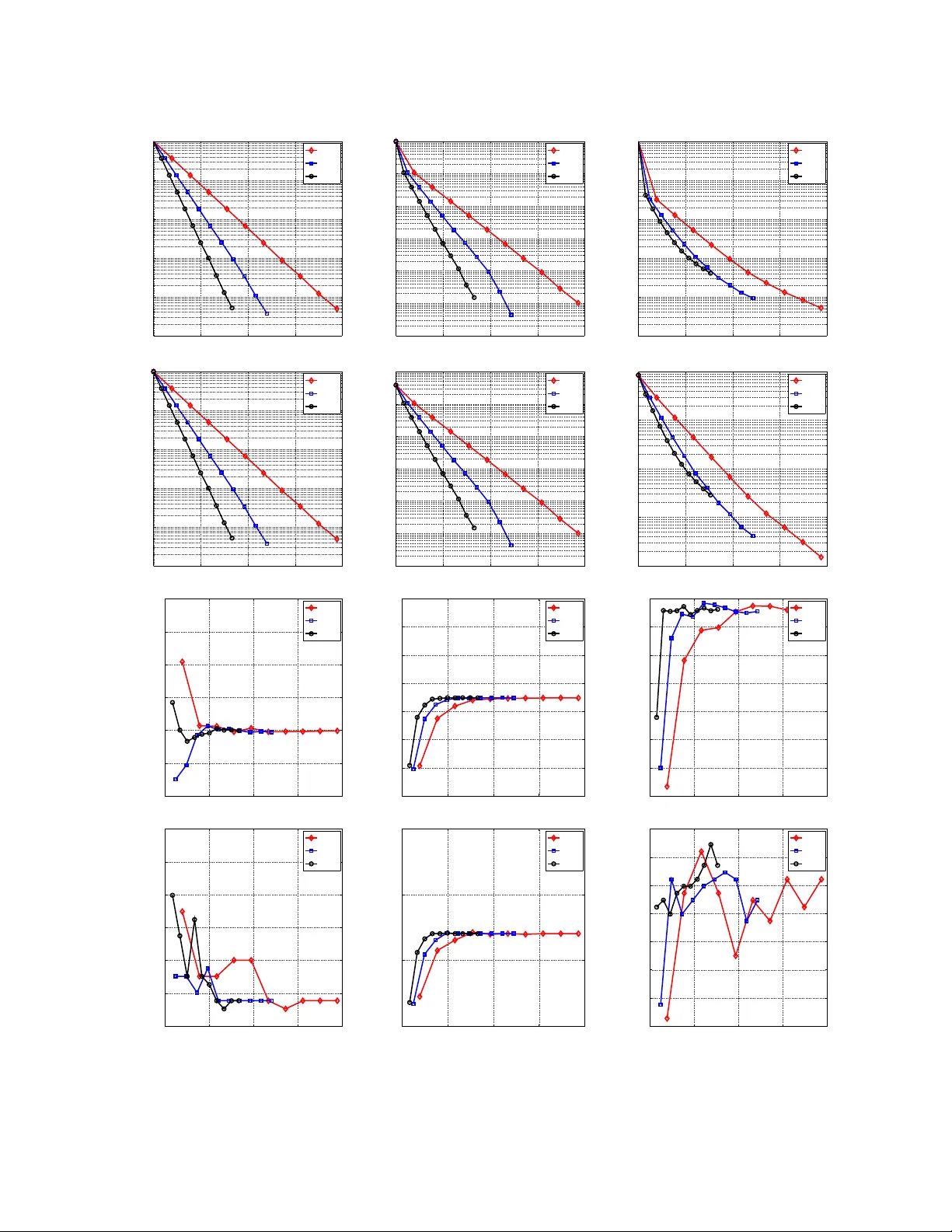
P arallel Co ordinate Descen t Metho ds for Big Data Optimization ∗ P eter Ric htárik Martin T ak áč Scho ol of Mathematics University of Edinbur gh Unite d Kingdom No vem ber 23, 2012 (revised No v ember 23, 2013) Abstract In this w ork we sho w that randomized (blo c k) co ordinate descen t metho ds can be accelerated b y parallelization when applied to the problem of minimizing the sum of a p artial ly sep ar able smo oth conv ex function and a simple separable con vex function. The theoretical sp eedup, as compared to the serial metho d, and referring to the n um b er of iterations needed to approximately solv e the problem with high probabilit y , is a simple expression dep ending on the num b er of parallel processors and a natural and easily computable measure of separabilit y of the smooth comp onen t of the ob jective function. In the w orst case, when no degree of separability is presen t, there ma y b e no sp eedup; in the b est case, when the problem is separable, the sp eedup is equal to the num ber of pro cessors. Our analysis also works in the mode when the num b er of blo c ks b eing up dated at each iteration is random, which allows for mo deling situations with busy or unreliable pro cessors. W e show that our algorithm is able to solv e a LASSO problem inv olving a matrix with 20 billion nonzeros in 2 hours on a large memory no de with 24 cores. Keyw ords: P arallel co ordinate descen t, big data optimization, partial separability , h uge- scale optimization, iteration complexit y , exp ected separable ov er-appro ximation, composite ob- jectiv e, con vex optimization, LASSO. 1 In tro duction Big data optimization. Recen tly there has b een a surge in interest in the design of algorithms suitable for solving conv ex optimization problems with a huge n umber of v ariables [16, 11]. Indeed, the size of problems arising in fields such as machine learning [1], net work analysis [29], PDEs [27], truss top ology design [15] and compressed sensing [5] usually grows with our capacit y to solve them, and is pro jected to gro w dramatically in the next decade. In fact, m uch of computational science ∗ This paper was a warded the 16th IMA Leslie F o x Prize in Numerical Analysis (2nd Prize; for M.T.) in June 2013. The w ork of the first author was supported by EPSR C grants EP/J020567/1 (Algorithms for Data Simplicit y) and EP/I017127/1 (Mathematics for V ast Digital Resources). The second author was supp orted by the Cen tre for Numerical Algorithms and Intelligen t Softw are (funded by EPSRC gran t EP/G036136/1 and the Scottish F unding Council). An op en source code with an efficient implemen tation of the algorithm(s) developed in this pap er is published here: h ttp://co de.google.com/p/ac-dc/. 1 is curren tly facing the “big data” challenge, and this w ork is aimed at dev eloping optimization algorithms suitable for the task. Co ordinate descent metho ds. Coordinate descent metho ds (CDM) are one of the most suc- cessful classes of algorithms in the big data optimization domain. Broadly sp eaking, CDMs are based on the strategy of up dating a single co ordinate (or a single blo c k of co ordinates) of the v ector of v ariables at eac h iteration. This often drastically reduces memory requirements as well as the arithmetic complexit y of a single iteration, making the methods easily implemen table and scalable. In certain applications, a single iteration can amount to as few as 4 m ultiplications and additions only [15]! On the other hand, man y more iterations are necessary for conv ergence than it is usual for classical gradien t metho ds. Indeed, the n umber of iterations a CDM requires to solve a smooth con vex optimization problem is O ( n ˜ LR 2  ) , where  is the error tolerance, n is the n umber v ariables (or blo c ks of v ariables), ˜ L is the av erage of the Lipsc hitz constants of the gradien t of the ob jective function asso ciated with the v ariables (blocks of v ariables) and R is the distance from the starting iterate to the set of optimal solutions. On balance, as observ ed by n umerous authors, serial CDMs are muc h more efficient for big data optimization problems than most other competing approac hes, suc h as gradient methods [10, 15]. P arallelization. W e wish to p oint out that for truly h uge-scale problems it is absolutely necessary to p ar al lelize . This is in l ine with the rise and ever increasing av ailabilit y of high p erformance computing systems built around m ulti-core pro cessors, GPU-accelerators and computer clusters, the success of whic h is ro oted in massive parallelization. This simple observ ation, com bined with the remark able scalabilit y of serial CDMs, leads to our belief that the study of parallel co ordinate descen t metho ds (PCDMs) is a v ery timely topic. Researc h Idea. The work presented in this pap er was motiv ated by the desire to answer the follo wing question: Under what natur al and e asily verifiable structur al assumptions on the obje ctive function do es p ar al lelization of a c o or dinate desc ent metho d le ad to ac c eler ation? Our starting p oin t was the follo wing simple observ ation. Assume that w e wish to minimize a separable function F of n v ariables (i.e., a function that can b e written as a sum of n functions eac h of which dep ends on a single v ariable only). F or simplicity , in this though t exp erimen t, assume that there are no constrain ts. Clearly , the problem of minimizing F can b e trivially decomp osed in to n indep enden t univ ariate problems. Now, if w e hav e n pro cessors/threads/cores, each assigned with the task of solving one of these problems, the num b er of parallel iterations should not dep end on the dimension of the problem 1 . In other words, we get an n -times sp eedup compared to the situation with a single pro cessor only . Note that any parallel algorithm of this t yp e can b e viewed as a parallel co ordinate descent method. Hence, a PCDM with n pro cessors should b e n -times faster than a serial one. If τ pro cessors are used instead, where 1 ≤ τ ≤ n , one w ould exp ect a τ -times sp eedup. 1 F or simplicity , assume the distance from the starting p oint to the set of optimal solutions do es not dep end on the dimension. 2 By extension, one would p erhaps expect that optimization problems with ob jectiv e functions whic h are “close to b eing separable” w ould also b e amenable to acceleration by parallelization, where the acceleration factor τ would b e reduced with the reduction of the “degree of separability”. One of the main messages of this pap er is an affirmative answer to this. Moreov er, w e give explicit and simple form ulae for the sp eedup factors. As it turns out, and as we discuss later in this section, many real-w orld big data optimization problems are, quite naturally , “close to b eing separable”. W e b eliev e that this means that PCDMs is a very promising class of algorithms when it comes to solving structured big data optimization problems. Minimizing a partially separable comp osite ob jectiv e. In this pap er we study the problem minimize n F ( x ) def = f ( x ) + Ω( x ) o sub ject to x ∈ R N , (1) where f is a (blo c k) p artial ly sep ar able smo oth conv ex function and Ω is a simple (blo c k) separable con vex function. W e allo w Ω to hav e v alues in R ∪ {∞} , and for regularization purp oses we assume Ω is prop er and closed. While (1) is seemingly an unconstrained problem, Ω can b e chosen to mo del simple conv ex constraints on individual blo c ks of v ariables. Alternativ ely , this function can b e used to enforce a certain structure (e.g., sparsit y) in the solution. F or a more detailed account we refer the reader to [16]. F urther, w e assume that this problem has a minimum ( F ∗ > −∞ ). What we mean b y “smo othness” and “simplicity” will b e made precise in the next section. Let us now describ e the k ey concept of partial separabilit y . Let x ∈ R N b e decomp osed into n non-o verlapping blo c ks of v ariables x (1) , . . . , x ( n ) (this will b e made precise in Section 2). W e assume throughout the paper that f : R N → R is p artial ly sep ar able of de gr e e ω , i.e., that it can b e written in the form f ( x ) = X J ∈J f J ( x ) , (2) where J is a finite collection of nonempty subsets of [ n ] def = { 1 , 2 , . . . , n } (p ossibly con taining identical sets multiple times), f J are differentiable con vex functions suc h that f J dep ends on blo c ks x ( i ) for i ∈ J only , and | J | ≤ ω for all J ∈ J . (3) Clearly , 1 ≤ ω ≤ n . The PCDM algorithms we develop and analyze in this pap er only need to know ω , they do not need to know the decomp osition of f giving rise to this ω . Examples of partially separable functions. Man y ob jectiv e functions naturally encountered in the big data setting are partially separable. Here we give examples of three loss/ob jectiv e functions frequen tly used in the machine learning literature and also elsewhere. F or simplicity , we assume all blo c ks are of size 1 (i.e., N = n ). Let f ( x ) = m X j =1 L ( x, A j , y j ) , (4) where m is the num b er of examples, x ∈ R n is the vector of features, ( A j , y j ) ∈ R n × R are lab eled examples and L is one of the three loss functions listed in T able 1. Let A ∈ R m × n with row j equal 3 Square Loss 1 2 ( A T j x − y j ) 2 Logistic Loss log(1 + e − y j A T j x ) Hinge Square Loss 1 2 max { 0 , 1 − y j A T j x } 2 T able 1: Three examples of loss of functions to A T j . Often, eac h example dep ends on a few features only; the maxim um o v er all features is the degree of partial separability ω . More formally , note that the j -th function in the sum (4) in all cases dep ends on k A j k 0 co ordinates of x (the num b er of nonzeros in the j -th row of A ) and hence f is partially separable of degree ω = max j k A j k 0 . All three functions of T able 1 are smo oth (based on the definition of smo othness in the next section). W e refer the reader to [13] for more examples of interesting (but nonsmo oth) partially separable functions arising in graph cuts and matrix completion. Brief literature review. Sev eral pap ers were written recently studying the iteration complexity of serial CDMs of v arious flav ours and in v arious settings. W e will only pro vide a brief summary here, for a more detailed accoun t we refer the reader to [16]. Classical CDMs up date the co ordinates in a cyclic order; the first attempt at analyzing the complexit y of such a metho d is due to [21]. Sto c hastic/randomized CDMs, that is, metho ds where the coordinate to b e up dated is c hosen randomly , were first analyzed for quadratic ob jectiv es [24, 4], later indep enden tly generalized to L 1 -regularized problems [23] and smo oth blo c k-structured problems [10], and finally unified and refined in [19, 16]. The problems considered in the ab o ve pap ers are either unconstrained or hav e (blo c k) separable constraints. Recently , randomized CDMs w ere developed for problems with linearly coupled constraints [7, 8]. A greedy CDM for L 1 -regularized problems w as first analyzed in [15]; more work on this topic include [5, 2]. A CDM with inexact up dates was first prop osed and analyzed in [26]. Partially separable problems were indep enden tly studied in [13], where an async hronous parallel sto c hastic gradien t algorithm was developed to solve them. When writing this pap er, the authors w ere aw are only of the parallel CDM prop osed and ana- lyzed in [1]. Several pap ers on the topic app eared around the time this pap er was finalized or after [6, 28, 22, 22, 14]. F urther pap ers on v arious asp ects of the topic of parallel CDMs, building on the w ork in this pap er, include [25, 17, 3, 18]. Con tents . W e start in Section 2 by describing the blo c k structure of the problem, establishing notation and detailing assumptions. Subsequently we prop ose and comment in detail on t wo parallel co ordinate descen t metho ds. In Section 3 w e summarize the main contributions of this paper. In Section 4 w e deal with issues related to the selection of the blo cks to b e up dated in each iteration. It will in volv e the dev elopment of some elementary random set theor y . Sections 5-6 deal with 4 issues related to the computation of the up date to the selected blo cks and develop a theory of Exp ected Separable Overappro ximation (ESO), which is a nov el tool we prop ose for the analysis of our algorithms. In Section 7 we analyze the iteration complexit y of our metho ds and finally , Section 8 rep orts on promising computational results. F or instance, w e conduct an exp erimen t with a big data (cca 350GB) LASSO problem with a billion v ariables. W e are able to solv e the problem using one of our metho ds on a large memory machine with 24 cores in 2 hours, pushing the difference b et w een the ob jective v alue at the starting iterate and the optimal p oin t from 10 22 do wn to 10 − 14 . W e also conduct exp eriments on real data problems coming from mac hine learning. 2 P arallel Blo c k Co ordinate Descen t Metho ds In Section 2.1 we formalize the blo c k structure of the problem, establish notation 2 that will b e used in the rest of the pap er and list assumptions. In Section 2.2 we prop ose tw o parallel blo c k co ordinate descent metho ds and comment in some detail on the steps. 2.1 Blo c k structure, notation and assumptions Some elements of the setup describ ed in this section was initially used in the analysis of blo ck co or- dinate descen t metho ds b y Nesterov [10] (e.g., blo c k structure, weigh ted norms and blo c k Lipsc hitz constan ts). The blo c k structure of (1) is giv en by a decomposition of R N in to n subspaces as follo ws. Let U ∈ R N × N b e a column p ermutation 3 of the N × N identit y matrix and further let U = [ U 1 , U 2 , . . . , U n ] b e a decomp osition of U into n submatrices, with U i b eing of size N × N i , where P i N i = N . Prop osition 1 (Blo c k decomp osition 4 ) . Any ve ctor x ∈ R N c an b e written uniquely as x = n X i =1 U i x ( i ) , (5) wher e x ( i ) ∈ R N i . Mor e over, x ( i ) = U T i x . Pr o of. Noting that U U T = P i U i U T i is the N × N identit y matrix, we hav e x = P i U i U T i x . Let us no w show uniqueness. Assume that x = P i U i x ( i ) 1 = P i U i x ( i ) 2 , where x ( i ) 1 , x ( i ) 2 ∈ R N i . Since U T j U i = ( N j × N j iden tity matrix, if i = j, N j × N i zero matrix, otherwise, (6) for ev ery j w e get 0 = U T j ( x − x ) = U T j P i U i ( x ( i ) 1 − x ( i ) 2 ) = x ( j ) 1 − x ( j ) 2 . In view of the ab o ve prop osition, from now on we write x ( i ) def = U T i x ∈ R N i , and refer to x ( i ) as the i -th blo ck of x . The definition of partial separability in the introduction is with resp ect to these blo c ks. F or simplicit y , w e will sometimes write x = ( x (1) , . . . , x ( n ) ) . 2 T able 8 in the app endix summarizes some of the key notation used frequently in the pap er. 3 The reason why we work with a permutation of the identit y matrix, rather than with the identit y itself, as in [10], is to enable the blo c ks b eing formed by nonc onse cutive co ordinates of x . This wa y we establish notation which mak es it p ossible to work with (i.e., analyze the prop erties of ) multiple block decomp ositions, for the sake of pic king the b est one, sub ject to some criteria. Moreov er, in some applications the co ordinates of x hav e a natural ordering to which the natural or efficient blo c k structure does not corresp ond. 4 This is a straightforeard result; we do not claim any nov elty and include it solely for the b enefit of the reader. 5 Pro jection onto a set of blo c ks. F or S ⊂ [ n ] and x ∈ R N w e write x [ S ] def = X i ∈ S U i x ( i ) . (7) That is, given x ∈ R N , x [ S ] is the vector in R N whose blo c ks i ∈ S are iden tical to those of x , but whose other blo c ks are zero ed out. In view of Prop osition 1, w e can equiv alen tly define x [ S ] blo c k-b y-blo c k as follows ( x [ S ] ) ( i ) = ( x ( i ) , i ∈ S, 0 ( ∈ R N i ) , otherwise. (8) Inner pro ducts. The standard Euclidean inner product in spaces R N and R N i , i ∈ [ n ] , will be denoted b y h· , ·i . Letting x, y ∈ R N , the relationship b et w een these inner pro ducts is giv en by h x, y i (5) = h n X j =1 U j x ( j ) , n X i =1 U i y ( i ) i = n X j =1 n X i =1 h U T i U j x ( j ) , y ( i ) i (6) = n X i =1 h x ( i ) , y ( i ) i . F or any w ∈ R n and x, y ∈ R N w e further define h x, y i w def = n X i =1 w i h x ( i ) , y ( i ) i . (9) F or vectors z = ( z 1 , . . . , z n ) T ∈ R n and w = ( w 1 , . . . , w n ) T ∈ R n w e write w  z def = ( w 1 z 1 , . . . , w n z n ) T . Norms. Spaces R N i , i ∈ [ n ] , are equipped with a pair of conjugate norms: k t k ( i ) def = h B i t, t i 1 / 2 , where B i is an N i × N i p ositiv e definite matrix and k t k ∗ ( i ) def = max k s k ( i ) ≤ 1 h s, t i = h B − 1 i t, t i 1 / 2 , t ∈ R N i . F or w ∈ R n ++ , define a pair of conjugate norms in R N b y k x k w = " n X i =1 w i k x ( i ) k 2 ( i ) # 1 / 2 , k y k ∗ w def = max k x k w ≤ 1 h y , x i = " n X i =1 w − 1 i ( k y ( i ) k ∗ ( i ) ) 2 # 1 / 2 . (10) Note that these norms are induced b y the inner pro duct (9) and the matrices B 1 , . . . , B n . Often w e will use w = L def = ( L 1 , L 2 , . . . , L n ) T ∈ R n , where the constan ts L i are defined b elo w. Smo othness of f . W e assume throughout the pap er that the gradient of f is blo c k Lipschitz, uniformly in x , with p ositiv e constan ts L 1 , . . . , L n , i.e., that for all x ∈ R N , i ∈ [ n ] and t ∈ R N i , k∇ i f ( x + U i t ) − ∇ i f ( x ) k ∗ ( i ) ≤ L i k t k ( i ) , (11) where ∇ i f ( x ) def = ( ∇ f ( x )) ( i ) = U T i ∇ f ( x ) ∈ R N i . An imp ortan t consequence of (11) is the following standard inequalit y [9]: f ( x + U i t ) ≤ f ( x ) + h∇ i f ( x ) , t i + L i 2 k t k 2 ( i ) . (12) 6 Separabilit y of Ω . W e assume that 5 Ω : R N → R ∪ { + ∞} is (blo c k) separable, i.e., that it can b e decomp osed as follows: Ω( x ) = n X i =1 Ω i ( x ( i ) ) , (13) where the functions Ω i : R N i → R ∪ { + ∞} are conv ex and closed. Strong con vexit y . In one of our t wo complexity results (Theorem 20) we will assume that either f or Ω (or b oth) is strongly conv ex. A function φ : R N → R ∪ { + ∞} is strongly conv ex with resp ect to the norm k · k w with con vexit y parameter µ φ ( w ) ≥ 0 if for all x, y ∈ dom φ , φ ( y ) ≥ φ ( x ) + h φ 0 ( x ) , y − x i + µ φ ( w ) 2 k y − x k 2 w , (14) where φ 0 ( x ) is any subgradien t of φ at x . The case with µ φ ( w ) = 0 reduces to con vexit y . Strong con vexit y of F ma y come from f or Ω (or b oth); we write µ f ( w ) (resp. µ Ω ( w ) ) for the (strong) con vexit y parameter of f (resp. Ω ). It follows from (14) that µ F ( w ) ≥ µ f ( w ) + µ Ω ( w ) . (15) The following c haracterization of strong con v exity will b e useful. F or all x, y ∈ dom φ and λ ∈ [0 , 1] , φ ( λx + (1 − λ ) y ) ≤ λφ ( x ) + (1 − λ ) φ ( y ) − µ φ ( w ) λ (1 − λ ) 2 k x − y k 2 w . (16) It can b e shown using (12) and (14) that µ f ( w ) ≤ L i w i . 2.2 Algorithms In this pap er w e develop and study tw o generic parallel co ordinate descent metho ds. The main metho d is PCDM1; PCDM2 is its “regularized” version which explicitly enforces monotonicity . As w e will see, b oth of these metho ds come in many v ariations, dep ending on how Step 3 is p erformed. Algorithm 1 Parallel Co ordinate Descent Metho d 1 (PCDM1) 1: Cho ose initial p oin t x 0 ∈ R N 2: for k = 0 , 1 , 2 , . . . do 3: Randomly generate a set of blo c ks S k ⊆ { 1 , 2 , . . . , n } 4: x k +1 ← x k + ( h ( x k )) [ S k ] 5: end for Let us commen t on the individual steps of the tw o metho ds. Step 3. At the b eginning of iteration k w e pick a random set ( S k ) of blo c ks to b e up dated (in parallel) during that iteration. The set S k is a realization of a random set-v alued mapping ˆ S with v alues in 2 [ n ] or, more precisely , it the sets S k are iid random sets with the distribution of ˆ S . F or brevit y , in this pap er we refer to such a mapping b y the name sampling . W e limit our attention to 5 F or examples of separable and blo c k separable functions we refer the reader to [16]. F or instance, Ω( x ) = k x k 1 is separable and blo c k separable (used in sparse optimization); and Ω( x ) = P i k x ( i ) k , where the norms are standard Euclidean norms, is blo c k separable (used in group lasso). One can mo del blo c k constraints by setting Ω i ( x ( i ) ) = 0 for x ∈ X i , where X i is some closed conv ex set, and Ω i ( x ( i ) ) = + ∞ for x / ∈ X i . 7 Algorithm 2 Parallel Co ordinate Descent Metho d 2 (PCDM2) 1: Cho ose initial p oin t x 0 ∈ R N 2: for k = 0 , 1 , 2 , . . . do 3: Randomly generate a set of blo c ks S k ⊆ { 1 , 2 , . . . , n } 4: x k +1 ← x k + ( h ( x k )) [ S k ] 5: If F ( x k +1 ) > F ( x k ) , then x k +1 ← x k 6: end for uniform samplings, i.e., random sets ha ving the following prop ert y: P ( i ∈ ˆ S ) is indep enden t of i . That is, the probability that a blo ck gets selected is the same for all blo c ks. Although w e giv e an iteration complexit y result co vering all such samplings (pro vided that eac h blo ck has a chance to b e up dated, i.e., P ( i ∈ ˆ S ) > 0 ), there are in teresting subclasses of uniform samplings (such as doubly uniform and nono verlapping uniform samplings; see Section 4) for which we giv e b etter results. Step 4. F or x ∈ R N w e define 6 . h ( x ) def = arg min h ∈ R N H β ,w ( x, h ) , (17) where H β ,w ( x, h ) def = f ( x ) + h∇ f ( x ) , h i + β 2 k h k 2 w + Ω( x + h ) , (18) and β > 0 , w = ( w 1 , . . . , w n ) T ∈ R n ++ are parameters of the metho d that w e will comment on later. Note that in view of (5), (10) and (13), H β ,w ( x, · ) is blo c k separable; H β ,w ( x, h ) = f ( x ) + n X i =1 n h∇ i f ( x ) , h ( i ) i + β w i 2 k h ( i ) k 2 ( i ) + Ω i ( x ( i ) + h ( i ) ) o . Consequen tly , we hav e h ( x ) = ( h (1) ( x ) , · · · , h ( n ) ( x )) ∈ R N , where h ( i ) ( x ) = arg min t ∈ R N i {h∇ i f ( x ) , t i + β w i 2 k t k 2 ( i ) + Ω i ( x ( i ) + t ) } . W e mentioned in the in tro duction that b esides (blo c k) separability , we require Ω to b e “simple”. By this w e mean that the ab o ve optimization problem leading to h ( i ) ( x ) is “simple” (e.g., it has a closed-form solution). Recall from (8) that ( h ( x k )) [ S k ] is the vector in R N iden tical to h ( x k ) except for blo c ks i / ∈ S k , whic h are zero ed out. Hence, Step 4 of b oth metho ds can b e written as follows: In parallel for i ∈ S k do: x ( i ) k +1 ← x ( i ) k + h ( i ) ( x k ) . P arameters β and w dep end on f and ˆ S and stay constan t throughout the algorithm. W e are not ready y et to explain why the up date is computed via (17) and (18) b ecause w e need tec hnical to ols, which will b e dev elop ed in Section 4, to do so. Here it suffices to say that the parameters β and w come from a separable quadratic o verappro ximation of E [ f ( x + h [ ˆ S ] )] , viewed as a function of h ∈ R N . Since exp ectation is in volv ed, we refer to this b y the name Exp ected 6 A similar map was used in [10] (with Ω ≡ 0 and β = 1 ) and [16] (with β = 1 ) in the analysis of serial coordinate descen t metho ds in the smo oth and comp osite case, resp ectiv ely . In lo ose terms, the nov elty here is the introduction of the parameter β and in developing theory which describ es what v alue β should hav e. Maps of this type are known as comp osite gradien t mapping in the literature, and were introduced in [12] 8 Separable Overappro ximation (ESO). This nov el concept, developed in this pap er, is one of the main to ols of our complexity analysis. Section 5 motiv ates and formalizes the concept, answers the why question, and develops some basic ESO theory . Section 6 is devoted to the computation of β and w for partially separable f and v arious sp ecial classes of uniform samplings ˆ S . Typically we will ha ve w i = L i , while β will dep end on e asily c omputable prop erties of f and ˆ S . F or example, if ˆ S is chosen as a subset of [ n ] of cardinality τ , with eac h subset chosen with the same probability (we sa y that ˆ S is τ -nice) then, assuming n > 1 , w e ma y choose w = L and β = 1 + ( ω − 1)( τ − 1) n − 1 , where ω is the degree of partial separability of f . More generally , if ˆ S is an y uniform sampling with the prop ert y | ˆ S | = τ with probability 1, then we ma y choose w = L and β = min { ω , τ } . Note that in b oth cases w = L and that the latter β is alw ays larger than (or equal to) the former one. This means, as we will see in Section 7, that we can give b etter complexity results for the former, more sp ecialized, sampling. W e analyze sev eral more options for ˆ S than the t wo just describ ed, and compute parameters β and w that should be used with them (for a summary , see T able 4). Step 5. The reason wh y , b esides PCDM1, w e also consider PCDM2, is the follo wing: in some situations we are not able to analyze the iteration complexit y of PCDM1 (non-strongly-con vex F where monotonicit y of the metho d is not guaran teed b y other means than b y directly enforcing it b y inclusion of Step 5). Let us remark that this issue arises for general Ω only . It do es not exist for Ω = 0 , Ω( · ) = λ k · k 1 and for Ω enco ding simple constraints on individual blo cks; in these cases one do es not need to consider PCDM2. Even in the case of general Ω w e sometimes get monotonicity for free, in which case there is no need to enforce it. Let us stress, how ev er, that we do not recommend implemen ting PCDM2 as this w ould introduce to o m uch o verhead; in our exp erience PCDM1 works w ell even in cases when we can only analyze PCDM2. 3 Smmary of Con tributions In this section w e summarize the main contributions of this pap er (not in order of significance). 1. Problem generalit y . W e giv e the first complexit y analysis for p ar al lel coordinate descent metho ds for problem (1) in its full generality . 2. Complexit y . W e show theoretically (Section 7) and n umerically (Section 8) that PCDM accelerates on its serial counterpart for partially se parable problems. In particular, w e establish t wo complexity theorems giving low er b ounds on the num b er of iterations k sufficien t for one or b oth of the PCDM v ariants (for details, see the precise statements in Section 7) to pro duce a random iterate x k for which the problem is appro ximately solved with high probability , i.e., P ( F ( x k ) − F ∗ ≤  ) ≥ 1 − ρ . The results, summarized in T able 2, hold under the standard assumptions listed in Section 2.1 and the additional assumption that f , ˆ S , β and w satisfy the follo wing inequality for all x, h ∈ R N : E [ f ( x + h [ ˆ S ] )] ≤ f ( x ) + E [ | ˆ S | ] n  h∇ f ( x ) , h i + β 2 k h k 2 w  . (19) This inequality , which w e call Exp ected Separable Overappro ximation (ESO), is the main new theoretical to ol that w e dev elop in this pap er for the analysis of our metho ds (Sections 4-6 are dev oted to the developmen t of this theory). 9 Setting Complexit y Theorem Con vex f O  β n E [ | ˆ S | ] 1  log  1 ρ  19 Strongly con vex f µ f ( w ) + µ Ω ( w ) > 0 n E [ | ˆ S | ] β + µ Ω ( w ) µ f ( w )+ µ Ω ( w ) log  F ( x 0 ) − F ∗ ρ  20 T able 2: Summary of the main complexity results for PCDM established in this pap er. The main observ ation here is that as the a v erage num b er of block updates p er iteration increases (sa y , ˆ τ = E [ | ˆ S | ] ), enabled b y the utilization of more pro cessors, the leading term in the complexity estimate, n/ ˆ τ , decreases in prop ortion. Ho wev er, β will generally grow with ˆ τ , whic h has an adverse effect on the sp eedup. Much of the theory in this pap er go es tow ards pro ducing formulas for β (and w ), for partially separable f and v arious classes of uniform samplings ˆ S . Naturally , the ideal situation is when β do es not grow with ˆ τ at all, or if it only grows very slo wly . W e show that this is the case for partially separable functions f with small ω . F or instance, in the extreme case when f is separable ( ω = 1 ), w e ha ve β = 1 and w e obtain linear sp eedup in ˆ τ . As ω increases, so do es β , dep ending on the law gov erning ˆ S . F ormulas for β and ω for v arious samplings ˆ S are summarized in T able 4. 3. Algorithm unification. Dep ending on the c hoice of the blo c k structure (as implied b y the c hoice of n and the matrices U 1 , . . . , U n ) and the wa y blo c ks are selected at every iteration (as given by the choice of ˆ S ), our framework enco des a family of known and new algorithms 7 (see T able 3). Metho d P arameters Commen t Gradien t descent n = 1 [12] Serial random CDM N i = 1 for all i and P ( | ˆ S | = 1) = 1 [16] Serial blo c k random CDM N i ≥ 1 for all i and P ( | ˆ S | = 1) = 1 [16] P arallel random CDM P ( | ˆ S | > 1) > 0 NEW Distributed random CDM ˆ S is a distributed sampling [17] 8 T able 3: New and known gradient metho ds obtained as sp ecial cases of our general framework. In particular, PCDM is the first method whic h “con tinuously” in terp olates betw een serial co ordinate descent and gradient (b y manipulating n and/or E [ | ˆ S | ] ). 4. P artial separabilit y . W e give the first analysis of a co ordinate descent t yp e metho d dealing with a partially separable loss / ob jectiv e. In order to run the metho d, w e need to know the Lipschitz constants L i and the degree of partial separability ω . It is crucial that these quan tities are often easily computable/predictable in the h uge-scale setting. F or example, if 7 All the metho ds are in their proximal v ariants due to the inclusion of the term Ω in the ob jective. 10 f ( x ) = 1 2 k Ax − b k 2 and w e c ho ose all blo cks to b e of size 1 , then L i is equal to the squared Euclidean norm of the i -th column of A and ω is equal to the maximum num b er of nonzeros in a ro w of A . Many problems in the big data setting hav e small ω compared to n . 5. Choice of blo c ks. T o the best of our knowledge, existing randomized strategies for paralleling gradien t-type metho ds (e.g., [1]) assume that ˆ S (or an equiv alen t thereof, based on the method) is chosen as a subset of [ n ] of a fixed cardinalit y , uniformly at random. W e refer to such ˆ S b y the name nic e sampling in this pap er. W e relax this assumption and our treatmen t is hence m uch more general. In fact, we allow for ˆ S to b e any uniform sampling. It is p ossible to further consider nonuniform samplings 9 , but this is b ey ond the scop e of this pap er. In particular, as a sp ecial case, our metho d allows for a v ariable num b er of blo c ks to be up dated throughout the iterations (this is ac hieved by the introduction of doubly uniform samplings ). This may b e useful in some settings such as when the problem is b eing solved in parallel by τ unreliable pro cessors each of whic h computes its up date h ( i ) ( x k ) with probability p b and is busy/do wn with probability 1 − p b ( binomial sampling ). Uniform, doubly uniform, nice, binomial and other samplings are defined, and their prop erties studied, in Section 4. 6. ESO and formulas for β and w . In T able 4 w e list parameters β and w for which ESO inequalit y (19) holds. Each ro w corresp onds to a sp ecific sampling ˆ S (see Section 4 for the definitions). The last 5 samplings are sp ecial cases of one or more of the first three samplings. Details suc h as what is ν, γ and “monotonic” ESO are explained in appropriate sections later in the text. When a sp ecific sampling ˆ S is used in the algorithm to select blo c ks in each iteration, the corresponding parameters β and w are to b e used in the metho d for the computation of the up date (see (17) and (18)). sampling ˆ S E [ | ˆ S | ] β w ESO monotonic? F ollo ws from uniform E [ | ˆ S | ] 1 ν  L No Thm 12 nono verlapping uniform n l 1 γ  L Y es Thm 13 doubly uniform E [ | ˆ S | ] 1 + ( ω − 1)  E [ | ˆ S | 2 ] E [ | ˆ S | ] − 1  max(1 ,n − 1) L No Thm 15 τ -uniform τ min { ω , τ } L Y es Thm 12 τ -nice τ 1 + ( ω − 1)( τ − 1) max(1 ,n − 1) L No Thm 14/15 ( τ , p b ) -binomial τ p b 1 + p b ( ω − 1)( τ − 1) max(1 ,n − 1) L No Thm 15 serial 1 1 L Y es Thm 13/14/15 fully parallel n ω L Y es Thm 13/14/15 T able 4: V alues of parameters β and w for v arious samplings ˆ S . En route to pro ving the iteration complexity results for our algorithms, we develop a theory of deterministic and exp ected separable ov erappro ximation (Sections 5 and 6) which we b eliev e is of indep enden t interest, to o. F or instance, metho ds based on ESO can b e compared fav orably 9 Revision note: See [18]. 11 to the Diagonal Quadratic Appro ximation (DQA) approach used in the decomp osition of sto c hastic optimization programs [20]. 7. P arallelization sp eedup. Our complexit y results can b e used to deriv e theoretical p ar al- lelization sp e e dup factors . F or several v arian ts of our metho d, in case of a non-strongly conv ex ob jective, these are giv en in Section 7.1 (T able 5). F or instance, in the case when all blo ck are up dated at each iteration (we later refer to ˆ S ha ving this prop ert y by the name ful ly p ar al lel sampling), the sp eedup factor is equal to n ω . If the problem is separable ( ω = 1 ), the sp eedup is equal to n ; if the problem is not separable ( ω = n ), there may b e no sp eedup. F or strongly con vex F the situation is even b etter; the details are given in Section 7.2. 8. Relationship to existing results. T o the b est of our knowledge, there are just tw o pap ers analyzing a parallel co ordinate descen t algorithm for conv ex optimization problems[1, 6]. In the first pap er all blo cks are of size 1 , ˆ S corresp onds to what w e call in this pap er a τ -nic e sampling (i.e., all sets of τ co ordinates are updated at each iteration with equal probability) and hence their algorithm is somewhat comparable to one of the many v arian ts of our general metho d. While the analysis in [1] works for a restricted range of v alues of τ , our results hold for all τ ∈ [ n ] . Moreo v er, the authors consider a more restricted class of functions f and the sp ecial case Ω = λ k x k 1 , which is simpler to analyze. Lastly , the theoretical sp eedups obtained in [1], when compared to the serial CDM metho d, dep end on a quantit y σ that is hard to compute in big data settings (it inv olves the computation of an eigenv alue of a huge-scale matrix). Our sp eedups are expressed in terms of natural and easily computable quan tity: the degree ω of partial separability of f . In the setting considered b y [1], in which more structure is av ailable, it turns out that ω is an upp er b ound 10 on σ . Hence, we sho w that one can dev elop the theory in a more general setting, and that it is not necessary to compute σ (which ma y b e complicated in the big data setting). The parallel CDM metho d of the second pap er [6] only allo ws all blo c ks to b e up dated at each iteration. Unfortunately , the analysis (and the method) is to o coarse as it does not offer an y theoretical sp eedup when compared to its serial coun terpart. In the sp ecial case when only a single blo ck is up dated in eac h iteration, uniformly at random, our theoretical results sp ecialize to those established in [16]. 9. Computations. W e demonstrate that our method is able to solve a LASSO problem in volving a matrix with a billion columns and 2 billion ro ws on a large memory no de with 24 cores in 2 hours (Section 8), achieving a 20 × sp eedup compared to the serial v ariant and pushing the residual by more than 30 degrees of magnitude. While this is done on an artificial problem under ideal conditions (controlling for small ω ), large sp eedups are p ossible in real data with ω small relativ e to n . W e also p erform additional exp erimen ts on real data sets from machine learning (e.g., training linear SVMs) to illustrate that the predictions of our theory match realit y . 10. Co de. The open source co de with an efficient implementation of the algorithm(s) developed in this pap er is published here: http://code.go ogle.com/p/ac-dc/. 10 Revision note requested by a reviewer: In the time since this pap er was p osted to arXiv, a num b er of follow-up pap ers were written analyzing parallel co ordinate descent metho ds and establishing connections b et ween a discrete quan tity analogous to ω (degree of partial/Nesterov separabilit y) and a sp ectral quan tity analogous to σ (largest eigen v alue of a certain matrix), most notably [3, 17]. See also [25], which uses a sp ectral quan tity , which can b e directly compared to ω . 12 4 Blo c k Samplings In Step 3 of b oth PCDM1 and PCDM2 w e choose a random set of blo cks S k to b e up dated at the curren t iteration. F ormally , S k is a realization of a r andom set-value d mapping ˆ S with v alues in 2 [ n ] , the collection of subsets of [ n ] . F or brevit y , in this pap er we refer to ˆ S b y the name sampling . A sampling ˆ S is uniquely characterized by the probability mass function P ( S ) def = P ( ˆ S = S ) , S ⊆ [ n ]; (20) that is, b y assigning probabilities to all subsets of [ n ] . F urther, we let p = ( p 1 , . . . , p n ) T , where p i def = P ( i ∈ ˆ S ) . (21) In Section 4.1 we describ e those samplings for which we analyze our metho ds and in Section 4.2 we pro ve several tec hnical results, which will b e useful in the rest of the pap er. 4.1 Uniform, Doubly Uniform and Nono v erlapping Uniform Samplings A sampling is pr op er if p i > 0 for all blo c ks i . That is, from the p ersp ectiv e of PCDM, under a prop er sampling eac h blo c k gets up dated with a p ositiv e probability at each iteration. Clearly , PCDM can not con verge for a sampling that is not prop er. A sampling ˆ S is uniform if all blo c ks get updated with the same probabilit y , i.e., if p i = p j for all i, j . W e show in (33) that, necessarily , p i = E [ | ˆ S | ] n . F urther, we sa y ˆ S is nil if P ( ∅ ) = 1 . Note that a uniform sampling is prop er if and only if it is not nil. All our iteration complexity results in this pap er are for PCDM used with a prop er uniform sampling (see Theorems 19 and 20) for whic h we can compute β and w giving rise to an inequality (we w e call “exp ected separable ov erappro ximation”) of the form (43). W e derive suc h inequalities for all prop er uniform samplings (Theorem 12) as well as refined results for t wo sp ecial sub classes thereof: doubly uniform samplings (Theorem 15) and nonov erlapping uniform samplings (Theorem 13). W e will no w give the definitions: 1. Doubly Uniform (DU) samplings. A DU sampling is one whic h generates all sets of equal cardinalit y with equal probability . That is, P ( S 0 ) = P ( S 00 ) whenev er | S 0 | = | S 00 | . The name comes from the fact that this definition p ostulates a different uniformity prop ert y , “standard” uniformit y is a consequence. Indeed, let us show that a DU sampling is necessarily uniform. Let q j = P ( | ˆ S | = j ) for j = 0 , 1 , . . . , n and note that from the definition we know that whenev er S is of cardinality j , we hav e P ( S ) = q j /  n j  . Finally , using this we obtain p i = X S : i ∈ S P ( S ) = n X j =1 X S : i ∈ S | S | = j P ( S ) = n X j =1 X S : i ∈ S | S | = j q j ( n j ) = n X j =1 ( n − 1 j − 1 ) ( n j ) q j = 1 n n X j =1 q j j = E [ | ˆ S | ] n . It is clear that eac h DU sampling is uniquely characterized by the vector of probabilities q ; its densit y function is given by P ( S ) = q | S |  n | S |  , S ⊆ [ n ] . (22) 13 2. Nono verlapping Uniform (NU) samplings. A NU sampling is one which is uniform and whic h assigns p ositive probabilities only to sets forming a partition of [ n ] . Let S 1 , S 2 , . . . , S l b e a partition of [ n ] , with | S j | > 0 for all j . The density function of a NU sampling corresp onding to this partition is giv en by P ( S ) = ( 1 l , if S ∈ { S 1 , S 2 , . . . , S l } , 0 , otherwise. (23) Note that E [ | ˆ S | ] = n l . Let us no w describ e sev eral interesting sp ecial cases of DU and NU samplings: 3. Nice sampling. Fix 1 ≤ τ ≤ n . A τ -nice sampling is a DU sampling with q τ = 1 . Interpr etation: There are τ processors/threads/cores a v ailable. At the beginning of each iteration we c ho ose a set of blo c ks using a τ -nice sampling (i.e., each subset of τ blo c ks is c hosen with the same probability), and assign eac h blo c k to a dedicated pro cessor/thread/core. Pro cessor assigned with blo ck i would compute and apply the up date h ( i ) ( x k ) . This is the sampling w e use in our computational exp erimen ts. 4. Indep enden t sampling. Fix 1 ≤ τ ≤ n . A τ -indep enden t sampling is a DU sampling with q k = (  n k  c k , k = 1 , 2 , . . . , τ , 0 , k = τ + 1 , . . . , n, where c 1 =  1 n  τ and c k =  k n  τ − P k − 1 i =1  k i  c i for k ≥ 2 . Interpr etation: There are τ pro cessors/threads/cores av ailable. Each pro cessor chooses one of the n blo c ks, uniformly at random and indep enden tly of the other pro cessors. It turns out that the set ˆ S of blo c ks selected this wa y is DU with q as giv en ab o v e. Since in one parallel iteration of our metho ds each block in ˆ S is up dated exactly once, this means that if t wo or more pro cessors pic k the same blo c k, all but one will b e idle. On the other hand, this sampling can b e generated extremely easily and in parallel! F or τ  n this sampling is a go od (and fast) approximation of the τ -nice sampling. F or instance, for n = 10 3 and τ = 8 w e hav e q 8 = 0 . 9723 , q 7 = 0 . 0274 , q 6 = 0 . 0003 and q k ≈ 0 for k = 1 , . . . , 5 . 5. Binomial sampling. Fix 1 ≤ τ ≤ n and 0 < p b ≤ 1 . A ( τ , p b ) -binomial sampling is defined as a DU sampling with q k =  τ k  p k b (1 − p b ) k , k = 0 , 1 , . . . , τ . (24) Notice that E [ | ˆ S | ] = τ p b and E [ | ˆ S | 2 ] = τ p b (1 + τ p b − p b ) . Interpr etation: Consider the follo wing situation with indep endent e qual ly unr eliable pr o c essors . W e hav e τ pro cessors, each of which is at any given moment av ailable with probability p b and busy with probabilit y 1 − p b , indep enden tly of the av ailabilit y of the other pro cessors. Hence, the num b er of av ailable pro cessors (and hence blo c ks that can b e up dated in parallel) at each iteration is a binomial random v ariable with parameters τ and p b . That is, the num b er of a v ailable pro cessors is equal to k with probabilit y q k . 14 – Case 1 (explicit sele ction of blo cks): W e learn that k pro cessors are a v ailable at the b e ginning of each iteration. Subsequen tly , we c ho ose k blo c ks using a k -nice sampling and “assign one blo c k” to each of the k av ailable pro cessors. – Case 2 (implicit sele ction of blo cks): W e c ho ose τ blo c ks using a τ -nice sampling and assign one to eac h of the τ pro cessors (w e do not know which will b e av ailable at the b eginning of the iteration). With probability q k , k of these will send their up dates. It is easy to c heck that the resulting effective sampling of blo c ks is ( τ , p b ) -binomial. 6. Serial sampling. This is a DU sampling with q 1 = 1 . Also, this is a NU sampling with l = n and S j = { j } for j = 1 , 2 , . . . , l . That is, at eac h iteration w e up date a single blo c k, uniformly at random. This was studied in [16]. 7. F ully parallel sampling. This is a DU sampling with q n = 1 . Also, this is a NU sampling with l = 1 and S 1 = [ n ] . That is, at each iteration we up date all blocks. The following simple result says that the intersection betw een the class of DU and NU samplings is v ery thin. A sampling is called vacuous if P ( ∅ ) > 0 . Prop osition 2. Ther e ar e pr e cisely two nonvacuous samplings which ar e b oth DU and NU: i) the serial sampling and ii) the ful ly p ar al lel sampling. Pr o of. Assume ˆ S is non v acuous, NU and DU. Since ˆ S is non v acuous, P ( ˆ S = ∅ ) = 0 . Let S ⊂ [ n ] b e any set for whic h P ( ˆ S = S ) > 0 . If 1 < | S | < n , then there exists S 0 6 = S of the same cardinalit y as S having a nonempt y in tersection with S . Since ˆ S is doubly uniform, we m ust ha ve P ( ˆ S = S 0 ) = P ( ˆ S = S 0 ) > 0 . Ho w ever, this con tradicts the fact that ˆ S is non-ov erlapping. Hence, ˆ S can only generate sets of cardinalities 1 or n with p ositiv e probability , but not b oth. One option leads to the fully parallel sampling, the other one leads to the serial sampling. 4.2 T ec hnical results F or a given sampling ˆ S and i, j ∈ [ n ] w e let p ij def = P ( i ∈ ˆ S , j ∈ ˆ S ) = X S : { i,j }⊂ S P ( S ) . (25) The follo wing simple result has several consequences which will b e used throughout the pap er. Lemma 3 (Sum ov er a random index set) . L et ∅ 6 = J ⊂ [ n ] and ˆ S b e any sampling. If θ i , i ∈ [ n ] , and θ ij , for ( i, j ) ∈ [ n ] × [ n ] ar e r e al c onstants, then 11 E   X i ∈ J ∩ ˆ S θ i   = X i ∈ J p i θ i , E   X i ∈ J ∩ ˆ S θ i | | J ∩ ˆ S | = k   = X i ∈ J P ( i ∈ ˆ S | | J ∩ ˆ S | = k ) θ i , (26) 11 Sum ov er an empty index set will, for conv enience, b e defined to b e zero. 15 E   X i ∈ J ∩ ˆ S X j ∈ J ∩ ˆ S θ ij   = X i ∈ J X j ∈ J p ij θ ij . (27) Pr o of. W e prov e the first statement, pro of of the remaining statements is essentially identical: E   X i ∈ J ∩ ˆ S θ i   (20) = X S ⊂ [ n ] X i ∈ J ∩ S θ i ! P ( S ) = X i ∈ J X S : i ∈ S θ i P ( S ) = X i ∈ J θ i X S : i ∈ S P ( S ) = X i ∈ J p i θ i . The consequences are summarized in the next theorem and the discussion that follo ws. Theorem 4. L et ∅ 6 = J ⊂ [ n ] and ˆ S b e an arbitr ary sampling. F urther, let a, h ∈ R N , w ∈ R n + and let g b e a blo ck sep ar able function, i.e., g ( x ) = P i g i ( x ( i ) ) . Then E h | J ∩ ˆ S | i = X i ∈ J p i , (28) E h | J ∩ ˆ S | 2 i = X i ∈ J X j ∈ J p ij , (29) E h h a, h [ ˆ S ] i w i = h a, h i p  w , (30) E h k h [ ˆ S ] k 2 w i = k h k 2 p  w , (31) E h g ( x + h [ ˆ S ] ) i = n X i =1 h p i g i ( x ( i ) + h ( i ) ) + (1 − p i ) g i ( x ( i ) ) i . (32) Mor e over, the matrix P def = ( p ij ) is p ositive semidefinite. Pr o of. Noting that | J ∩ ˆ S | = P i ∈ J ∩ ˆ S 1 , | J ∩ ˆ S | 2 = ( P i ∈ J ∩ ˆ S 1) 2 = P i ∈ J ∩ ˆ S P j ∈ J ∩ ˆ S 1 , h a, h [ ˆ S ] i w = P i ∈ ˆ S w i h a ( i ) , h ( i ) i , k h [ ˆ S ] k 2 w = P i ∈ ˆ S w i k h ( i ) k 2 ( i ) and g ( x + h [ ˆ S ] ) = X i ∈ ˆ S g i ( x ( i ) + h ( i ) ) + X i / ∈ ˆ S g i ( x ( i ) ) = X i ∈ ˆ S g i ( x ( i ) + h ( i ) ) + n X i =1 g i ( x ( i ) ) − X i ∈ ˆ S g i ( x ( i ) ) , all fiv e identities follow directly by applying Lemma 3. Finally , for any θ = ( θ 1 , . . . , θ n ) T ∈ R n , θ T P θ = n X i =1 n X j =1 p ij θ i θ j (27) = E [( X i ∈ ˆ S θ i ) 2 ] ≥ 0 . The ab o ve results hold for arbitrary samplings. Let us sp ecialize them, in order of decreasing generalit y , to uniform, doubly uniform and nice samplings. • Uniform samplings. If ˆ S is uniform, then from (28) using J = [ n ] we get p i = E [ | ˆ S | ] n , i ∈ [ n ] . (33) 16 Plugging (33) into (28), (30), (31) and (32) yields E h | J ∩ ˆ S | i = | J | n E [ | ˆ S | ] , (34) E h h a, h [ ˆ S ] i w i = E [ | ˆ S | ] n h a, h i w , (35) E h k h [ ˆ S ] k 2 w i = E [ | ˆ S | ] n k h k 2 w , (36) E h g ( x + h [ ˆ S ] ) i = E [ | ˆ S | ] n g ( x + h ) +  1 − E [ | ˆ S | ] n  g ( x ) . (37) • Doubly uniform samplings. Consider the case n > 1 ; the case n = 1 is trivial. F or doubly uniform ˆ S , p ij is constan t for i 6 = j : p ij = E [ | ˆ S | 2 −| ˆ S | ] n ( n − 1) . (38) Indeed, this follo ws from p ij = n X k =1 P ( { i, j } ⊆ ˆ S | | ˆ S | = k ) P ( | ˆ S | = k ) = n X k =1 k ( k − 1) n ( n − 1) P ( | ˆ S | = k ) . Substituting (38) and (33) into (29) then gives E [ | J ∩ ˆ S | 2 ] = ( | J | 2 − | J | ) E [ | ˆ S | 2 −| ˆ S | ] n max { 1 ,n − 1 } + | J | | ˆ S | n . (39) • Nice samplings. Finally , if ˆ S is τ -nice (and τ 6 = 0 ), then E [ | ˆ S | ] = τ and E [ | ˆ S | 2 ] = τ 2 , whic h used in (39) giv es E [ | J ∩ ˆ S | 2 ] = | J | τ n  1 + ( | J |− 1)( τ − 1) max { 1 ,n − 1 }  . (40) Moreo ver, assume that P ( | J ∩ ˆ S | = k ) 6 = 0 (this happ ens precisely when 0 ≤ k ≤ | J | and k ≤ τ ≤ n − | J | + k ). Then for all i ∈ J , P ( i ∈ ˆ S | | J ∩ ˆ S | = k ) =  | J |− 1 k − 1  n −| J | τ − k   | J | k  n −| J | τ − k  = k | J | . Substituting this in to (26) yields E   X i ∈ J ∩ ˆ S θ i | | J ∩ ˆ S | = k   = k | J | X i ∈ J θ i . (41) 17 5 Exp ected Separable Overappro ximation Recall that given x k , in PCDM1 the next iterate is the random v ector x k +1 = x k + h [ ˆ S ] for a particular c hoice of h ∈ R N . F urther recall that in PCDM2, x k +1 = ( x k + h [ ˆ S ] , if F ( x k + h [ ˆ S ] ) ≤ F ( x k ) , x k , otherwise, again for a particular choice of h . While in Section 2 w e mentioned how h is computed, i.e., that h is the minimizer of H β ,w ( x, · ) (see (17) and (18)), w e did not explain why is h computed this wa y . The reason for this is that the to ols needed for this were not yet dev elop ed at that p oin t (as we will see, some results from Section 4 are needed). In this section we giv e an answer to this why question. Giv en x k ∈ R N , after one step of PCDM1 performed with up date h we get E [ F ( x k +1 ) | x k ] = E [ F ( x k + h [ ˆ S ] ) | x k ] . On the the other hand, after one step of PCDM2 we hav e E [ F ( x k +1 ) | x k ] = E [min { F ( x k + h [ ˆ S ] ) , F ( x k ) } | x k ] ≤ min { E [ F ( x k + h [ ˆ S ] ) | x k ] , F ( x k ) } . So, for b oth PCDM1 and PCDM2 the following estimate holds, E [ F ( x k +1 ) | x k ] ≤ E [ F ( x k + h [ ˆ S ] ) | x k ] . (42) A go od choice for h to b e used in the algorithms wo uld b e one minimizing the right hand side of inequalit y (42). At the same time, we would lik e the minimization pro cess to b e decomp osable so that the up dates h ( i ) , i ∈ ˆ S , could b e computed in parallel. Ho wev er, the problem of finding suc h h is intractable in general ev en if w e do not require parallelizabilit y . Instead, w e prop ose to construct/compute a “simple” separable ov erapproximation of the right-hand side of (42). Since the ov erapproximation will b e separable, parallelizabilit y is guaranteed; “simplicity” means that the up dates h ( i ) can b e computed easily (e.g., in closed form). F rom no w on w e replace, for simplicity and w.l.o.g., the random vector x k b y a fixed deterministic v ector x ∈ R N . W e can thus remo ve conditioning in (42) and instead study the quan tit y E [ F ( x + h [ ˆ S ] )] . F urther, fix h ∈ R N . Note that if we can find β > 0 and w ∈ R n ++ suc h that E h f  x + h [ ˆ S ] i ≤ f ( x ) + E [ | ˆ S | ] n  h∇ f ( x ) , h i + β 2 k h k 2 w  , (43) w e indeed find a simple separable ov erappro ximation of E [ F ( x + h [ ˆ S ] )] : E [ F ( x + h [ ˆ S ] )] (1) = E [ f ( x + h [ ˆ S ] ) + Ω( x + h [ ˆ S ] )] (43) , (37) ≤ f ( x ) + E [ | ˆ S | ] n  h∇ f ( x ) , h i + β 2 k h k 2 w  +  1 − E [ | ˆ S | ] n  Ω( x ) + E [ | ˆ S | ] n Ω( x + h ) =  1 − E [ | ˆ S | ] n  F ( x ) + E [ | ˆ S | ] n H β ,w ( x, h ) , (44) where w e recall from (18) that H β ,w ( x, h ) = f ( x ) + h∇ f ( x ) , h i + β 2 k h k 2 w + Ω( x + h ) . That is, (44) sa ys that the exp ected ob jective v alue after one parallel step of our metho ds, if blo c k i ∈ ˆ S is up dated by h ( i ) , is b ounded ab o ve by a con vex combination of F ( x ) and H β ,w ( x, h ) . The natural c hoice of h is to set h ( x ) = arg min h ∈ R N H β ,w ( x, h ) . (45) 18 Note that this is precisely the choice we mak e in our metho ds. Since H β ,w ( x, 0) = F ( x ) , b oth PCDM1 and PCDM2 are monotonic in exp ectation. The ab o v e discussion leads to the following definition. Definition 5 (Exp ected Separable Overappro ximation (ESO)) . Let β > 0 , w ∈ R n ++ and let ˆ S b e a prop er uniform sampling. W e say that f : R N → R admits a ( β , w ) -ESO with resp ect to ˆ S if inequalit y (43) holds for all x, h ∈ R N . F or simplicit y , w e write ( f , ˆ S ) ∼ E S O ( β , w ) . A few remarks: 1. Inflation. If ( f , ˆ S ) ∼ E S O ( β , w ) , then for β 0 ≥ β and w 0 ≥ w , ( f , ˆ S ) ∼ E S O ( β 0 , w 0 ) . 2. Resh uffling. Since for any c > 0 w e hav e k h k 2 cw = c k h k 2 w , one can “sh uffle” constan ts b et ween β and w as follows: ( f , ˆ S ) ∼ E S O ( cβ , w ) ⇔ ( f , ˆ S ) ∼ E S O ( β , cw ) , c > 0 . (46) 3. Strong conv exity . If ( f , ˆ S ) ∼ E S O ( β , w ) , then β ≥ µ f ( w ) . (47) Indeed, it suffices to take exp ectation in (14) with y replaced by x + h [ ˆ S ] and compare the resulting inequalit y with (43) (this gives β k h k 2 w ≥ µ f ( w ) k h k 2 w , whic h must hold for all h ). Recall that Step 5 of PCDM2 was introduced so as to explicitly enforce monotonicit y in to the metho d as in some situations, as we will see in Section 7, w e can only analyze a monotonic algo- rithm. How ever, sometimes ev en PCDM1 behav es monotonically (without enforcing this b ehavior externally as in PCDM2). The following definition captures this. Definition 6 (Monotonic ESO) . Assume ( f , ˆ S ) ∼ E S O ( β , w ) and let h ( x ) be as in (45). W e sa y that the ESO is monotonic if F ( x + ( h ( x )) [ ˆ S ] ) ≤ F ( x ) , with probability 1, for all x ∈ dom F . 5.1 Deterministic Separable Ov erapproximation (DSO) of Partially Separable F unctions The follo wing theorem will b e useful in deriving ESO for uniform samplings (Section 6.1) and nono verlapping uniform samplings (Section 6.2). It will also b e useful in establishing monotonicity of some ESOs (Theorems 12 and 13). Theorem 7 (DSO) . Assume f is p artial ly sep ar able (i.e., it c an b e written in the form (2) ). L etting Supp( h ) def = { i ∈ [ n ] : h ( i ) 6 = 0 } , for al l x, h ∈ R N we have f ( x + h ) ≤ f ( x ) + h∇ f ( x ) , h i + max J ∈J | J ∩ Supp( h ) | 2 k h k 2 L . (48) Pr o of. Let us fix x and define φ ( h ) def = f ( x + h ) − f ( x ) − h∇ f ( x ) , h i . Fixing h , w e need to sho w that φ ( h ) ≤ θ 2 k h k 2 L for θ = max J ∈J θ J , where θ J def = | J ∩ Supp( h ) | . One can define functions φ J in an analogous fashion from the constituen t functions f J , whic h satisfy φ ( h ) = X J ∈J φ J ( h ) , (49) 19 φ J (0) = 0 , J ∈ J . (50) Note that (12) can b e written as φ ( U i h ( i ) ) ≤ L i 2 k h ( i ) k 2 ( i ) , i = 1 , 2 , . . . , n. (51) No w, since φ J dep ends on the intersection of J and the supp ort of its argumen t only , we hav e φ ( h ) (49) = X J ∈J φ J ( h ) = X J ∈J φ J n X i =1 U i h ( i ) ! = X J ∈J φ J   X i ∈ J ∩ Supp( h ) U i h ( i )   . (52) The argument in the last expression can b e written as a con v ex com bination of 1 + θ J v ectors: the zero v ector (with weigh t θ − θ J θ ) and the θ J v ectors { θ U i h ( i ) : i ∈ J ∩ Supp( h ) } (with weigh ts 1 θ ): X i ∈ J ∩ Supp( h ) U i h ( i ) =  θ − θ J θ × 0  +   1 θ × X i ∈ J ∩ Supp( h ) θ U i h ( i )   . (53) Finally , we plug (53) into (52) and use conv exit y and some simple algebra: φ ( h ) ≤ X J ∈J   θ − θ J θ φ J (0) + 1 θ X i ∈ J ∩ Supp( h ) φ J ( θ U i h ( i ) )   (50) = 1 θ X J ∈J X i ∈ J ∩ Supp( h ) φ J ( θ U i h ( i ) ) = 1 θ X J ∈J n X i =1 φ J ( θ U i h ( i ) ) = 1 θ n X i =1 X J ∈J φ J ( θ U i h ( i ) ) (49) = 1 θ n X i =1 φ ( θ U i h ( i ) ) (51) ≤ 1 θ n X i =1 L i 2 k θ h ( i ) k 2 ( i ) = θ 2 k h k 2 L . Besides the usefulness of the ab o ve result in deriving ESO inequalities, it is interesting on its o wn for the following reasons. 1. Blo c k Lipschitz con tinuit y of ∇ f . The DSO inequalit y (48) is a generalization of (12) since (12) can b e recov ered from (48) by c ho osing h with Supp( h ) = { i } for i ∈ [ n ] . 2. Global Lipsc hitz contin uit y of ∇ f . The DSO inequality also sa ys that the gradient of f is Lipsc hitz with Lipschitz constant ω with resp ect to the norm k · k L : f ( x + h ) ≤ f ( x ) + h∇ f ( x ) , h i + ω 2 k h k 2 L . (54) Indeed, this follo ws from (48) via max J ∈J | J ∩ Supp( h ) | ≤ max J ∈J | J | = ω . F or ω = n this has b een shown in [10]; our result for partially separable functions app ears to b e new. 3. Tigh tness of the global Lipsc hitz constant. The Lipschitz constan t ω is “tigh t” in the follo wing sense: there are functions for whic h ω cannot b e replaced in (54) b y any smaller n umber. W e will show this on a simple example. Let f ( x ) = 1 2 k Ax k 2 with A ∈ R m × n (blo c ks are of size 1). Note that we can write f ( x + h ) = f ( x ) + h∇ f ( x ) , h i + 1 2 h T A T Ah , and that L = ( L 1 , . . . , L n ) = diag ( A T A ) . Let D = Diag ( L ) . W e need to argue that there exists A for 20 whic h σ def = max h 6 =0 h T A T Ah k h k 2 L = ω . Since we know that σ ≤ ω (otherwise (54) would not hold), all w e need to show is that there is A and h for which h T A T Ah = ω h T D h. (55) Since f ( x ) = P m i =1 ( A T j x ) 2 , where A j is the j -th row of A , we assume that eac h ro w of A has at most ω nonzeros (i.e., f is partially separable of degree ω ). Let us pick A with the follo wing further prop erties: a) A is a 0-1 matrix, b) all rows of A ha v e exactly ω ones, c) all columns of A hav e exactly the same n umber ( k ) of ones. Immediate consequences: L i = k for all i , D = k I n and ω m = k n . If we let e m b e the m × 1 v ector of all ones and e n b e the n × 1 v ector of all ones, and set h = k − 1 / 2 e n , then h T A T Ah = 1 k e T n A T Ae n = 1 k ( ω e m ) T ( ω e m ) = ω 2 m k = ω n = ω 1 k e T n k I n e n = ω h T D h, establishing (55). Using similar techniques one can easily pro ve the follo wing more general result: Tigh tness also o ccurs for matrices A which in each row con tain ω identical nonzero elemen ts (but which can v ary from row to row). 5.2 ESO for a conv ex com bination of samplings Let ˆ S 1 , ˆ S 2 , . . . , ˆ S m b e a collection of samplings and let q ∈ R m b e a probability vector. By P j q j ˆ S j w e denote the sampling ˆ S given by P  ˆ S = S  = m X j =1 q j P ( ˆ S j = S ) . (56) This pro cedure allows us to build new samplings from existing ones. A natural interpretation of ˆ S is that it arises from a tw o stage pro cess as follo ws. Generating a set via ˆ S is equiv alent to first c ho osing j with probability q j , and then generating a set via ˆ S j . Lemma 8. L et ˆ S 1 , ˆ S 2 , . . . , ˆ S m b e arbitr ary samplings, q ∈ R m a pr ob ability ve ctor and κ : 2 [ n ] → R any function mapping subsets of [ n ] to r e als. If we let ˆ S = P j q j ˆ S j , then (i) E [ κ ( ˆ S )] = P m j =1 q j E [ κ ( ˆ S j )] , (ii) E [ | ˆ S | ] = P m j =1 q j E [ | ˆ S j | ] , (iii) P ( i ∈ ˆ S ) = P m j =1 q j P ( i ∈ ˆ S j ) , for any i = 1 , 2 , . . . , n , (iv) If ˆ S 1 , . . . , ˆ S m ar e uniform (r esp. doubly uniform), so is ˆ S . Pr o of. Statemen t (i) follows by writing E [ κ ( ˆ S )] as X S P ( ˆ S = S ) κ ( S ) (56) = X S m X j =1 q j P ( ˆ S j = S ) κ ( S ) = m X j =1 q j X S P ( ˆ S j = S ) κ ( S ) = m X j =1 q j E [ κ ( ˆ S j )] . Statemen t (ii) follows from (i) b y choosing κ ( S ) = | S | , and (iii) follo ws from (i) by c ho osing κ as follo ws: κ ( S ) = 1 if i ∈ S and κ ( S ) = 0 otherwise. Finally , if the samplings ˆ S j are uniform, from 21 (33) we kno w that P ( i ∈ ˆ S j ) = E [ | ˆ S j | ] /n for all i and j . Plugging this into identit y (iii) sho ws that P ( i ∈ ˆ S ) is independent of i , whic h shows that ˆ S is uniform. Now assume that ˆ S j are doubly uniform. Fixing arbitrary τ ∈ { 0 } ∪ [ n ] , for every S ⊂ [ n ] such that | S | = τ we hav e P ( ˆ S = S ) (56) = m X j =1 q j P ( ˆ S j = S ) = m X j =1 q j P ( | ˆ S j | = τ )  n τ  . As the last expression dep ends on S via | S | only , ˆ S is doubly uniform. Remarks: 1. If w e fix S ⊂ [ n ] and define k ( S 0 ) = 1 if S 0 = S and k ( S 0 ) = 0 otherwise, then statement (i) of Lemma8 reduces to (56). 2. All samplings arise as a combination of elementary samplings, i.e., samplings whose all weigh t is on one set only . Indeed, let ˆ S b e an arbitrary sampling. F or all subsets S j of [ n ] define ˆ S j b y P ( ˆ S j = S j ) = 1 and let q j = P ( ˆ S = S j ) . Then clearly , ˆ S = P j q j ˆ S j . 3. All doubly uniform samplings arise as con vex combinations of nice samplings. Often it is easier to establish ESO for a simple class of samplings (e.g., nice samplings) and then use it to obtain an ESO for a more complicated class (e.g., doubly uniform samplings as they arise as con vex combinations of nice samplings). The follo wing result is helpful in this regard. Theorem 9 (Conv ex Combination of Uniform Samplings) . L et ˆ S 1 , . . . , ˆ S m b e uniform samplings satisfying ( f , ˆ S j ) ∼ E S O ( β j , w j ) and let q ∈ R m b e a pr ob ability ve ctor. If P j q j ˆ S j is not nil, then   f , m X j =1 q j ˆ S j   ∼ E S O   1 P m j =1 q j E [ | ˆ S j | ] , m X j =1 q j E [ | ˆ S j | ] β j w j   . Pr o of. First note that from part (iv) of Lemma 8 w e kno w that ˆ S def = P j q j ˆ S j is uniform and hence it mak es sense to sp eak ab out ESO inv olving this sampling. Next, we can write E h f ( x + h [ ˆ S ] ) i = X S P ( ˆ S = S ) f ( x + h [ S ] ) (56) = X S X j q j P ( ˆ S j = S ) f ( x + h [ S ] ) = X j q j X S P ( ˆ S j = S ) f ( x + h [ S ] ) = X j q j E h f ( x + h [ ˆ S j ] ) i . It no w remains to use (43) and part (ii) of Lemma 8: m X j =1 q j E h f ( x + h [ ˆ S j ] ) i (43) ≤ m X j =1 q j  f ( x ) + E [ | ˆ S j | ] n  h∇ f ( x ) , h i + β j 2 k h k 2 w j  = f ( x ) + P j q j E [ | ˆ S j | ] n h∇ f ( x ) , h i + 1 2 n X j q j E [ | ˆ S j | ] β j k h k 2 w j ( Lemma 8 (ii) ) = f ( x ) + E [ | ˆ S | ] n  h∇ f ( x ) , h i + P j q j E [ | ˆ S j | ] β j k h k 2 w j 2 P j q j E [ | ˆ S j | ]  = f ( x ) + E [ | ˆ S | ] n  h∇ f ( x ) , h i + 1 2 P j q j E [ | ˆ S j | ] k h k 2 w  , 22 where w = P j q j E [ | ˆ S j | ] β j w j . In the third step we hav e also used the fact that E [ | ˆ S | ] > 0 whic h follo ws from the assumption that ˆ S is not nil. 5.3 ESO for a conic com bination of functions W e no w establish an ESO for a conic combination of functions each of whic h is already equipp ed with an ESO. It offers a complemen tary result to Theorem 9. Theorem 10 (Conic Com bination of F unctions) . If ( f j , ˆ S ) ∼ E S O ( β j , w j ) for j = 1 , . . . , m , then for any c 1 , . . . , c m ≥ 0 we have   m X j =1 c j f j , ˆ S   ∼ E S O   1 , m X j =1 c j β j w j   . Pr o of. Letting f = P j c j f j , w e get E   X j c j f j  x + h [ ˆ S ]    = X j c j E h f j  x + h [ ˆ S ] i ≤ X j c j  f j ( x ) + E [ | ˆ S | ] n  h∇ f j ( x ) , h i + β j 2 k h k 2 w j  = X j c j f j ( x ) + E [ | ˆ S | ] n   X j c j h∇ f j ( x ) , h i + X j c j β j 2 k h k 2 w j   = f ( x ) + E [ | ˆ S | ] n  h∇ f ( x ) , h i + 1 2 k h k 2 P j c j β j w j  . 6 Exp ected Separable Ov erappro ximation (ESO) of P artially Sep- arable F unctions Here we derive ESO inequalities for partially separable smo oth functions f and (prop er) uniform (Section 6.1), nonov erlapping uniform (Section 6.2), nice (Section 6.3) and doubly uniform (Sec- tion 6.4) samplings. 6.1 Uniform samplings Consider an arbitrary prop er sampling ˆ S and let ν = ( ν 1 , . . . , ν n ) T b e defined by ν i def = E h min { ω , | ˆ S |} | i ∈ ˆ S i = 1 p i X S : i ∈ S P ( S ) min { ω , | S |} , i ∈ [ n ] . Lemma 11. If ˆ S is pr op er, then E h f ( x + h [ ˆ S ] ) i ≤ f ( x ) + h∇ f ( x ) , h i p + 1 2 k h k 2 p  ν  L . (57) 23 Pr o of. Let us use Theorem 7 with h replaced b y h [ ˆ S ] . Note that max J ∈J | J ∩ Supp( h [ ˆ S ] ) | ≤ max J ∈J | J ∩ ˆ S | ≤ min { ω , | ˆ S |} . T aking exp ectations of b oth sides of (48) we therefore get E h f ( x + h [ ˆ S ] ) i (48) ≤ f ( x ) + E h h∇ f ( x ) , h [ ˆ S ] i i + 1 2 E h min { ω , | ˆ S |}k h [ ˆ S ] k 2 L i (30) = f ( x ) + h∇ f ( x ) , h i p + 1 2 E h min { ω , | ˆ S |}k h [ ˆ S ] k 2 L i . (58) It remains to b ound the last term in the expression ab o ve. Letting θ i = L i k h ( i ) k 2 ( i ) , w e hav e E h min { ω , | ˆ S |}k h [ ˆ S ] k 2 L i = E   X i ∈ ˆ S min { ω , | ˆ S |} L i k h ( i ) k 2 ( i )   = X S ⊂ [ n ] P ( S ) X i ∈ S min { ω , | S |} θ i = n X i =1 θ i X S : i ∈ S min { ω , | S |} P ( S ) = n X i =1 θ i p i E h min { ω , | ˆ S |} | i ∈ ˆ S i = n X i =1 θ i p i ν i = k h k 2 p  ν  L . (59) The ab o v e lemma will now b e used to establish ESO for arbitrary (prop er) uniform samplings. Theorem 12. If ˆ S is pr op er and uniform, then ( f , ˆ S ) ∼ E S O (1 , ν  L ) . (60) If, in addition, P ( | ˆ S | = τ ) = 1 (we say that ˆ S is τ -uniform), then ( f , ˆ S ) ∼ E S O (min { ω , τ } , L ) . (61) Mor e over, ESO (61) is monotonic. Pr o of. First, (60) follo ws from (57) since for a uniform sampling one has p i = E [ | ˆ S | ] /n for all i . If P ( | ˆ S | = τ ) = 1 , we get ν i = min { ω , τ } for all i ; (61) therefore follows from (60). Let us now establish monotonicit y . Using the deterministic separable ov erappro ximation (48) with h = h [ ˆ S ] , F ( x + h [ ˆ S ] ) ≤ f ( x ) + h∇ f ( x ) , h [ ˆ S ] i + max J ∈J | J ∩ ˆ S | 2 k h [ ˆ S ] k 2 L + Ω( x + h [ ˆ S ] ) ≤ f ( x ) + h∇ f ( x ) , h [ ˆ S ] i + β 2 k h [ ˆ S ] k 2 w + Ω( x + h [ ˆ S ] ) (62) = f ( x ) + X i ∈ ˆ S  h∇ f ( x ) , U i h ( i ) i + β w i 2 k h ( i ) k 2 ( i ) + Ω i ( x ( i ) + h ( i ) )  | {z } def = κ i ( h ( i ) ) + X i / ∈ ˆ S Ω i ( x ( i ) ) . (63) No w let h ( x ) = arg min h H β ,w ( x, h ) and recall that H β ,w ( x, h ) = f ( x ) + h∇ f ( x ) , h i + β 2 k h k 2 w + Ω( x + h ) = f ( x ) + n X i =1  h∇ f ( x ) , U i h ( i ) i + β w i 2 k h ( i ) k 2 ( i ) + Ω i ( x ( i ) + h ( i ) )  = f ( x ) + n X i =1 κ i ( h ( i ) ) . So, by definition, ( h ( x )) ( i ) minimizes κ i ( t ) and hence, ( h ( x )) [ ˆ S ] (recall (7)) minimizes the upp er b ound (63). In particular, ( h ( x )) [ ˆ S ] is b etter than a nil up date, whic h immediately gives F ( x + ( h ( x )) [ ˆ S ] ) ≤ f ( x ) + P i ∈ ˆ S κ i (0) + P i / ∈ ˆ S Ω i ( x ( i ) ) = F ( x ) . 24 Besides establishing an ESO result, we hav e just sho wn that, in the case of τ -uniform samplings with a conserv ativ e estimate for β , PCDM1 is monotonic, i.e., F ( x k +1 ) ≤ F ( x k ) . In particular, PCDM1 and PCDM2 coincide. W e call the estimate β = min { ω , τ } “conserv ative” b ecause it can b e improv ed (made smaller) in sp ecial cases; e.g., for the τ -nice sampling. Indeed, Theorem 14 establishes an ESO for the τ -nice sampling with the same w ( w = L ), but with β = 1 + ( ω − 1)( τ − 1) n − 1 , whic h is b etter (and can b e muc h b etter than) min { ω , τ } . Other things equal, smaller β directly translates in to b etter complexity . The price for the small β in the case of the τ -nice sampling is the loss of monotonicity . This is not a problem for strongly con vex ob jectiv e, but for merely con vex ob jective this is an issue as the analysis techniques we developed are only applicable to the monotonic metho d PCDM2 (see Theorem 19). 6.2 Nono v erlapping uniform samplings Let ˆ S b e a (prop er) nonov erlapping uniform sampling as defined in (23). If i ∈ S j , for some j ∈ { 1 , 2 , . . . , l } , define γ i def = max J ∈J | J ∩ S j | , (64) and let γ = ( γ 1 , . . . , γ n ) T . Note that, for example, if ˆ S is the serial uniform sampling, then l = n and S j = { j } for j = 1 , 2 , . . . , l , whence γ i = 1 for all i ∈ [ n ] . F or the fully parallel sampling we ha ve l = 1 and S 1 = { 1 , 2 , . . . , n } , whence γ i = ω for all i ∈ [ n ] . Theorem 13. If ˆ S a nonoverlapping uniform sampling, then ( f , ˆ S ) ∼ E S O (1 , γ  L ) . (65) Mor e over, this ESO is monotonic. Pr o of. By Theorem 7, used with h replaced b y h [ S j ] for j = 1 , 2 , . . . , l , we get f ( x + h [ S j ] ) ≤ f ( x ) + h∇ f ( x ) , h [ S j ] i + max J ∈J | J ∩ S j | 2 k h [ S j ] k 2 L . (66) Since ˆ S = S j with probabilit y 1 l , E h f ( x + h [ ˆ S ] ) i (66) ≤ 1 l l X j =1  f ( x ) + h∇ f ( x ) , h [ S j ] i + max J ∈J | J ∩ S j | 2 k h [ S j ] k 2 L  (64) = f ( x ) + 1 l   h∇ f ( x ) , h i + 1 2 l X j =1 X i ∈ S j γ i L i k h ( i ) k 2 ( i )   = f ( x ) + 1 l  h∇ f ( x ) , h i + 1 2 k h k 2 γ  L  , whic h establishes (65). It now only remains to establish monotonicit y . A dding Ω( x + h [ ˆ S ] ) to (66) with S j replaced by ˆ S , w e get F ( x + h [ ˆ S ] ) ≤ f ( x ) + h∇ f ( x ) , h [ ˆ S ] i + β 2 k h [ ˆ S ] k 2 w + Ω( x + h [ ˆ S ] ) . F rom this p oin t on the pro of is identical to that in Theorem 12, following equation (62). 25 6.3 Nice samplings In this section w e establish an ESO for nice samplings. Theorem 14. If ˆ S is the τ -nic e sampling and τ 6 = 0 , then ( f , ˆ S ) ∼ E S O  1 + ( ω − 1)( τ − 1) max(1 , n − 1) , L  . (67) Pr o of. Let us fix x and define φ and φ J as in the pro of of Theorem 7. Since E h φ ( h [ ˆ S ] ) i = E h f ( x + h [ ˆ S ] ) − f ( x ) − h∇ f ( x ) , h [ ˆ S ] i i (35) = E h f ( x + h [ ˆ S ] ) i − f ( x ) − τ n h∇ f ( x ) , h i , it no w only remains to show that E h φ ( h [ ˆ S ] ) i ≤ τ 2 n  1 + ( ω − 1)( τ − 1) max(1 ,n − 1)  k h k 2 L . (68) Let us now adopt the con ven tion that exp ectation conditional on an even t which happ ens with probabilit y 0 is equal to 0. Letting η J def = | J ∩ ˆ S | , and using this conv en tion, we can write E h φ ( h [ ˆ S ] ) i = X J ∈J E h φ J ( h [ ˆ S ] ) i = n X k =0 X J ∈J E h φ J ( h [ ˆ S ] ) | η J = k i P ( η J = k ) = n X k =0 P ( η J = k ) X J ∈J E h φ J ( h [ ˆ S ] ) | η J = k i . (69) Note that the last identit y follows if we assume, without loss of generality , that all sets J ha ve the same cardinalit y ω (this can b e ac hieved b y in tro ducing “dumm y” dep endencies). Indeed, in such a case P ( η J = k ) do es not dep end on J . No w, for any k ≥ 1 for which P ( η J = k ) > 0 (for some J and hence for all), using con vexit y of φ J , w e can now estimate E h φ J ( h [ ˆ S ] ) | η J = k i = E   φ J   1 k X i ∈ J ∩ ˆ S k U i h ( i )   | η J = k   ≤ E   1 k X i ∈ J ∩ ˆ S φ J  k U i h ( i )  | η J = k   (41) = 1 ω X i ∈ J φ J  k U i h ( i )  . (70) If w e now sum the inequalities (70) for all J ∈ J , we get X J ∈J E h φ J ( h [ ˆ S ] ) | η J = k i (70) ≤ 1 ω X J ∈J X i ∈ J φ J  k U i h ( i )  = 1 ω X J ∈J n X i =1 φ J  k U i h ( i )  = 1 ω n X i =1 X J ∈J φ J  k U i h ( i )  = 1 ω n X i =1 φ  k U i h ( i )  (51) ≤ 1 ω n X i =1 L i 2 k k h ( i ) k 2 ( i ) = k 2 2 ω k h k 2 L . (71) Finally , (68) follows after plugging (71) into (69): E h φ ( h [ ˆ S ] ) i ≤ X k P ( η J = k ) k 2 2 ω k h k 2 L = 1 2 ω k h k 2 L E [ | J ∩ ˆ S | 2 ] (40) = τ 2 n  1 + ( ω − 1)( τ − 1) max(1 ,n − 1)  k h k 2 L . 26 6.4 Doubly uniform samplings W e are now ready , using a b ootstrapping argumen t, to formulate and pro ve a result co vering all doubly uniform samplings. Theorem 15. If ˆ S is a (pr op er) doubly uniform sampling, then ( f , ˆ S ) ∼ E S O    1 + ( ω − 1)  E [ | ˆ S | 2 ] E [ | ˆ S | ] − 1  max(1 , n − 1) , L    . (72) Pr o of. Letting q k = P ( | ˆ S | = k ) and d = max { 1 , n − 1 } , we hav e E h f ( x + h [ ˆ S ] ) i = E h E h f ( x + h [ ˆ S ] ) | | ˆ S | ii = n X k =0 q k E h f ( x + h [ ˆ S ] ) | | ˆ S | = k i (67) ≤ n X k =0 q k h f ( x ) + k n  h∇ f ( x ) , h i + 1 2  1 + ( ω − 1)( k − 1) d  k h k 2 L i = f ( x ) + 1 n n X k =0 q k k h∇ f ( x ) , h i + 1 2 n n X k =1 q k  k  1 − ω − 1 d  + k 2 ω − 1 d  k h k 2 L = f ( x ) + E [ | ˆ S | ] n h∇ f ( x ) , h i + 1 2 n  E [ | ˆ S | ]  1 − ω − 1 d  + E [ | ˆ S | 2 ] ω − 1 d  k h k 2 L . This theorem could ha ve alternativ ely b een prov ed by writing ˆ S as a conv ex combination of nice samplings and applying Theorem 9. Note that Theorem 15 reduces to that of Theorem 14 in the sp ecial case of a nice sampling, and giv es the same result as Theorem 13 in the case of the serial and fully parallel samplings. 7 Iteration Complexit y In this section we prov e tw o iteration complexity theorems 12 . The first result (Theorem 19) is for non-strongly-con vex F and cov ers PCDM2 with no restrictions and PCDM1 only in the case when a monotonic ESO is used. The second result (Theorem 20) is for strongly conv ex F and co vers PCDM1 without an y monotonicity restrictions. Let us first establish t wo auxiliary results. Lemma 16. F or al l x ∈ dom F , H β ,w ( x, h ( x )) ≤ min y ∈ R N { F ( y ) + β − µ f ( w ) 2 k y − x k 2 w } . Pr o of. H β ,w ( x, h ( x )) (17) = min y ∈ R N H β ,w ( x, y − x ) = min y ∈ R N f ( x ) + h∇ f ( x ) , y − x i + Ω( y ) + β 2 k y − x k 2 w (14) ≤ min y ∈ R N f ( y ) − µ f ( w ) 2 k y − x k 2 w + Ω( y ) + β 2 k y − x k 2 w . 12 The developmen t is similar to that in [16] for the serial block coordinate descent metho d, in the comp osite case. Ho wev er, the results are v astly different. 27 Lemma 17. (i) L et x ∗ b e an optimal solution of (1) , x ∈ dom F and let R = k x − x ∗ k w . Then H β ,w ( x, h ( x )) − F ∗ ≤ (  1 − F ( x ) − F ∗ 2 β R 2  ( F ( x ) − F ∗ ) , if F ( x ) − F ∗ ≤ β R 2 , 1 2 β R 2 < 1 2 ( F ( x ) − F ∗ ) , otherwise. (73) (ii) If µ f ( w ) + µ Ω ( w ) > 0 and β ≥ µ f ( w ) , then for al l x ∈ dom F , H β ,w ( x, h ( x )) − F ∗ ≤ β − µ f ( w ) β + µ Ω ( w ) ( F ( x ) − F ∗ ) . (74) Pr o of. P art (i): Since we do not assume strong conv exity , we ha ve µ f ( w ) = 0 , and hence H β ,w ( x, h ( x )) ( Lemma 16 ) ≤ min y ∈ R N { F ( y ) + β 2 k y − x k 2 w } ≤ min λ ∈ [0 , 1] { F ( λx ∗ + (1 − λ ) x ) + β λ 2 2 k x − x ∗ k 2 w } ≤ min λ ∈ [0 , 1] { F ( x ) − λ ( F ( x ) − F ∗ ) + β λ 2 2 R 2 } . Minimizing the last expression in λ gives λ ∗ = min  1 , ( F ( x ) − F ∗ ) / ( β R 2 )  ; the result follo ws. Part (ii): Letting µ f = µ f ( w ) , µ Ω = µ Ω ( w ) and λ ∗ = ( µ f + µ Ω ) / ( β + µ Ω ) ≤ 1 , we hav e H β ,w ( x, h ( x )) ( Lemma 16 ) ≤ min y ∈ R N { F ( y ) + β − µ f 2 k y − x k 2 w } ≤ min λ ∈ [0 , 1] { F ( λx ∗ + (1 − λ ) x ) + ( β − µ f ) λ 2 2 k x − x ∗ k 2 w } (16) + (15) ≤ min λ ∈ [0 , 1] { λF ∗ + (1 − λ ) F ( x ) − ( µ f + µ Ω ) λ (1 − λ ) − ( β − µ f ) λ 2 2 k x − x ∗ k 2 w } ≤ F ( x ) − λ ∗ ( F ( x ) − F ∗ ) . The last inequalit y follows from the identit y ( µ f + µ Ω )(1 − λ ∗ ) − ( β − µ f ) λ ∗ = 0 . W e could hav e formulated part (ii) of the ab o ve result using the w eaker assumption µ F ( w ) > 0 , leading to a slightly stronger result. How ever, we prefer the ab o ve treatmen t as it giv es more insigh t. 7.1 Iteration complexity: con vex case The follo wing lemma will b e used to finish off the pro of of the complexity result of this section. Lemma 18 (Theorem 1 in [16]) . Fix x 0 ∈ R N and let { x k } k ≥ 0 b e a se quenc e of r andom ve ctors in R N with x k +1 dep ending on x k only. L et φ : R N → R b e a nonne gative function and define ξ k = φ ( x k ) . L astly, cho ose ac cur acy level 0 <  < ξ 0 , c onfidenc e level 0 < ρ < 1 , and assume that the se quenc e of r andom variables { ξ k } k ≥ 0 is nonincr e asing and has one of the fol lowing pr op erties: (i) E [ ξ k +1 | x k ] ≤ (1 − ξ k c 1 ) ξ k , for al l k , wher e c 1 >  is a c onstant, (ii) E [ ξ k +1 | x k ] ≤ (1 − 1 c 2 ) ξ k , for al l k such that ξ k ≥  , wher e c 2 > 1 is a c onstant. 28 If pr op erty (i) holds and we cho ose K ≥ 2 + c 1  (1 −  ξ 0 + log ( 1 ρ )) , or if pr op erty (ii) holds, and we cho ose K ≥ c 2 log( ξ 0 ρ ) , then P ( ξ K ≤  ) ≥ 1 − ρ . This lemma was recen tly extended in [26] so as to aid the analysis of a serial co ordinate descent metho d with inexact up dates, i.e., with h ( x ) c hosen as an appr oximate rather than exact minimizer of H 1 ,L ( x, · ) (see (17)). While in this pap er w e deal with exact up dates only , the results can b e extended to the inexact case. Theorem 19. Assume that ( f , ˆ S ) ∼ E S O ( β , w ) , wher e ˆ S is a pr op er uniform sampling, and let α = E [ | ˆ S | ] n . Cho ose x 0 ∈ dom F satisfying R w ( x 0 , x ∗ ) def = max x {k x − x ∗ k w : F ( x ) ≤ F ( x 0 ) } < + ∞ , (75) wher e x ∗ is an optimal p oint of (1) . F urther, cho ose tar get c onfidenc e level 0 < ρ < 1 , tar get ac cur acy level  > 0 and iter ation c ounter K in any of the fol lowing two ways: (i)  < F ( x 0 ) − F ∗ and K ≥ 2 + 2  β α  max n R 2 w ( x 0 , x ∗ ) , F ( x 0 ) − F ∗ β o   1 −  F ( x 0 ) − F ∗ + log  1 ρ  , (76) (ii)  < min { 2  β α  R 2 w ( x 0 , x ∗ ) , F ( x 0 ) − F ∗ } and K ≥ 2  β α  R 2 w ( x 0 , x ∗ )  log  F ( x 0 ) − F ∗ ρ  . (77) If { x k } , k ≥ 0 , ar e the r andom iter ates of PCDM (use PCDM1 if the ESO is monotonic, otherwise use PCDM2), then P ( F ( x K ) − F ∗ ≤  ) ≥ 1 − ρ . Pr o of. Since either PCDM2 is used (whic h is monotonic) or otherwise the ESO is monotonic, w e m ust hav e F ( x k ) ≤ F ( x 0 ) for all k . In particular, in view of (75) this implies that k x k − x ∗ k w ≤ R w ( x 0 , x ∗ ) . Letting ξ k = F ( x k ) − F ∗ , w e hav e E [ ξ k +1 | x k ] (44) ≤ (1 − α ) ξ k + α ( H β ,w ( x k , h ( x k )) − F ∗ ) (73) ≤ (1 − α ) ξ k + α max  1 − ξ k 2 β k x k − x ∗ k 2 w , 1 2  ξ k = max  1 − αξ k 2 β k x k − x ∗ k 2 w , 1 − α 2  ξ k ≤ max  1 − αξ k 2 β R 2 w ( x 0 , x ∗ ) , 1 − α 2  ξ k . (78) Consider case (i) and let c 1 = 2 β α max {R 2 w ( x 0 , x ∗ ) , ξ 0 β } . Contin uing with (78), we then get E [ ξ k +1 | x k ] ≤ (1 − ξ k c 1 ) ξ k for all k ≥ 0 . Since  < ξ 0 < c 1 , it suffices to apply Lemma 18(i). Consider now case (ii) and let c 2 = 2 β α R 2 w ( x 0 ,x ∗ )  . Observe now that whenever ξ k ≥  , from (78) w e get E [ ξ k +1 | x k ] ≤ (1 − 1 c 2 ) ξ k . By assumption, c 2 > 1 , and hence it remains to apply Lemma 18(ii). 29 The imp ortan t message of the ab o ve theorem is that the iteration complexity of our metho ds in the con vex case is O ( β α 1  ) . Note that for the serial metho d (PCDM1 used with ˆ S b eing the serial sampling) we hav e α = 1 n and β = 1 (see T able 4), and hence β α = n . It will b e interesting to study the p ar al lelization sp e e dup factor defined b y parallelization sp eedup factor = β α of the serial metho d β α of a parallel metho d = n β α of a parallel metho d . (79) T able 5, computed from the data in T able 4, giv es expressions for the parallelization sp eedup factors for PCDM based on a DU sampling (expressions for 4 sp ecial cases are given as well). ˆ S P arallelization sp eedup factor doubly uniform E [ | ˆ S | ] 1+ ( ω − 1) ( ( E [ | ˆ S | 2 ] / E [ | ˆ S | ]) − 1 ) max(1 ,n − 1) ( τ , p b ) -binomial τ 1 p b + ( ω − 1)( τ − 1) max(1 ,n − 1) τ -nice τ 1+ ( ω − 1)( τ − 1) max(1 ,n − 1) fully parallel n ω serial 1 T able 5: Conv ex F : Parallelization sp eedup factors for DU samplings. The factors below the line are sp ecial cases of the general expression. Maximum sp eedup is naturally obtained b y the fully parallel sampling: n ω . The sp eedup of the serial sampling (i.e., of the algorithm based on it) is 1 as w e are comparing it to itself. On the other end of the sp ectrum is the fully parallel sampling with a sp eedup of n ω . If the degree of partial separabilit y is small, then this factor will b e high — esp ecially so if n is h uge, which is the domain we are interested in. This pro vides an affirmative answer to the research question stated in italics in the in tro duction. Let us now lo ok at the sp eedup factor in the case of a τ -nice sampling. Letting r = ω − 1 max(1 ,n − 1) ∈ [0 , 1] (degree of partial separability normalized), the sp eedup factor can b e written as s ( r ) = τ 1 + r ( τ − 1) . Note that as long as r ≤ k − 1 τ − 1 ≈ k τ , the sp eedup factor will b e at least τ k . Also note that max { 1 , τ ω } ≤ s ( r ) ≤ min { τ , n ω } . Finally , if a sp eedup of at least s is desired, where s ∈ [0 , n ω ] , one needs to use at least 1 − r 1 /s − r pro cessors. F or illustration, in Figure 1 we plotted s ( r ) for a few v alues of τ . Note that for small v alues of τ , the sp eedup is significant and can b e as large as the num b er of pro cessors (in 30 the separable case). W e wish to stress that in man y applications ω will be a constan t indep enden t of n , whic h means that r will indeed b e very small in the huge-scale optimization setting. Figure 1: Parallelization sp eedup factor of PCDM1/PCDM2 used with τ -nice sampling as a function of the normalized/relativ e degree of partial separability r . 7.2 Iteration complexity: strongly conv ex case In this section we assume that F is strongly conv ex with resp ect to the norm k · k w and sho w that F ( x k ) con verges to F ∗ linearly , with high probability . Theorem 20. Assume F is str ongly c onvex with µ f ( w ) + µ Ω ( w ) > 0 . F urther, assume ( f , ˆ S ) ∼ E S O ( β , w ) , wher e ˆ S is a pr op er uniform sampling and let α = E [ | ˆ S | ] n . Cho ose initial p oint x 0 ∈ dom F , tar get c onfidenc e level 0 < ρ < 1 , tar get ac cur acy level 0 <  < F ( x 0 ) − F ∗ and K ≥ 1 α β + µ Ω ( w ) µ f ( w ) + µ Ω ( w ) log  F ( x 0 ) − F ∗ ρ  . (80) If { x k } ar e the r andom p oints gener ate d by PCDM1 or PCDM2, then P ( F ( x K ) − F ∗ ≤  ) ≥ 1 − ρ . Pr o of. Letting ξ k = F ( x k ) − F ∗ , w e hav e E [ ξ k +1 | x k ] (44) ≤ (1 − α ) ξ k + α ( H β ,w ( x k , h ( x k )) − F ∗ ) (74) ≤  1 − α µ f ( w )+ µ Ω ( w ) β + µ Ω ( w )  ξ k def = (1 − γ ) ξ k . Note that 0 < γ ≤ 1 since 0 < α ≤ 1 and β ≥ µ f ( w ) by (47). By taking exp ectation in x k , we obtain E [ ξ k ] ≤ (1 − γ ) k ξ 0 . Finally , it remains to use Marko v inequality: P ( ξ K >  ) ≤ E [ ξ K ]  ≤ (1 − γ ) K ξ 0  (80) ≤ ρ. 31 Instead of doing a direct calculation, w e could hav e finished the pro of of Theorem 20 b y applying Lemma 18(ii) to the inequality E [ ξ k +1 | x k ] ≤ (1 − γ ) ξ k . How ever, in order to b e able to use Lemma 18, we would hav e to first establish monotonicit y of the sequence { ξ k } , k ≥ 0 . This is not necessary using the direct approac h of Theorem 20. Hence, in the strongly conv ex case we can analyze PCDM1 and are not forced to resort to PCDM2. Consider now the following situations: 1. µ f ( w ) = 0 . Then the leading term in (80) is 1+ β /µ Ω ( w ) α . 2. µ Ω ( w ) = 0 . Then the leading term in (80) is β /µ f ( w ) α . 3. µ Ω ( w ) is “large enough”. Then β + µ Ω ( w ) µ f ( w )+ µ Ω ( w ) ≈ 1 and the leading term in (80) is 1 α . In a similar wa y as in the non-strongly conv ex case, define the parallelization sp eedup factor as the ratio of the leading term in (80) for the serial metho d (which has α = 1 n and β = 1 ) and the leading term for a parallel metho d: parallelization sp eedup factor = n 1+ µ Ω ( w ) µ f ( w )+ µ Ω ( w ) 1 α β + µ Ω ( w ) µ f ( w )+ µ Ω ( w ) = n β + µ Ω ( w ) α (1+ µ Ω ( w )) . (81) First, note that the sp eedup factor is indep endent of µ f . F urther, note that as µ Ω ( w ) → 0 , the sp eedup factor approaches the factor we obtained in the non-strongly conv ex case (see (79) and also T able 5). That is, for large v alues of µ Ω ( w ) , the sp eedup factor is approximately equal αn = E [ | ˆ S | ] , which is the av erage n umber of blo c ks up dated in a single parallel iteration. Note that th uis quantit y do es not dep end on the degree of partial separability of f . 8 Numerical Exp erimen ts In Section 8.1 w e present preliminary but very encouraging results showing that PCDM1 run on a system with 24 cores can solv e huge-scale partially-separable LASSO problems with a billion v ariables in 2 hours, compared with 41 hours on a single core. In Section 8.2 w e demonstrate that our analysis is in some sense tight. In particular, we sho w that the sp eedup predicted b y the theory can b e matched almost exactly by actual w all time sp eedup for a particular problem. 8.1 A LASSO problem with 1 billion v ariables In this exp erimen t w e solve a single randomly generated huge-scale LASSO instance, i.e., (1) with f ( x ) = 1 2 k Ax − b k 2 2 , Ω( x ) = k x k 1 , where A = [ a 1 , . . . , a n ] has 2 × 10 9 ro ws and N = n = 10 9 columns. W e generated the problem using a mo dified primal-dual generator [16] enabling us to choose the optimal solution x ∗ (and hence, indirectly , F ∗ ) and thus to con trol its cardinality k x ∗ k 0 , as well as the sparsit y level of A . In particular, we made the follo wing choices: k x ∗ k 0 = 10 5 , each column of A has exactly 20 nonzeros and the maxim um cardinalit y of a ro w of A is ω = 35 (the degree of partial separability of f ). The histogram of cardinalities is displa yed in Figure 2. W e solved the problem using PCDM1 with τ -nice sampling ˆ S , β = 1 + ( ω − 1)( τ − 1) n − 1 and w = L = ( k a 1 k 2 2 , · · · , k a n k 2 2 ) , for τ = 1 , 2 , 4 , 8 , 16 , 24 , on a single large-memory computer utilizing τ of its 24 32 0 5 10 15 20 25 30 35 0 0.5 1 1.5 2 2.5 3 x 10 8 cardinality count Figure 2: Histogram of the cardinalities of the rows of A . cores. The problem description took around 350GB of memory space. In fact, in our implementation w e departed from the just describ ed setup in tw o w ays. First, w e implemented an asynchr onous v ersion of the method; i.e., one in whic h cores do not wait for others to up date the curren t iterate within an iteration b efore reading x k +1 and pro ceeding to another up date step. Instead, eac h core reads the curren t iterate whenever it is ready with the previous up date step and applies the new up date as so on as it is computed. Second, as mentioned in Section 4, the τ -indep enden t sampling is for τ  n a v ery goo d approximation of the τ -nice sampling. W e therefore allo w ed eac h pro cessor to pic k a blo c k uniformly at random, indep enden tly from the other pro cessors. Choice of the first column of T able 6. In T able 6 we sho w the developmen t of the gap F ( x k ) − F ∗ as well as the elapsed time. The choice and meaning of the first column of the table, τ k n , needs some commentary . Note that exactly τ k coordinate up dates are p erformed after k iterations. Hence, the first column denotes the total n umber of co ordinate up dates normalized b y the n umber of co ordinates n . As an example, let τ 1 = 1 and τ 2 = 24 . Then if the serial metho d is run for k 1 = 24 iterations and the parallel one for k 2 = 1 iteration, b oth metho ds would hav e up dated the same num b er ( τ 1 k 1 = τ 2 k 2 = 24 ) of co ordinates; that is, they would “b e” in the same row of T able 6. In summary , each ro w of the table represen ts, in the sense describ ed ab o ve, the “same amount of w ork done” for each c hoice of τ . Progress to solving the problem. One can conjecture that the ab o ve meaning of the phrase “same amount of w ork done” w ould p erhaps b e roughly equiv alent to a different one: “same progress to solving the problem”. Indeed, it turns out, as can b e seen from the table and also from Fig- ure 3(a), that in each row for all algorithms the v alue of F ( x k ) − F ∗ is roughly of the same order of magnitude. This is not a trivial finding since, with increasing τ , older information is used to up date the co ordinates, and hence one would exp ect that conv ergence would b e slow er. It do es seem to b e slo wer—the gap F ( x k ) − F ∗ is generally higher if more pro cessors are used—but the slo wdown is limited. Lo oking at T able 6 and/or Figure 3(a), w e see that for all choices of τ , PCDM1 managed to push the gap b elo w 10 − 13 after 34 n to 37 n co ordinate up dates. The progress to solving the problem during the final 1 billion co ordinate up dates (i.e., when mo ving from the last-but-one to the last nonempt y line in each of the columns of T able 6 sho wing 33 F ( x k ) − F ∗ Elapsed Time τ k n τ = 1 τ = 2 τ = 4 τ = 8 τ = 16 τ = 24 τ = 1 τ = 2 τ = 4 τ = 8 τ = 16 τ = 24 0 6.27e+22 6.27e+22 6.27e+22 6.27e+22 6.27e+22 6.27e+22 0.00 0.00 0.00 0.00 0.00 0.00 1 2.24e+22 2.24e+22 2.24e+22 2.24e+22 2.24e+22 2.24e+22 0.89 0.43 0.22 0.11 0.06 0.05 2 2.24e+22 2.24e+22 2.24e+22 3.64e+19 2.24e+22 8.13e+18 1.97 1.06 0.52 0.27 0.14 0.10 3 1.15e+20 2.72e+19 8.37e+19 1.94e+19 1.37e+20 5.74e+18 3.20 1.68 0.82 0.43 0.21 0.16 4 5.25e+19 1.45e+19 2.22e+19 1.42e+18 8.19e+19 5.06e+18 4.28 2.28 1.13 0.58 0.29 0.22 5 1.59e+19 2.26e+18 1.13e+19 1.05e+17 3.37e+19 3.14e+18 5.37 2.91 1.44 0.73 0.37 0.28 6 1.97e+18 4.33e+16 1.11e+19 1.17e+16 1.33e+19 3.06e+18 6.64 3.53 1.75 0.89 0.45 0.34 7 2.40e+16 2.94e+16 7.81e+18 3.18e+15 8.39e+17 3.05e+18 7.87 4.15 2.06 1.04 0.53 0.39 8 5.13e+15 8.18e+15 6.06e+18 2.19e+14 5.81e+16 9.22e+15 9.15 4.78 2.37 1.20 0.61 0.45 9 8.90e+14 7.87e+15 2.09e+16 2.08e+13 2.24e+16 5.63e+15 10.43 5.39 2.67 1.35 0.69 0.51 10 5.81e+14 6.52e+14 7.75e+15 3.42e+12 2.89e+15 2.20e+13 11.73 6.02 2.98 1.51 0.77 0.57 11 5.13e+14 1.97e+13 2.55e+15 1.54e+12 2.55e+15 7.30e+12 12.81 6.64 3.29 1.66 0.84 0.63 12 5.04e+14 1.32e+13 1.84e+13 2.18e+11 2.12e+14 1.44e+12 14.08 7.26 3.60 1.83 0.92 0.68 13 2.18e+12 7.06e+11 6.31e+12 1.33e+10 1.98e+14 6.37e+11 15.35 7.88 3.91 1.99 1.00 0.74 14 7.77e+11 7.74e+10 3.10e+12 3.43e+09 1.89e+12 1.20e+10 16.65 8.50 4.21 2.14 1.08 0.80 15 1.80e+10 6.23e+10 1.63e+11 1.60e+09 5.29e+11 4.34e+09 17.94 9.12 4.52 2.30 1.16 0.86 16 1.38e+09 2.27e+09 7.86e+09 1.15e+09 1.46e+11 1.38e+09 19.23 9.74 4.83 2.45 1.24 0.91 17 3.63e+08 3.99e+08 3.07e+09 6.47e+08 2.92e+09 7.06e+08 20.49 10.36 5.14 2.61 1.32 0.97 18 2.10e+08 1.39e+08 2.76e+08 1.88e+08 1.17e+09 5.93e+08 21.76 10.98 5.44 2.76 1.39 1.03 19 3.81e+07 1.92e+07 7.47e+07 1.55e+06 6.51e+08 5.38e+08 23.06 11.60 5.75 2.91 1.47 1.09 20 1.27e+07 1.59e+07 2.93e+07 6.78e+05 5.49e+07 8.44e+06 24.34 12.22 6.06 3.07 1.55 1.15 21 4.69e+05 2.65e+05 8.87e+05 1.26e+05 3.84e+07 6.32e+06 25.42 12.84 6.36 3.22 1.63 1.21 22 1.47e+05 1.16e+05 1.83e+05 2.62e+04 3.09e+06 1.41e+05 26.64 13.46 6.67 3.38 1.71 1.26 23 5.98e+04 7.24e+03 7.94e+04 1.95e+04 5.19e+05 6.09e+04 27.92 14.08 6.98 3.53 1.79 1.32 24 3.34e+04 3.26e+03 5.61e+04 1.75e+04 3.03e+04 5.52e+04 29.21 14.70 7.28 3.68 1.86 1.38 25 3.19e+04 2.54e+03 2.17e+03 5.00e+03 6.43e+03 4.94e+04 30.43 15.32 7.58 3.84 1.94 1.44 26 3.49e+02 9.62e+01 1.57e+03 4.11e+01 3.68e+03 4.91e+04 31.71 15.94 7.89 3.99 2.02 1.49 27 1.92e+02 8.38e+01 6.23e+01 5.70e+00 7.77e+02 4.90e+04 33.00 16.56 8.20 4.14 2.10 1.55 28 1.07e+02 2.37e+01 2.38e+01 2.14e+00 6.69e+02 4.89e+04 34.23 17.18 8.49 4.30 2.17 1.61 29 6.18e+00 1.35e+00 1.52e+01 2.35e-01 3.64e+01 4.89e+04 35.31 17.80 8.79 4.45 2.25 1.67 30 4.31e+00 3.93e-01 6.25e-01 4.03e-02 2.74e+00 3.15e+01 36.60 18.43 9.09 4.60 2.33 1.73 31 6.17e-01 3.19e-01 1.24e-01 3.50e-02 6.20e-01 9.29e+00 37.90 19.05 9.39 4.75 2.41 1.78 32 1.83e-02 3.06e-01 3.25e-02 2.41e-03 2.34e-01 3.10e-01 39.17 19.67 9.69 4.91 2.48 1.84 33 3.80e-03 1.75e-03 1.55e-02 1.63e-03 1.57e-02 2.06e-02 40.39 20.27 9.99 5.06 2.56 1.90 34 7.28e-14 7.28e-14 1.52e-02 7.46e-14 1.20e-02 1.58e-02 41.47 20.89 10.28 5.21 2.64 1.96 35 - - 1.24e-02 - 1.23e-03 8.70e-14 - - 10.58 - 2.72 2.02 36 - - 2.70e-03 - 3.99e-04 - - - 10.88 - 2.80 - 37 - - 7.28e-14 - 7.46e-14 - - - 11.19 - 2.87 - T able 6: A LASSO problem with 10 9 v ariables solved by PCDM1 with τ = 1, 2, 4, 8, 16 and 24. F ( x k ) − F ∗ ) is remark able. The metho d managed to push the optimality gap by 9-12 degrees of magnitude. W e do not hav e an explanation for this phenomenon; we do not give lo cal conv ergence 34 0 10 20 30 40 10 −10 10 0 10 10 10 20 # coordinate updates normalized [(k τ )/n] F(x k )−F * 1 Core 2 Cores 4 Cores 8 Cores 16 Cores 24 Cores (a) F or each τ , PCDM1 needs roughly the same num b er of co ordinate up dates to solv e the problem. 0 10 20 30 40 10 −10 10 0 10 10 10 20 # iterations normalized [k/n] F(x k )−F * 1 Core 2 Cores 4 Cores 8 Cores 16 Cores 24 Cores (b) Doubling the n umber of cores corresponds to roughly halving the num b er of iterations. 0 10 20 30 40 50 10 −10 10 0 10 10 10 20 wall time [hours] F(x k )−F * 1 Core 2 Cores 4 Cores 8 Cores 16 Cores 24 Cores (c) Doubling the n umber of cores corresp onds to roughly halving the wall time. 0 10 20 30 40 0 5 10 15 20 25 # coordinate updates normalized [(k τ )/n] empirical speedup 1 Core 2 Cores 4 Cores 8 Cores 16 Cores 24 Cores (d) P arallelization sp eedup is essen tially equal to the n umber of cores. Figure 3: F our computational insigh ts into the workings of PCDM1. estimates in this pap er. It is certainly the case though that once the metho d managed to find the nonzero places of x ∗ , fast lo cal conv ergence comes in. P arallelization sp eedup. Since a parallel metho d utilizing τ cores manages to do the same n umber of co ordinate up dates as the serial one τ times faster, a direct consequence of the ab o ve observ ation is that doubling the num b er of cores corresp onds to roughly halving the num b er of iterations (see Figure 3(b). This is due to the fact that ω  n and τ  n . It turns out that the n umber of iterations is an excellen t predictor of w all time; this can b e seen b y comparing Figures 3(b) and 3(c). Finally , it follows from the ab o v e, and can b e seen in Figure 3(d), that the sp eedup of PCDM1 utilizing τ cores is roughly equal to τ . Note that this is caused by the fact that the problem is, relativ e to its dimension, partially separable to a very high degree. 35 8.2 Theory versus reality In our second experiment w e demonstrate n umerically that our parallelization sp eedup estimates are in some sense tight. F or this purp ose it is not necessary to reach for complicated problems and high dimensions; we hence minimize the function 1 2 k Ax − b k 2 2 with A ∈ R 3000 × 1000 . Matrix A w as generated so that its ev ery row con tains exactly ω non-zero v alues all of which are equal (recall the construction in p oin t 3 at the end of Section 5.1). 10 0 10 1 10 2 10 3 10 0 10 1 10 2 # of cores ( τ ) speedup ω =5 ω =10 ω =50 ω =100 Figure 4: Theoretical sp eedup factor predicts the actual sp eedup almost exactly for a carefully constructed problem. W e generated 4 matrices with ω = 5 , 10 , 50 and 100 and measured the num b er of iterations needed for PCDM1 used with τ -nice sampling to get within  = 10 − 6 of the optimal v alue. The exp erimen t w as done for a range of v alues of τ (b et w een 1 core and 1000 cores). The solid lines in Figure 4 presen t the the or etic al sp e e dup factor for the τ -nice sampling, as presen ted in T able 5. The markers in each case corresp ond to empiric al sp e e dup factor defined as # of iterations till  -solution is found b y PCDM1 used with serial sampling # of iterations till  -solution is found b y PCDM1 used with τ -nice sampling . As can b e seen in Figure 4, the match b et w een theoretical prediction and reality is remark able! A partial explanation of this phenomenon lies in the fact that w e hav e carefully designed the problem so as to ensure that the degree of partial separability is equal to the Lipschitz constan t σ of ∇ f (i.e., that it is not a gross ov erestimation of it; see Section 5.1). This fact is useful since it is p ossible to pro ve complexity results with ω replaced by σ . Ho wev er, this answ er is far from satisfying, and a deep er understanding of the phenomenon remains an op en problem. 8.3 T raining linear SVMs with bad data for PCDM In this exp erimen t w e test PCDM on the problem of training a linear Support V ector Machine (SVM) based on n lab eled training examples: ( y i , A i ) ∈ { +1 , − 1 } × R d , i = 1 , 2 , . . . , n . In particular, w e consider the primal problem of minimizing L2-regularized a verage hinge-loss, 36 min w ∈ R d ( g ( w ) def = 1 n n X i =1 [1 − y i h w , a i i ] + + λ 2 k w k 2 2 ) , and the dual problem of maximizing a conca ve quadratic sub ject to zero-one b o x constrain ts, max x ∈ R n , 0 ≤ x ( i ) ≤ 1 ( − f ( x ) def = − 1 2 λn 2 x T Z x + 1 n n X i =1 x ( i ) ) , where Z ∈ R n × n with Z ii = y i y j h A i , A j i . It is a standard practice to apply serial co ordinate descen t to the dual. Here we apply p ar al lel co ordinate descent (PCDM; with τ -nice sampling of co ordinates) to the dual; i.e., minimize the conv ex function f sub ject to b o x constraints. In this setting all blo c ks are of size N i = 1 . The dual can b e written in the form (1), i.e., min x ∈ R n { F ( x ) = f ( x ) + Ω( x ) } , where Ω( x ) = 0 whenev er x ( i ) ∈ [0 , 1] for all i = 1 , 2 , . . . , n , and Ω( x ) = + ∞ otherwise. W e consider the rcv1.binary dataset 13 . The training data has n = 677 , 399 examples, d = 47 , 236 features, 49 , 556 , 258 nonzero elemen ts and requires cca 1GB of RAM for storage. Hence, this is a small-scale problem. The degree of partial separability of f is ω = 291 , 516 (i.e., the maxim um num b er of examples sharing a giv en feature). This is a very large n umber relative to n , and hence our theory w ould predict rather bad b ehavior for PCDM. W e use PCDM1 with τ - nice sampling ( appro ximating it by τ -indep enden t sampling for added efficiency) with β follo wing Theorem 14: β = 1 + ( τ − 1)( ω − 1) n − 1 . The results of our exp erimen ts are summarized in Figure 5. Eac h column corresp onds to a differen t lev el of regularization: λ ∈ { 1 , 10 − 3 , 10 − 5 } . The ro ws sho w the 1) dualit y gap, 2) dual sub optimalit y , 3) train error and 4) test error; each for 1,4 and 16 pro cessors ( τ = 1 , 4 , 16 ). Observe that the plots in the first tw o ro ws are nearly iden tical; which means that the metho d is able to solv e the primal problem at ab out the same sp eed as it can solve the dual problem 14 . Observ e also that in all cases, duality gap of around 0 . 01 is sufficient for training as training error (classification p erformance of the SVM on the train data) do es not decrease further after this p oin t. Also observe the effect of λ on training accuracy: accuracy increases from ab out 92% for λ = 1 , through 95 . 3% for λ = 10 − 3 to ab o v e 97 . 8% with λ = 10 − 5 . In our case, c ho osing smaller λ do es not lead to ov erfitting; the test error on test dataset (# features =677,399, # examples = 20,242) increases as λ decreases, quickly reaching ab out 95% (after 2 seconds of training) for λ = 0 . 001 and for the smallest λ going b eyond 97% . Note that PCDM with τ = 16 is ab out 2.5 × faster than PCDM with τ = 1 . This is m uch less than linear sp eedup, but is fully in line with our theoretical predictions. Indeed, for τ = 16 w e get β = 7 . 46 . Consulting T able 5, we see that the theory sa ys that with τ = 16 pro cessors w e should exp ect the parallelization sp eedup to b e P S F = τ /β = 2 . 15 . 13 http://www.csie.ntu.edu.tw/~cjlin/libsvmtools/datasets/binary.html#rcv1.binary 14 Revision comment: W e did not prop ose primal-dual versions of PCDM in this pap er, but we do so in the follow up work [25]. In this pap er, for the SVM problem, our metho ds and theory apply to the dual only . 37 λ = 1 λ = 0 . 001 λ = 0 . 00001 0 2 4 6 8 10 −5 10 −4 10 −3 10 −2 10 −1 10 0 Compuat. time [sec.] Duality gap τ =1 τ =4 τ =16 0 2 4 6 8 10 −6 10 −5 10 −4 10 −3 10 −2 10 −1 10 0 Compuat. time [sec.] Duality gap τ =1 τ =4 τ =16 0 2 4 6 8 10 −5 10 −4 10 −3 10 −2 10 −1 10 0 Compuat. time [sec.] Duality gap τ =1 τ =4 τ =16 0 2 4 6 8 10 −5 10 −4 10 −3 10 −2 10 −1 10 0 Compuat. time [sec.] Dual suboptimality τ =1 τ =4 τ =16 0 2 4 6 8 10 −6 10 −5 10 −4 10 −3 10 −2 10 −1 10 0 Compuat. time [sec.] Dual suboptimality τ =1 τ =4 τ =16 0 2 4 6 8 10 −5 10 −4 10 −3 10 −2 10 −1 Compuat. time [sec.] Dual suboptimality τ =1 τ =4 τ =16 0 2 4 6 8 0.9228 0.923 0.9232 0.9234 0.9236 0.9238 0.924 Compuat. time [sec.] Train accuracy τ =1 τ =4 τ =16 0 2 4 6 8 0.946 0.948 0.95 0.952 0.954 0.956 0.958 0.96 Compuat. time [sec.] Train accuracy τ =1 τ =4 τ =16 0 2 4 6 8 0.9768 0.977 0.9772 0.9774 0.9776 0.9778 0.978 0.9782 Compuat. time [sec.] Train accuracy τ =1 τ =4 τ =16 0 2 4 6 8 0.921 0.9212 0.9214 0.9216 0.9218 0.922 0.9222 Compuat. time [sec.] Test accuracy τ =1 τ =4 τ =16 0 2 4 6 8 0.945 0.95 0.955 0.96 Compuat. time [sec.] Test accuracy τ =1 τ =4 τ =16 0 2 4 6 8 0.9748 0.975 0.9752 0.9754 0.9756 0.9758 0.976 0.9762 Compuat. time [sec.] Test accuracy τ =1 τ =4 τ =16 Figure 5: The p erformance of PCDM on the rcv1 dataset (this dataset is not go od for the metho d.). 38 8.4 L 2 -regularized logistic regression with go o d data for PCDM In our last exp erimen t we solve a problem of the form (1) with f b eing a sum of logistic losses and Ω b eing an L2 regularizer, min x ∈ R n    d X j =1 log(1 + e − y j A T j x ) + λ k x k 2 2    , where ( y j , A j ) ∈ { +1 , − 1 } × R n , j = 1 , 2 , . . . , d , are lab eled examples. W e hav e used the the KDDB dataset from the same source as the rcv1.binary dataset considered in the previous exp erimen t. The data contains n = 29 , 890 , 095 features and is divided in to t wo parts: a training set with d = 19 , 264 , 097 examples (and 566 , 345 , 888 nonzeros; cca 8.5 GB) and a testing with d = 748 , 401 examples (and 21 , 965 , 075 nonzeros; cca 0.32 GB). This training dataset is go od for PCDM as each example dep ends on at most 75 features. That is, ω = 75 , which is muc h smaller than n . As b efore, we will use PCDM1 with τ -nice sampling (appro ximated by τ -indep enden t sampling) for τ = 1 , 2 , 4 , 8 and set λ = 1 . Figure 6 depicts the evolution of the regularized loss F ( x k ) throughout the run of the 4 v ersions of PCDM (starting with x 0 for which F ( x 0 ) = 13 , 352 , 855 ). Each marker corresp onds to appro xi- mately n/ 3 co ordinate updates ( n co ordinate up dates will b e referred to as an “ep och”). Observe that as more pro cessors are used, it tak es less time to ac hieve any given lev el of loss; nearly in exact prop ortion to the increase in the num b er of pro cessors. 0 50 100 150 200 10 7 Compuat. time [sec.] F(x) τ =1 τ =2 τ =4 τ =8 Figure 6: PCDM accelerates well with more pro cessors on a dataset with small ω . T able 7 offers an alternative view of the same exp erimen t. In the first 4 columns ( F ( x 0 ) /F ( x k ) ) w e can see that no matter how many pro cessors are used, the metho ds pro duce similar loss v alues after working through the same n um b er of co ordinates. How ev er, since the method utilizing τ = 8 pro cessors up dates 8 co ordinates in parallel, it do es the job appro ximately 8 times faster. Indeed, w e can see this sp eedup in the table. 39 Let us remark that the training and testing accuracy stopp ed increasing after having trained the classifier for 1 ep o c h; they were 86 . 07% and 88 . 77% , resp ectively . This is in agreement with the common wisdom in machine learning that training b ey ond a single pass through the data rarely impro ves testing accuracy (as it may lead to ov erfitting). This is also the reason b ehind the success of light-touc h metho ds, suc h as co ordinate descent and stochastic gradien t descen t, in mac hine learning applications. F ( x 0 ) /F ( x k ) time Ep och τ = 1 τ = 2 τ = 4 τ = 8 τ = 1 τ = 2 τ = 4 τ = 8 1 3.96490 3.93909 3.94578 3.99407 17.83 9.57 5.20 2.78 2 5.73498 5.72452 5.74053 5.74427 73.00 39.77 21.11 11.54 3 6.12115 6.11850 6.12106 6.12488 127.35 70.13 37.03 20.29 T able 7: PCDM accelerates linearly in τ on a go o d dataset. References [1] Joseph K. Bradley , Aap o Kyrola, Dann y Bickson, and Carlos Guestrin. P arallel co ordinate descen t for L1-regularized loss minimization. In ICML , 2011. [2] Inderjit Dhillon, Pradeep Ra vikumar, and Am buj T ewari. Nearest neigh b or based greedy co ordinate descent. In NIPS , v olume 24, pages 2160–2168, 2011. [3] Olivier F erco q and Peter Ric htárik. Smo oth minimization of nonsmo oth functions with parallel co ordinate descent metho ds. , 2013. [4] Dennis Leven thal and Adrian S. Lewis. Randomized metho ds for linear constrain ts: Conv er- gence rates and conditioning. Mathematics of Op er ations R ese ar ch , 35(3):641–654, 2010. [5] Yingying Li and Stanley Osher. Co ordinate descent optimization for l 1 minimization with application to compressed sensing; a greedy algorithm. Inverse Pr oblems and Imaging , 3:487– 503, August 2009. [6] Ion Necoara and Dragos Clipici. Efficient parallel coordinate descent algorithm for conv ex optimization problems with separable constraints: application to distributed MPC. T echnical rep ort, Politehnica Universit y of Bucharest, 2012. [7] Ion Necoara, Y urii Nesterov, and F rancois Glineur. Efficiency of randomized co ordinate de- scen t methods on optimization problems with linearly coupled constraints. T ec hnical rep ort, P olitehnica Universit y of Buc harest, 2012. [8] Ion Necoara and Andrei Patrascu. A random co ordinate descent algorithm for optimization problems with composite ob jective function and linear coupled constrain ts. T ec hnical rep ort, P olitehnica Universit y of Buc harest, 2012. [9] Y urii Nestero v. Intr o ductory L e ctur es on Convex Optimization: A Basic Course (Applie d Op- timization) . Kluw er A cademic Publishers, 2004. 40 [10] Y urii Nesterov. Efficiency of co ordinate descen t metho ds on h uge-scale optimization problems. SIAM Journal on Optimization , 22(2):341–362, 2012. [11] Y urii Nesterov. Subgradient metho ds for huge-scale optimization problems. Mathematic al Pr o gr amming , 2012. [12] Y urii Nestero v. Gradien t metho ds for minimizing comp osite ob jective function. Mathematic al Pr o gr amming, Ser. B , 140(1):125–161, 2013. [13] F eng Niu, Benjamin Rec ht, Christopher Ré, and Stephen W righ t. Hogwild!: A lo c k-free ap- proac h to parallelizing sto c hastic gradient descent. In NIPS 2011 , 2011. [14] Zhimin Peng, Ming Y an, and W otao Yin. Parallel and distributed sparse optimization. T ech- nical rep ort, 2013. [15] P eter Ric h tárik and Martin T ak áč. Efficien t serial and parallel co ordinate descent metho d for h uge-scale truss top ology design. In Op er ations R ese ar ch Pr o c e e dings , pages 27–32. Springer, 2012. [16] P eter Rich tárik and Martin T ak áč. Iteration complexity of randomized blo c k-co ordinate de- scen t metho ds for minimizing a comp osite function. Mathematic al Pr o gr amming, Ser. A (arXiv:1107.2848) , 2012. [17] P eter Rich tárik and Martin T ak áč. Distributed co ordinate descent metho d for learning with big data. , 2013. [18] P eter Ric htárik and Martin T ak áč. On optimal probabilities on stochastic co ordinate descen t metho ds. , 2013. [19] P eter Rich tárik and Martin T ak áč. Efficiency of randomized co ordinate descent metho ds on minimization problems with a composite ob jectiv e function. In 4th W orkshop on Signal Pr o- c essing with A daptive Sp arse Structur e d R epr esentations , June 2011. [20] Andrzej Ruszczynski. On conv ergence of an augmented Lagrangian decomp osition metho d for sparse con vex optimization. Mathematics of Op er ations R ese ar ch , 20(3):634–656, 1995. [21] Ank an Saha and Am buj T ewari. On the nonasymptotic con vergence of cyclic co ordinate descen t metho ds. SIAM Journal on Optimization , 23(1):576–601, 2013. [22] Chad Scherrer, Ambuj T ewari, Mahantesh Halappana v ar, and David J Haglin. F eature clus- tering for accelerating parallel co ordinate descent. In NIPS , pages 28–36, 2012. [23] Shai Shalev-Shw artz and Am buj T ew ari. Sto c hastic metho ds for ` 1 -regularized loss minimiza- tion. Journal of Machine L e arning R ese ar ch , 12:1865–1892, 2011. [24] Thomas Strohmer and Roman V ersh ynin. A randomized Kaczmarz algorithm with exp onen tial con vergence. Journal of F ourier A nalysis and Applic ations , 15:262–278, 2009. [25] Martin T ak áč, A vleen Bijral, Peter Rich tárik, and Nati Srebro. Mini-batch primal and dual metho ds for SVMs. In ICML , 2013. 41 [26] Rac hael T app enden, Peter Rich tárik, and Jacek Gondzio. Inexact co ordinate descen t: com- plexit y and preconditioning. , April 2013. [27] Jinc hao Xu. Iterative metho ds b y space decomp osition and subspace correction. SIAM R eview , 34(4):581–613, 1992. [28] H. F. Y u, C. J. Hsieh, S. Si, and I. Dhillon. Scalable co ordinate descen t approaches to parallel matrix factorization for recommender systems. In IEEE 12th International Confer enc e on Data Mining , pages 765–774, 2012. [29] Mic hael Zargham, Alejandro Rib eiro, Asuman Ozdaglar, and Ali Jadbabaie. Accelerated dual descen t for net work optimization. In A meric an Contr ol Confer enc e (ACC), 2011 , pages 2663– 2668. IEEE, 2011. 42 A Notation glossary Optimization problem (Section 1) N dimension of the optimization v ariable (1) x, h v ectors in R N f smo oth con vex function ( f : R N → R ) (1) Ω con vex blo c k separable function ( Ω : R N → R ∪ { + ∞} ) (1) F F = f + Ω (loss / ob jectiv e function) (1) ω degree of partial separability of f (2),(3) Blo c k structure (Section 2.1) n n umber of blo c ks [ n ] [ n ] = { 1 , 2 , . . . , n } (the set of blo cks) Sec 2.1 N i dimension of blo c k i ( N 1 + · · · + N n = N ) Sec 2.1 U i an N i × N column submatrix of the N × N iden tity matrix Prop 1 x ( i ) x ( i ) = U T i x ∈ R N i (blo c k i of v ector x ) Prop 1 ∇ i f ( x ) ∇ i f ( x ) = U T i ∇ f ( x ) (blo c k gradient of f asso ciated with blo c k i ) (11) L i blo c k Lipsc hitz constant of the gradient of f (11) L L = ( L 1 , . . . , L n ) T ∈ R n (v ector of blo c k Lipschitz constants) w w = ( w 1 , . . . , w n ) T ∈ R n (v ector of p ositiv e weigh ts) Supp( h ) Supp( h ) = { i ∈ [ n ] : x ( i ) 6 = 0 } (set of nonzero blo c ks of x ) B i an N i × N i p ositiv e definite matrix k · k ( i ) k x ( i ) k ( i ) = h B i x ( i ) , x ( i ) i 1 / 2 (norm asso ciated with blo c k of i ) k x k w k x k w = ( P n i =1 w i k x ( i ) k 2 ( i ) ) 1 / 2 (w eighted norm asso ciated with x ) (10) Ω i i -th comp onet of Ω = Ω 1 + · · · + Ω n (13) µ Ω ( w ) strong conv exity constant of Ω with resp ect to the norm k · k w (14) µ f ( w ) strong conv exit y constant of f with resp ect to the norm k · k w (14) Blo c k samplings (Section 4) S, J subsets of { 1 , 2 , . . . , n } ˆ S , S k blo c k samplings (random subsets of { 1 , 2 , . . . , n } ) x [ S ] v ector in R N formed from x b y zeroing out blo c ks x ( i ) for i / ∈ S (7),(8) τ # of blo c ks up dated in 1 iteration (when P ( | ˆ S | = τ ) = 1 ) E [ | ˆ S | ] a verage # of blo c ks up dated in 1 iteration (when V ar [ | ˆ S | ] > 0 ) p ( S ) p ( S ) = P ( ˆ S = S ) (20) p i p i = P ( i ∈ ˆ S ) (21) p p = ( p 1 , . . . , p n ) T ∈ R n (21) Algorithm (Section 2.2) β stepsize parameter dep ending on f and ˆ S (a central ob ject in this pap er) H β ,w ( x, h ) H β ,w ( x, h ) = f ( x ) + h∇ f ( x ) , h i + β 2 k h k 2 w + Ω( x + h ) (18) h ( x ) h ( x ) = arg min h ∈ R N H β ,w ( x, h ) (17) h ( i ) ( x ) h ( i ) ( x ) = ( h ( x )) ( i ) = arg min t ∈ R N i h∇ i f ( x ) , t i + β w i 2 k t k 2 ( i ) + Ω i ( x ( i ) + t ) (17) x k +1 x k +1 = x k + P i ∈ S k U i h ( i ) ( x k ) ( x k is the k th iterate of PCDM) T able 8: The main notation used in the pap er. 43