Markov Chain Monte Carlo Based on Deterministic Transformations

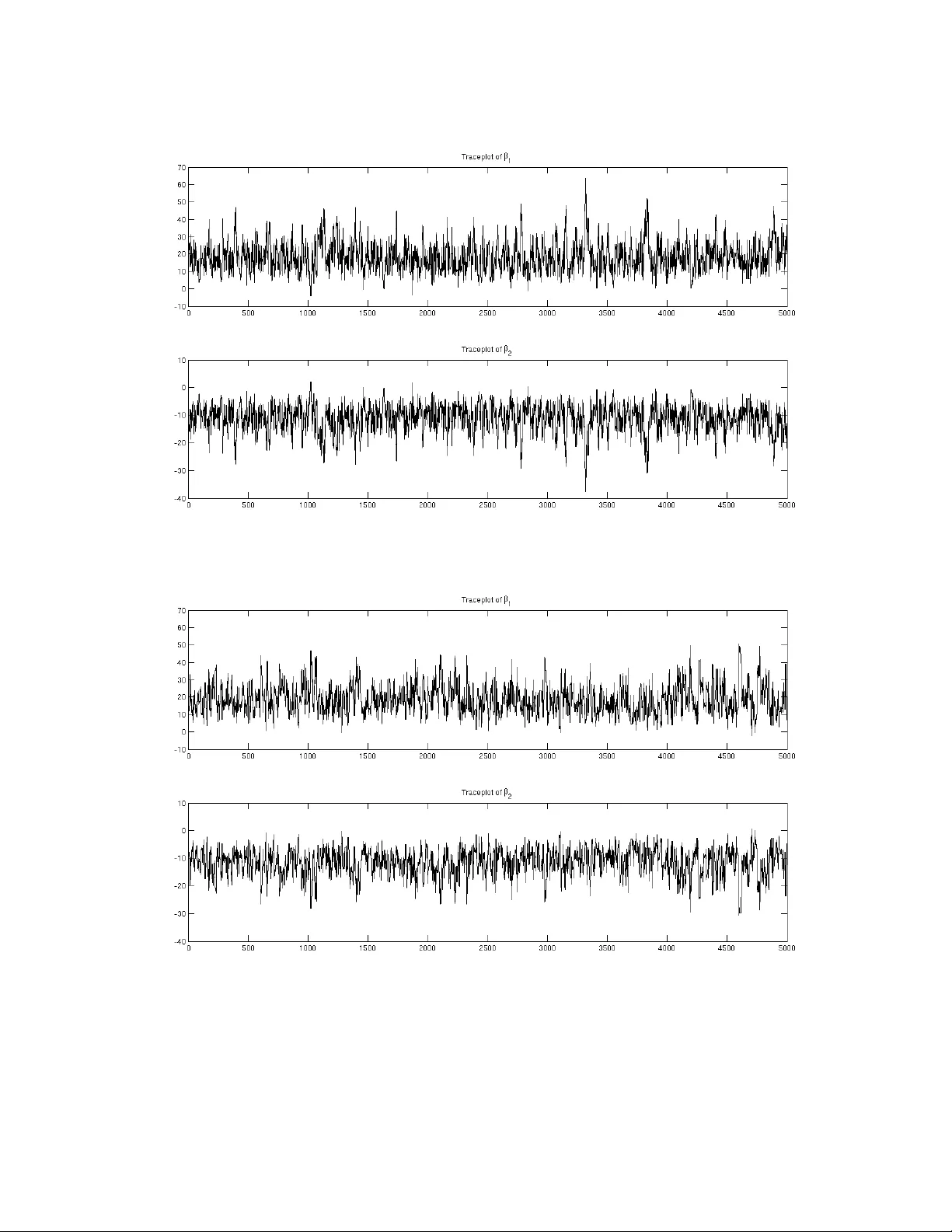
Mark ov Chain Monte Carlo Based on Deterministic T ransf ormations Somak Dutta ∗ Department of Statistics Uni v ersity of Chicago and Sourabh Bhattacharya Bayesian and Interdisciplinary Research Unit Indian Statistical Institute Abstract In this article we propose a nov el MCMC method based on deterministic transformations T : X ×D → X where X is the state-space and D is some set which may or may not be a subset of X . W e refer to our ne w methodology as Transformation-based Marko v chain Monte Carlo (TMCMC). One of the remarkable advantages of our proposal is that e ven if the underlying target distrib ution is very high-dimensional, deterministic transformation of a one-dimensional random variable is suffi- cient to generate an appropriate Mark ov chain that is guaranteed to con v er ge to the high-dimensional target distrib ution. Apart from clearly leading to massi ve computational savings, this idea of de- terministically transforming a single random v ariable v ery generally leads to excellent acceptance rates, even though all the random v ariables associated with the high-dimensional target distribution are updated in a single block. Since it is well-known that joint updating of many random variables using Metropolis-Hastings (MH) algorithm generally leads to poor acceptance rates, TMCMC, in this regard, seems to provide a significant advance. W e v alidate our proposal theoretically , establishing the con v ergence properties. Furthermore, we show that TMCMC can be very ef fecti vely adopted for simulating from doubly intractable distributions. W e sho w that TMCMC includes hybrid Monte Carlo (HMC) as a special case. W e also contrast TMCMC with the generalized Gibbs and Metropolis methods of Liu and Y u (1999), Liu and Sabatti (2000) and Kou et al. (2005), pointing out that even though the latter also use transformations, their goal is to seek improv ement of the standard Gibbs and Metropolis Hastings algorithms by adding a transformation-based step, while TMCMC is an altogether ne w and general methodology for simu- lating from intractable, particularly , high-dimensional distributions. TMCMC is compared with MH using the well-kno wn Challenger data, demonstrating the effec- ti veness of of the former in the case of highly correlated v ariables. Moreover , we apply our methodol- ogy to a challenging posterior simulation problem associated with the geostatistical model of Diggle ∗ Corresponding e-mail: sdutta@galton.uchicago.edu 1 et al. (1998), updating 160 unknown parameters jointly , using a deterministic transformation of a one-dimensional random variable. Remarkable computational savings as well as good conv ergence properties and acceptance rates are the results. K eywor ds: Geostatistics; High dimension; In verse transformation; Jacobian; Metropolis-Hastings algo- rithm; Mixture proposal 1 Intr oduction Marko v chain Monte Carlo (MCMC) has rev olutionized statistical, particularly , Bayesian computation. In the Bayesian paradigm, howe ver complicated the posterior distribution may be, it is always possible, in principle, to obtain as many (dependent) samples from the posterior as desired, to make inferences about posterior characteristics. But in spite of the obvious success story enjoyed by the theoretical side of MCMC, satisfactory practical implementation of MCMC often encounters sev ere challenges, particularly in very high-dimensional problems. These challenges may arise in the form of the requirement of enor- mous computational ef fort, often requiring in versions of v ery high-dimensional matrices, implying the requirement of enormous computation time, e ven for a single iteration. Given that such high-dimensional problems typically con ver ge extremely slowly to the target distribution triggered by complicated poste- rior dependence structures between the unkno wn parameters, astronomically large number of iterations (of the order of millions) are usually necessary . This, coupled with the computational e xpense of indi vid- ual iterations, generally mak es satisfactory implementation of MCM C, and hence, satisfactory Bayesian inference, infeasible. That this is the situation despite steady technological advancement, is some what disconcerting. 1.1 Over view of the contrib utions of this paper In an attempt to ov ercome the problems mentioned above, in this paper we propose a nov el method- ology that can jointly update all the unknown parameters without compromising the acceptance rate, unlike in Metropolis-Hastings (MH) algorithm. In fact, we show that ev en though a very large num- ber of parameters are to be updated, these can be updated by simple deterministic transformations of a single, one-dimensional random variable, the distribution of which can be chosen very flexibly . As can be already anticipated from this brief description, indeed, this yields an e xtremely fast simulation algorithm, thanks to the singleton random variable to be fle xibly simulated, and the subsequent simple 2 deterministic transformation, for example, additi ve transformation. It is also possible, maybe more ef- ficient sometimes, to generate more than one, rather than a single, random v ariables, from a flexible multi v ariate (generally independent), b ut lo w-dimensional distribution. W e refer to our new methodol- ogy as T ransformation-based MCMC (TMCMC). W e show that by generating as many random variables as the number of parameters, instead of a single/fe w random variables, TMCMC can be reduced to a MH algorithm with a specialized proposal distribution. Another popular MCMC methodology , the hybrid Monte Carlo (HMC) method, which relies upon a specialized deterministic transformation, will be sho wn to be a special case of TMCMC. W e also provide a brief overvie w of the transformation-based generalized Gibbs and Metropolis methods of Liu and Y u (1999), Liu and Sabatti (2000) and K ou et al. (2005), and point out their differ - ences with TMCMC, also arguing that TMCMC can be far more ef ficient at least in terms of computa- tional gains. Apart from illustrating TMCMC on the well-kno wn Challenger data set, and demonstrating its supe- riority over existing MH methods, we successfully apply TMCMC with the mere simulation of a single random variable, to update 160 unknown parameters in e very iteration, in the challenging geospatial problem of Diggle et al. (1998). The computational challenges in volv ed with this and similar geospa- tial problems hav e motiv ated varieties of MCMC algorithms and deterministic approximations to the posterior in the literature (see, e. g. Rue (2009), Christensen (2006) and the references therein). W ith our TMCMC algorithm we ha ve been able to perform 5 . 5 × 10 7 iterations (in a fe w days) and obtain reasonable con ver gence. W e also sho w ho w TMCMC can be adopted to significantly improve computational ef ficiency in dou- bly intractable problems, where the posterior , apart from being intractable, also in volv es the normalizing constant of the lik elihood—the crucial point being that the normalizing constant, which depends upon unkno wn parameters, is also intractable. The rest of this article is structured as follo ws. In Section 2 we introduce our new TMCMC method based on transformations. The uni v ariate and the multiv ariate cases are considered separately in Sec- tions 2.1 and 2.2 respecti vely . In Section 3 we study in details the role and ef ficiency of a singleton  in updating high-dimensional Markov chains using TMCMC. Illustration of TMCMC with singleton  using the Challenger data and comparison with a popular MCMC technique are provided in Section 4. Application of TMCMC with single  to the 160-dimensional geospatial problem of Diggle et al. (1998) 3 is detailed in Section 5. Section 6 shows ho w TMCMC may be applied to the bridge-exchange algorithm of Murray et al. (2006) in doubly intractable problems to speed-up computation. Finally , conclusions and ov ervie w of future work are pro vided in Section 7. Further in vestigations and additional details are provided in the supplement Dutta and Bhattacharya (2013), whose sections, figures and tables hav e the prefix “S-” when referred to in this paper . The con- tents of the supplement are as follo ws. Section S-1 contains the proof of detailed balance for TMCMC, Section S-2 provides the general TMCMC algorithm for a one-dimensional proposal, while Section S- 3 contains details on con ver gence properties of additiv e TMCMC. In Section S-4 we provide a more structured version of the general TMCMC algorithm of Section S-2, proving detailed balance of this algorithm in Section S-5. Detailed in vestigation of acceptance rate of additi ve TMCMC and comparison with that of random walk MH (R WMH) is carried out in Section S-6. In Sections S-7 and S-8 respec- ti vely , comparisons of TMCMC with HMC and generalized Gibbs/Metropolis methods of Liu and Y u (1999), Liu and Sabatti (2000), and K ou et al. (2005) are provided. Examples of TMCMC for discrete state spaces are provided in Section S-9. 2 MCMC algorithms based on transf ormations on the state–space In this section we propose and study the TMCMC algorithms. First, we construct it for state-spaces of dimension one. This case is not of much interest because the state space is similar to the real line and numerical integration is quite efficient in this scenario. Ne vertheless, construction of the TMCMC algorithm for one dimensional problems helps to generalize it to higher dimensions and points out its connections (similarities in one-dimension and dissimilarities in higher dimensions) with the MH algo- rithm. In Sections 2.2 and 3 the TMCMC algorithm is generalized to higher dimensional state-spaces, the latter section considering the utility of single  in high dimensions. 2.1 Univ ariate case Before pro viding the formal theory we first provide an informal discussion of our ideas with a simple example in volving the additi ve transformation. 4 2.1.1 Inf ormal discussion In order to obtain a valid algorithm based on transformations, we need to design appropriate “move types” so that detailed balance and irreducibility hold. Giv en that we are in the current state x , we can propose the “forward move” x 0 = x +  ; here  > 0 is a simulation from some arbitrary density of the form g (  ) I (0 , ∞ ) (  ) . T o move back to x from x 0 , we need to apply the “backward transformation” x 0 −  . In general, giv en  and the current state x , we shall denote the forw ard transformation by T ( x,  ) , and the backward transformation by T b ( x,  ) . The forward and the backw ard transformations need to be 1-to-1. In other words, for any fix ed  , gi ven x 0 the backward transformation must be such that x can be retrie ved uniquely . Since this must hold good for e very x in the state space, the transformation must be onto as well. Similarly , for any fixed  , there must e xist x such that the forw ard transformation leads to arbitrarily chosen x 0 in the state space uniquely , implying that this transformation is also 1-to-1 and onto. If, giv en  and x 0 , say , more than one solution exist, then return to the current value x can not be ensured, and this makes detailed balance, a requirement for stationarity of the underlying Marko v chain, hard to satisfy . The detailed balance requirement also demands that, gi ven x , the regions covered by the forward and the backward transformations are disjoint. For example, in our additi ve transformation case, the forward transformation always takes x to some unique x 0 , where x 0 > x . T o return from x 0 to x , it is imperativ e that the backward transformation decreases the value of x 0 to giv e back x . Thus, if the forward transformation always increases the current value x , the backward transformation must always decrease x . In other words, the re gions cov ered by the two transformations are disjoint. Since x is led to x 0 by the forward transformation and x 0 is taken back to x by the backward transformation, we must hav e T ( T b ( x,  ) ,  ) = x . Also, the sequence of forward and backward transformations can be changed to achie ve the same effect, that is, we must also ha ve T b ( T ( x,  ) ,  ) = x . In the abo ve discussion we indicated the use the same  for updating x to x 0 and for moving back from x 0 to x . An important adv antage associated with this strategy is that whatev er the choice of the density g (  ) I (0 , ∞ ) (  ) , it will cancel in the acceptance ratio of our TMCMC algorithm, resulting in a welcome simplification. Thanks to bijection each of the forward and the backward transformations will be equipped with their respectiv e in verses. In general, we denote by T ( x,  ) and T b ( x,  ) the forw ard and the back- ward transformations, and by T − 1 ( x,  ) and T b − 1 ( x,  ) their respectiv e in verses. Note that for fixed  , T − 1 ( x,  ) = T b ( x,  ) , and T b − 1 ( x,  ) = T ( x,  ) , but the general in verses must be defined by eliminating 5  . For instance, substituting  = x 0 − x for the forward transformation yields T ( x,  ) = T ( x, x 0 − x ) = x + ( x 0 − x ) = x 0 . Defining T − 1 ( x, x 0 ) = x 0 − x , it then follo ws that T ( x, T − 1 ( x, x 0 ))= x 0 = T − 1 ( x, T ( x, x 0 )) , sho wing that T − 1 is the in verse of T in the above sense. Similarly , T b − 1 can also be defined. 2.1.2 F ormal set-up Suppose T : X × D → X for some D (possibly a subset of X ) is a totally differentiable transformation such that 1. for ev ery fixed  / ∈ N 1 , the transform x 7− → T ( x,  ) is bijecti ve and dif ferentiable and that the in verse is also dif ferentiable. 2. for ev ery fixed x / ∈ N 2 , the transform  7− → T ( x,  ) is injectiv e. where N 1 and N 2 are π -ne gligible sets. Further suppose that the Jacobian J ( x,  ) =     ∂ ( T ( x,  ) ,  ) ∂ ( x,  )     is non-zero almost e verywhere. Suppose there is a subset Y of D such that ∀ x / ∈ N 2 the sets T ( x, Y ) and T b ( x, Y ) are disjoint, where T b ( x,  ) is the backward transformation defined by: T  T b ( x,  ) ,   = T b ( T ( x,  ) ,  ) = x Example: T ransformations on One dimensional state–space 1. (additiv e transformation) Suppose X = D = R and T ( x,  ) = x +  . Let T b ( x,  ) = x −  . This transformation is basically the random walk if  is a random quantity . Notice that if we may choose Y = (0 , ∞ ) , then T ( x, Y ) = ( x, ∞ ) , T b ( x, Y ) = ( −∞ , x ) and we can characterize the transformation as a forward move or a backward mov e according as  ∈ or / ∈ Y . Notice that here N is the empty set and for all  ∈ D the map x 7− → T ( x,  ) is a bijection. 2. (log–additiv e transformation) Suppose X = D = (0 , ∞ ) and T ( x,  ) = x . F or all x ∈ X , T b ( x,  ) = x/ ; Y = (0 , 1) . 3. (multiplicativ e transformation) Let X = R = D , T ( x,  ) = x . Then N 1 = N 2 = { 0 } , for all  6 = 0 , T b ( x,  ) = x/ ; Y = ( − 1 , 1) − { 0 } . 6 Suppose further that g is a density on Y and that 0 < p < 1 . Then the MCMC algorithm based on transformation is gi ven in Algorithm 2.1 Algorithm 2.1 MCMC algorithm based on transformation (univariate case) • Input: Initial value x 0 , and number of iterations N . • For t = 0 , . . . , N − 1 1. Generate  ∼ g ( · ) and u ∼ U (0 , 1) independently 2. If 0 < u < p , set x 0 = T ( x t ,  ) and α ( x t ,  ) = min  1 , 1 − p p π ( x 0 ) π ( x t ) J ( x,  )  3. Else if p < u < 1 set x 0 = T b ( x t ,  ) and α ( x t ,  ) = min  1 , p 1 − p π ( x 0 ) π ( x t ) 1 J ( x,  )  4. Set x t +1 =    x 0 with probability α ( x t ,  ) x t with probability 1 − α ( x t ,  ) • End for Notably , the acceptance probability is independent of the distribution g ( · ) , even if it is not symmetric. The algorithm can be sho wn to be a special case of MH algorithm with the mixture proposal density: q ( x → z ) = p g ( T − 1 ( x, z ))     ∂ T − 1 ( x, z ) ∂ z     I ( z ∈ T ( x, Y )) + (1 − p ) g ( T b − 1 ( x, z ))      ∂ T b − 1 ( x, z ) ∂ z      I ( z ∈ T b ( x, Y )) (2.1) where the in verses are defined by 1. T ( x, T − 1 ( x, z )) = z = T − 1 ( x, T ( x, z )) , ∀ z ∈ T ( x, Y ) 2. T b ( x, T b − 1 ( x, z )) = z = T b − 1 ( x, T b ( x, z )) , ∀ z ∈ T b ( x, Y ) 7 In Section S-1 we sho w that detailed balance holds for the abov e algorithm. This ensures that our TMCMC methodology has π as the stationary distrib ution. Although in this uni v ariate case TMCMC is an MH algorithm with the specialized mixture density (2.1) as the proposal mechanism, this proposal distribution becomes singular in general in higher dimensions. W e remark that TMCMC maybe particularly useful for impro ving the mixing properties of the Marko v chain. For instance, if there are distinct modes in se veral disjoint regions of state space, then standard MH algorithms tend to get trapped in some modal regions, particularly if the proposal distri- bution has small variance. Higher variance, on the other hand, may lead to poor acceptance rates in standard MH algorithms. Gibbs sampling is perhaps more prone to mixing problems due to the lack of tuning facilities. For multimodal tar get distributions, mixture proposal densities are often recommended. For instance, Guan and Krone (2007) theoretically prov e that a mixture of two proposal densities results in a “rapidly mixing” Marko v chain when the target distrib ution is multimodal. Our proposal, which we hav e shown to be a mixture density in the one-dimensional case, seems to be appropriate from this perspecti ve. Indeed, in keeping with this discussion, Dutta (2012), apart from sho wing that the multi- plicati ve transformation is geometrically er godic e ven in situations where the standard proposals fail to be so, demonstrated that it is v ery ef fectiv e for bimodal distributions. These arguments demonstrate that a real advantage of TMCMC (also of other transformation-based methods as in Liu (2001)) comes forth when the transformations associated with our method identify a subspace moving within which allo ws to explore re gions that are otherwise separated by valle ys in the probability function. Ef ficient choice of transformations of course depends upon the target distrib ution. In higher dimensions our proposal does not admit a mixture form but since the principles are similar , it is not unreasonable to expect good con vergence properties of TMCMC in the cases of high-dimensional and/or multimodal target densities. In the multidimensional case, which makes use of multi v ariate trans- formations (which we introduce next), reasonable acceptance rates can also be ensured, in spite of the high dimensionality . This we show in Section S-6, and illustrate with the Challenger data problem and particularly with the geostatistical problem. Moreov er , the multiv ariate transformation method brings out other significant adv antages of our method, for instance, computational speed and the ability to ov ercome mixing problems caused by highly correlated v ariables. 8 2.2 Multiv ariate case Suppose no w that X is a k -dimensional space of the form X = Q k i =1 X i so that T = ( T 1 , . . . , T k ) where each T i : X i × D → X i , for some set D , are transformations as in Section 2.1. Let z = ( z 1 , . . . , z k ) be a vector of indicator variables, where, for i = 1 , . . . , k , z i = 1 and z i = − 1 indicate, respecti vely , application of forward transformation and backward transformation to x i . Giv en any such indicator vector z , let us define T z = ( g 1 , g 2 , . . . , g k ) where g i =    T b i if z i = − 1 T i if z i = 1 . Corresponding to any giv en z , we also define the following ‘conjugate’ vector z c = ( z c 1 , z c 2 , . . . , z c k ) , where z c i =    1 if z i = − 1 − 1 if z i = 1 . W ith this definition of z c , T z c can be interpreted as the conjugate of T z . Since 2 k v alues of z are possible, it is clear that T , via z , induces 2 k many types of ‘moves’ of the forms { T z i ; i = 1 , . . . , 2 k } on the state–space. Suppose no w that there is a subset Y of D such that the sets T z i ( x , Y ) and T z j ( x , Y ) are disjoint for ev ery z i 6 = z j . Examples: T ransformations on higher dimensional state–space 1. (Additiv e transformation) Suppose X = D = R 2 . W ith two positiv e scale parameters a 1 and a 2 , we can then consider the following additi ve transformation: T (1 , 1) ( x ,    ) = ( x 1 + a 1  1 , x 2 + a 2  2 ) , T ( − 1 , 1) ( x ,    ) = ( x 1 − a 1  1 , x 2 + a 2  2 ) , T (1 , − 1) ( x ,    ) = ( x 1 + a 1  1 , x 2 − a 2  2 ) and T ( − 1 , − 1) ( x ,    ) = ( x 1 − a 1  1 , x 2 − a 2  2 ) . W e may choose Y = (0 , ∞ ) × (0 , ∞ ) . 2. (Multiplicativ e transformation) Suppose X = D = R × (0 , ∞ ) . Then we may consider the follo wing multiplicati ve transformation: T (1 , 1) ( x ,    ) = ( x 1  1 , x 2  2 ) , T ( − 1 , 1) ( x ,    ) = ( x 1 / 1 , x 2  2 ) , T (1 , − 1) ( x ,    ) = ( x 1  1 , x 2 / 2 ) and T ( − 1 , − 1) ( x ,    ) = ( x 1 / 1 , x 2 / 2 ) . W e may let Y = { ( − 1 , 1) − { 0 }}× (0 , 1) . 3. (Additiv e-multiplicati ve transformation) Suppose X = D = R × (0 , ∞ ) . It is possible to combine additi ve and multiplicati ve transformations in the follo wing manner: T (1 , 1) ( x ,    ) = ( x 1 +  1 , x 2  2 ) , T ( − 1 , 1) ( x ,    ) = ( x 1 −  1 , x 2  2 ) , T (1 , − 1) ( x ,    ) = ( x 1 +  1 , x 2 / 2 ) and T ( − 1 , − 1) ( x ,    ) = ( x 1 −  1 , x 2 / 2 ) . W e may let Y = (0 , ∞ ) × (0 , 1) . 9 The abov e examples can of course be generalized to arbitrary dimensions. Also, it is clear that it is possible to construct valid transformations in high-dimensional spaces using combinations of valid transformations on one-dimensional spaces. No w suppose that g is a density on Y , and, for i = 1 , . . . , 2 k , let P i = P ( T z i ) be the probability of the move-type T z i . W e assume that for each i , P i > 0 and P 2 k i =1 P i = 1 . Note that this requires us to specify the 2 k -dimensional probability vector , which seems to be a daunting task for lar ge k . Howe ver , in Section 3.1 we show that this difficulty can be overcome by considering a product form of the mov e- type probabilities induced by a mechanism of simulating z , which facilitates the choice of appropriate mov e-types from the very large set of av ailable mov e-types. This mechanism is also highly efficient computationally . The MCMC algorithm based on transformations is gi ven in Algorithm 2.2. Algorithm 2.2 MCMC algorithm based on transformation (multivariate case) • Input: Initial value x (0) , and number of iterations N . • For t = 0 , . . . , N − 1 1. Generate    ∼ g ( · ) and an index i ∼ M (1; P 1 , . . . , P 2 k ) independently. Actually, simulation from the multinomial distribution is not necessary; see Section 3.1 for an efficient and computationally inexpensive method of generating the index even when the number of move-types far exceeds 2 k . 2. x 0 = T z i ( x ( t ) ,    ) and α ( x ( t ) ,    ) = min  1 , P ( T z c i ) P ( T z i ) π ( x 0 ) π ( x ( t ) )     ∂ ( T z i ( x ( t ) ,    ) ,    ) ∂ ( x ( t ) ,    )      3. Set x ( t +1) =    x 0 with probability α ( x ( t ) ,    ) x ( t ) with probability 1 − α ( x ( t ) ,    ) • End for 10 In light of the above algorithm, it can be seen that for each of the transformations in the abov e examples, a mixture proposal of the form (2.1) is induced. It will, howe ver , be pointed out in Section 3 that a singleton  suffices for updating multiple random variables simultaneously , which would imply singularity of the underlying proposal distribution. Notice that for arbitrary dimensions the additi ve transformation reduces to the R WMH. Algorithm 2.2 indicates that updating highly correlated variables can be done naturally with TM- CMC: for instance, in Example 1 of this section one may select T (1 , 1) ( x ,    ) and T ( − 1 , − 1) ( x ,    ) with high probabilities if x 1 and x 2 are highly positi vely correlated and T ( − 1 , 1) ( x ,    ) and T (1 , − 1) ( x ,    ) may be se- lected with high probabilities if x 1 and x 2 are highly negati vely correlated. 3 V alidity and usefulness of singleton  in implementing TMCMC in high dimensions Crucially , a singleton  suffices to ensure the v alidity of our algorithm, ev en though many variables are to be updated. This indicates a very significant computational adv antage over all other MCMC-based methods: for instance, complicated simulation of hundreds of thousands of variables may be needed for any MCMC-based method, while, for the same problem, a single simulation of our methodology will do. Indeed, in Section 5 we update 160 v ariables using a single  in the geostatistical problem of Diggle et al. (1998). This singleton  also ensures that a mixture MH proposal density corresponding to our TMCMC method does not exist. The last fact sho ws that TMCMC can not be a special case of the MH algorithm. On the other hand, assuming that instead of singleton  , there is an  i associated with each of the variables x i ; i = 1 , . . . , k , then again TMCMC boils down to the MH algorithm, and, as in the univ ariate case, here also our transformations would induce a mixture proposal distrib ution for the algorithm, consisting of 2 k mixture components each corresponding to a multi v ariate transformation. Using singleton  , for transformations other than the additiv e transformation, it is necessary to in- corporate extra move types having positi ve probability which change one v ariable using forward or backward transformation, keeping the other variables fixed at their current v alues. Consider for instance, Example 3 of Section 2.2. The example indicates that, with a singleton  , it is only possible to mov e from ( x 1 , x 2 ) to either of the follo wing states: ( x 1 + , x 2  ) , ( x 1 − , x 2  ) , ( x 1 + , x 2 / ) and ( x 1 − , x 2 / ) with 11 positi ve probabilities. In addition, we could specify that the states ( x 1 , x 2  ) , ( x 1 , x 2 / ) , ( x 1 + , x 2 ) and ( x 1 − , x 2 ) also hav e positi ve probabilities to be visited from ( x 1 , x 2 ) in one step. W e will need to specify the visiting probabilities P i > 0; i = 1 , . . . , 8 such that P 8 i =1 P i = 1 . A general method of specifying the mov e-type probabilities, which also preserves computational efficienc y , is discussed in Section 3.1. Inclusion of the extra mov e types ensures irreducibility and aperiodicity (the definitions are provided in Section S-3) of the Markov chain. It is easy to see that ev en for higher dimensions irreducibility and aperiodicity can be enforced by bringing in move types of similar forms that updates one variable keep- ing the remaining variables fixed. One only needs to bear in mind that the move types must be included in pairs, that is, a move type that updates only the i -th co-ordinate x i using forward transformation and the conjug ate mo ve type that updates only x i using the backward transformation both must hav e positi ve probability of selection. W ith single  and the addition of the extra mo ve types Algorithm 2.2 requires only slight modification. As in Section 2.2 let z = ( z 1 , . . . , z k ) be the v ector of indicator v ariables, but no w , in addition to the v alues 1 and − 1 as before, z i can take the value 0 as well, indicating no change to x i . The generalized definition of z i can be expressed as follo ws: z i =          1 indicates forward transformation to x i 0 indicates no change to x i − 1 indicates negati ve transformation to x i . Gi ven any such indicator v ector z , we define as before T z = ( g 1 , g 2 , . . . , g k ) where now we e xtend the definition of g i to the follo wing: g i =          T b i if z i = − 1 x i if z i = 0 T i if z i = 1 . W e also need to extend the definition of the conjugate vector: gi ven z , we define the conjugate v ector z c = ( z c 1 , z c 2 , . . . , z c k ) , where z c i =          1 if z i = − 1 0 if z i = 0 − 1 if z i = 1 . In this definition of z i , 3 k v alues of z are possible, so that we no w ha ve 3 k possible mov e-types the forms { T z i ; i = 1 , . . . , 3 k } on the state–space. Now note that the move type induced by z = (0 , 0 , . . . , 0) does 12 not propose any change to the current state x . Hence, we discard this move, and consider the remaining 3 k − 1 move-types for our TMCMC methodology . No w suppose that g is a density on Y , and, for i = 1 , . . . , 3 k − 1 , let P i = P ( z i ) be the probability of the mo ve-type T z i . W e assume that for each i , P i > 0 and P 3 k − 1 i =1 P i = 1 . W ith these minor modifications Algorithm (2.2) goes through with    replaced by the singleton  . For the sake of completeness, we present our general TMCMC algorithm based on a single  in Section S-2 (Algorithm S-2.1). This strategy works for all transformations, including the examples in Section 2.2 where we now assume equality of all the components of    . Only additional mo ve types are in volv ed for transformations in general. Howe ver , we prove in Section S-3 that the additiv e transformation does not require the additional mo ve types. Also taking account of the inherent simplicity of this transformation, the additi ve transformation is our automatic choice for the applications reported in this paper . 3.1 Flexible and computationally efficient specification of the move-type proba- bilities An apparent drawback of Algorithms 2.2 and S-2.1 is the dif ficulty of specifying the move-type prob- abilities p ( z ) for all possible values of z . For large dimension k , manual specification of such high- dimensional probability v ector is clearly infeasible. Moreover , step 1 of Algorithms 2.2 and S-2.1 refers to simulation from a multinomial distribution in volving the v ery high-dimensional move-type probability vector . But simulation from such a high-dimensional multinomial distrib ution can be computationally burdensome in the extreme if traditional methods of multinomial simulation are used, ev en if specifi- cation of the move-type probability vector is at all possible. In this section we show how both these problems can be avoided. The key idea is to note that the move-type probabilities of T z can be induced by assigning probabilities to all possible values of z ; a simple, but useful way is to assign positiv e prob- abilities to {− 1 , 0 , 1 } , the possible v alues of each component z i of z . The latter induces a probability distribution on the set of av ailable move-types T z , and hence on the high-dimensional multinomial dis- tribution. Simulation of z by drawing z i independently for i = 1 , . . . , k yields the mo ve-type T z , thus obviating the requirement of simulation from the high-dimensional multinomial distrib ution using tradi- tional methods. In this mechanism specification of only the probabilities P r ( Z i = 1) and P r ( Z i = − 1) for i = 1 . . . , k , are required, which is manageable. Details follo w . 13 Consider a k ( ≥ 1) -dimensional target distribution, with associated random v ariables x = ( x 1 , . . . , x k ) . Then, we can implement the follo wing simple rule. Giv en x , let the forward and the backward trans- formations be applied to x i with probabilities p i and q i , respectiv ely . W ith probability 1 − p i − q i , x i remains unchanged. W e no w define z to be a random vector such that the random v ariable z i takes values − 1 , 0 , 1 , with probabilities q i , 1 − p i − q i , p i , respectiv ely . The values − 1 , 0 , 1 correspond, as before, to backward transformation, no change, and forward transformation, respecti vely . This rule, which is to be applied to each of i = 1 , . . . , k coordinates, includes all possible move types, including the one where none of the x i is updated, that is, x is taken to x . Since the mov e-type x 7→ x is redundant, this is to be rejected whenev er it appears. In other words, we would keep simulating the discrete random vector z = ( z 1 , . . . , z k ) until at least one z i 6 = 0 , and would then select the corresponding mov e type. For any dimension, this is a particularly simple and computationally ef ficient ex ercise, since the rejection region is a singleton, and has very small probability (particularly in high dimensions) if either of p i and q i is high for at least one i . Since no w we induce the probability distribution of T z through z , we denote P ( T z ) by P ( z ) . The abov e method implies that the probability of a mov e-type, giv en z , is of the form P ( z ) = C Y { i 1 : z i 1 =1 } p i 1 Y { i 2 : z i 2 = − 1 } q i 2 Y { i 3 : z i 3 =0 } (1 − p i 3 − q i 3 ) , and C is the normalizing constant, which arose due to rejection of the move type x 7→ x . This normal- izing constant cancels in the acceptance ratio, and so it is not required to calculate it explicitly , another instance of preserv ation of computational ef ficiency . Note that the probability of the conjugate mov e- type is P ( z c ) = C Y { i 1 : z c i 1 =1 } p i 1 Y { i 2 : z c i 2 = − 1 } q i 2 Y { i 3 : z c i 3 =0 } (1 − p i 3 − q i 3 ) = C Y { i 1 : z i 1 = − 1 } p i 1 Y { i 2 : z i 2 =1 } q i 2 Y { i 3 : z i 3 =0 } (1 − p i 3 − q i 3 ) , so that the factor Q { i 3 : z i 3 =0 } (1 − p i 3 − q i 3 ) cancels in the acceptance ratio, further simplifying computation. Algorithm 3.1 gi ves the simplified TMCMC algorithm based on a singleton  . Algorithm 3.1 Simplified TMCMC algorithm based on a single  . • Input: Initial value x (0) , and number of iterations N . 14 • For t = 0 , . . . , N − 1 1. Generate  ∼ g ( · ) and simulate z by generating z i ∼ M (1; p i , q i , 1 − p i − q i ) independently for i = 1 , . . . , k . 2. x 0 = T z ( x ( t ) ,  ) and α ( x ( t ) ,  ) = min  1 , P ( z c ) P ( z ) π ( x 0 ) π ( x ( t ) )     ∂ ( T z ( x ( t ) ,  ) ,  ) ∂ ( x ( t ) ,  )      , where P ( z c ) P ( z ) = Y { i 1 : z i 1 = − 1 } p i 1 q i 1 Y { i 2 : z i 2 =1 } q i 2 p i 2 . 3. Set x ( t +1) =    x 0 with probability α ( x ( t ) ,  ) x ( t ) with probability 1 − α ( x ( t ) ,  ) • End for For the additiv e transformation, the issues are further simplified. The random variable z i here takes the value − 1 and 1 with probabilities p i and q i = 1 − p i , respectiv ely . So, only p i needs to be specified. Since z i = 0 has probability zero in this setup, there is no need to perform rejection sampling to reject any mo ve-type. 3.2 Discussion on choices of p i and q i Interestingly , the ideas dev eloped in Section 3.1 provide us with a handle to control the move-type probabilities, by simply controlling p i and q i for each i . For instance, if some pilot MCMC analysis tells us that x i and x j are highly positi vely correlated, then we could set p i and p j (or q i and q j ) to be high provided the forward transformation on both x i and x j are increasing. On the other hand, if x i and x j are highly negati vely correlated, then we can set p i to be high (low) and q j to be low (high) and so on. Apart from these choices, there are theoretically moti v ated choices of p i and q i as well. Indeed, Dey and Bhattacharya (2013) prove, under suitable regularity conditions, that additiv e TMCMC is geometrically ergodic when p i = q i = 1 / 2 . Thus, at least for additiv e transformations, the choice p i = q i = 1 / 2 for i = 1 . . . , k , seems to be reasonable from a theoretical perspectiv e. In our TMCMC illustration of the Challenger data presented in Section 4 we choose p i , q i based on the posterior correlations obtained from a pilot MCMC analysis, whereas in the case of Rongelap data we set p i = q i = 1 / 2 . 15 3.2.1 Dependence structure on z The procedure outlined abov e simulates each co-ordinate z i independently , for i = 1 , . . . , k . But be- cause the same  is used for the transformation of each co-ordinate x i of x , the co-ordinate moves are dependent. Howe ver in addition, it is also possible to consider dependence between the compo- nents of z using a hierarchical structure. For example, for i = 1 , . . . , k , let w i = ( w i 1 , . . . , w ik ) ∼ N ( µ i , Σ i ); i = 1 , 2 , 3 , where the parameters ( µ i , Σ i ) ; i = 1 , 2 , 3 are assumed to be known. W e then set p i = exp ( w 1 i ) / P 3 j =1 exp ( w j i ) , q i = exp ( w 2 i ) / P 3 j =1 exp ( w j i ) , so that 1 − p i − q i = exp ( w 3 i ) / P 3 j =1 exp ( w j i ) . These k -variate normal distributions induce dependence between p = ( p 1 , . . . , p k ) and p = ( q 1 , . . . , q k ) . Thus, ev en though conditionally on { ( p i , q i ); i = 1 , . . . , k } z i are independent, marginalized ov er p and q , the components of z are dependent. T o achiev e the ef fect of this dependent structure in TMCMC in a theoretically valid manner , at each iteration of the TMCMC algorithm we can simulate w 1 , w 2 , w 3 from their respectiv e k -variate normal distributions, and from the simulated values obtain, for i = 1 , . . . , k , p i = exp ( w 1 i ) / P 3 j =1 exp ( w j i ) , and q i = exp ( w 2 i ) / P 3 j =1 exp ( w j i ) . T o av oid getting p i and q i too close to zero in some simulations, we can appropriately truncate the k -v ariate normal distributions. Once { ( p i , q i ); i = 1 , . . . , k } are obtained, conditionally on these probabilities, z i ; i = 1 , . . . , k will be simulated independently . Thus, the algorithm for dependent z admits the same form as Algorithm 3.1; only in the first step, simulation of p and q from their respectiv e dependent distributions must precede independent simulation of z i ; i = 1 , . . . , k . The algorithm (Algorithm S-4.1) and proof of detailed balance are provided in Sections S-4 and S-5, respecti vely . Note that for the additi ve transformation, since q i = 1 − p i , only the joint distribution of p needs to be considered, with p i = exp ( w 1 i ) / P 2 j =1 exp ( w j i ) , and it is not necessary to simulate w 3 at all. Theoretically appropriate choices of ( µ i , Σ i ) ; i = 1 , 2 , 3 will be our topic of future research but from a practical point of view , one can tune these parameters to achiev e good mixing properties and acceptance rates. 3.3 Advantages of TMCMC updating with single  Standard methods like sequential R WMH may tend to be computationally infeasible in high dimensions while inducing mixing problems due to posterior dependence between the parameters, whereas TMCMC remains free from the aforementioned problems thanks to singleton  and joint updating of all the pa- rameters. Specialized proposals for joint updating may be constructed for specific problems only; for 16 instance, block updating proposals for Gaussian Markov random fields are av ailable (Rue (2001)). But generally , efficient block updating proposals are not av ailable. Moreover , ev en in the specific problems, simulation from the specialized block proposals and calculating the resulting acceptance ratio are gen- erally computationally very expensi ve. In contrast, TMCMC with singleton  seems to be much more general and efficient. Moreov er , we demonstrate in Section 4 in connection with the Challenger data problem that TMCMC can outperform well-established block proposal mechanisms, usually based on the asymptotic co v ariance matrix of the maximum likelihood estimator (MLE), in terms of acceptance rate. 4 A pplication of TMCMC to the Challenger dataset In 1986, the space shuttle Challenger exploded during take off, killing the seven astronauts aboard. The explosion was the result of an O-ring failure, a splitting of a ring of rubber that seals the parts of the ship together . The accident w as belie ved to be caused by the unusually cold weather ( 31 0 F or 0 0 C) at the time of launch, as there is reason to believ e that the O-ring failure probabilities increase as temperature decreases. The data are provided in T able S-1 for ready reference. W e shall analyze the data with the help of well–known logit model. Our main aim is not analyzing and drawing inference since it is done already in Dalal et al. (1989), Martz and Zimmer (1992) and Robert and Casella (2004) . W e shall rather compare the dif ferent MCMC methodologies used in Bayesian inference for logit–model. Let η i = β 1 + β 2 x i where x i = t i / max t i , t i ’ s being the temperature at flight time (degrees F), i = 1 , . . . , n . and n = 23 . Also suppose y i is the indicator variable denoting failure of 0-ring. W e suppose y i ’ s independently follo w Bernoulli( π ( x i ) ). In the logit model we suppose that the log-odd ratio is a linear function of temperature at flight time, i.e., log π 1 − π = η = β 1 + β 2 x which gi ves π i = exp( η i )  (1 + exp( η i )) . In the absence of information regarding ( β 1 , β 2 ) , we specify a uniform (improper) prior for ( β 1 , β 2 ) . 17 variable method acceptance rate (%) mean std 2.5%* 25%* 50%* 75%* 97.5%* R WMH 42.17 19.119 8.078 4.909 13.481 18.475 24.227 38.176 β 1 MH 42.60 18.930 8.513 5.011 12.823 17.981 23.957 38.206 TMCMC 73.23 18.973 7.944 4.970 12.881 16.210 21.685 37.877 R WMH 48.14 -23.724 9.613 -46.272 -29.786 -22.984 -17.019 -6.7792 β 2 MH 42.60** -23.491 10.128 -46.461 -29.464 -22.353 -16.261 -6.956 TMCMC 73.23** -23.165 9.762 -46.404 -28.891 -22.282 -16.446 -7.026 T able 4.1: Summary of the posterior samples based on MCMC runs of length 100,000 out of which first 20,000 samples are discarded as burn-in. R WMH = Random walk Metropolis-Hastings, MH = Metropolis-Hastings with biv ariate normal proposal, TM- CMC = MCMC based on transformation * : posterior sample quantiles. **: same as acceptance ratio for β 1 since updated jointly . W e construct an appropriate additiv e transformation T : R 2 × R → R 2 as follo ws. First, we con- sider the form T (1 , 1) (( β 1 , β 2 ) ,  ) = ( β 1 , β 2 ) 0 + ( s 1 , s 2  ) 0 , where s 1 and s 2 are the standard errors of the maximum likelihood estimator of ( β 1 , β 2 ) 0 . Thus, we finally obtain the transformation T (1 , 1) (( β 1 , β 2 ) ,  ) = ( β 1 + 7 . 3773 , β 2 + 4 . 3227  ) and use Algorithm 3.1 with Y = (0 , ∞ ) and g (  ) ∝ exp( −  2 / 2) ,  > 0 that is, the N (0 , 1) distribution truncated to the left at zero. From the cov ariance matrix C we observe that the correlation of ˆ β 1 and ˆ β 2 is approximately − 0 . 99 and hence from our discussion in Section 3.2, setting high probabilities to the mov es T (1 , − 1) ( x ,  ) and T ( − 1 , 1) ( x ,  ) should facilitate good mixing. Follo wing the discussion in Section 3.2 we set P ((1 , 1)) = P (( − 1 , − 1)) = 0 . 01 and P ((1 , − 1)) = P (( − 1 , 1)) = 0 . 49 . Also for comparison we use the R WMH algorithm (both joint and sequential updation) and also the MH algorithm with proposal q ( β β β 0 | β β β ) = N ( β β β , Σ ) where Σ = h 2 C (we take h = 1 for our purpose) with C being the large sample cov ariance matrix of the MLE b β β β of β β β . T able 4.1 gi ves the posterior summaries and Figure 4.1 giv es the trace plots of β 1 and β 2 for TMCMC sampler and the MH sampler . It is seen that the mixing is excellent e ven though a single  has been used. Notice the excellent result of the MCMC based on transformations. The acceptance ratio is almost twice as large as those for other two MH algorithms. As remarked in Section 3.3, indeed TMCMC 18 (a) (b) Figure 4.1: T race plots of β 1 and β 2 (a) TMCMC (b) MH 19 outperformed the MH block proposal based on the lar ge sample cov ariance matrix of the MLE of β β β in terms of acceptance rate. Also for implementing TMCMC we need to simulate only one  in each step. In the R WMH with sequential updating and in MH based on biv ariate normal proposal we need tw o such  ’ s. In the R WMH we need to calculate the likelihood twice in each iteration. So, TMCMC dominates the other two in this respect. It can be easily anticipated, in light of the theoretical arguments regarding acceptance rate presented in Section S-6, that for joint R WMH the acceptance rate w ould be e ven lo wer . In Section 5, where we consider a 160-dimensional problem, we show that, that TMCMC outperforms joint R WMH by a substantially large margin in terms of acceptance rate. 5 A pplication of TMCMC to the geostatistical pr oblem of radionu- clide concentrations on Rongelap Island 5.1 Model and prior description W e no w consider the much analyzed radionuclide count data on Rongelap Island (see, for example, Diggle et al. (1997), Diggle et al. (1998), Christensen (2004), Christensen (2006)), and illustrate the performance of TMCMC with a singleton  . For i = 1 , . . . , 157 , Diggle et al. (1998) model the count data as Y i ∼ P oisson ( M i ) , where M i = t i exp { β + S ( x i ) } ; t i is the duration of observation at location x i , β is an unknown parameter and S ( · ) is a zero-mean Gaussian process with isotropic cov ariance function of the form C ov ( S ( x ? 1 ) , S ( x ? 2 )) = σ 2 exp {− ( α k x ? 1 − x ? 2 k ) δ } for any two locations x ? 1 , x ? 2 . In the above, k · k denotes the Euclidean distance between two locations, and ( σ 2 , α, δ ) are unkno wn parameters. T ypically in the literature δ is set equal to 1 (see, e. g. Christensen (2006)), which we adopt. W e assume uniform priors on the entire parameter space corresponding to ( β , log( σ 2 ) , log( α )) . 20 W e remark that since the Gaussian process S ( · ) does not define a Markov random field, the block updating proposal dev eloped by Rue (2001) is not directly applicable here. Rue (2009) attempt to de- velop deterministic approximations to latent Gaussian models, b ut the scope of such approximations is considerably restricted by the conditional independence (Gaussian Marko v random field) assumption (Banerjee (2009)). Thanks to the generality and ef ficiency of our proposed methodology , it seems most appropriate to fit the Rongelap island model using TMCMC with singleton  . 5.2 Results of additiv e TMCMC with singleton  Drawing  ∼ N (0 , 1) I (  > 0) , we considered the following additi ve transformation T ( β ,  ) = β ± 2 , T (log( σ 2 ) ,  ) = log( σ 2 ) ± 5 , T (log( α ) ,  ) = log( α ) ± 5 , T ( S ( x i ) ,  ) = S ( x i ) ± 2  ; for i = 1 , . . . , 157 The scaling factors associated with  in each of the transformations are chosen on a trial-and-error basis after experimenting with sev eral initial (pilot) runs of TMCMC. W e assigned equal probabilities to all the 2 160 mov e types. Mo ve types are selected by independently generating z i taking the v alues +1 and − 1 with equal probabilities, that is, we set p i = q i = 1 / 2 for i = 1 , . . . , 160 . As mentioned in Section 3.2 this choice of equal probabilities of forward and backward transformation is motiv ated by our result on geometric ergodicity . After discarding the first 2 × 10 7 iterations as b urn-in, we stored 1 in e very 100 iterations in the ne xt 3 . 5 × 10 7 iterations. This entire simulation took about a week to run on an ordinary laptop machine and about 3 days on a workstation. The autocorrelation functions of the variables (after further thinning by 10) of our TMCMC run, displayed in Figure 5.1, indicates reasonable mixing properties. The acceptance rate, after discarding the burn-in period, is 0.43% (considering the complete run of TMCMC after burn- in, that is, including thinning as well). 5.3 Comparison with joint R WMH W e also implemented a joint R WMH using the same additi ve transformation as in Section 5.2 but with dif ferent  ’ s for each unkno wn. Now the acceptance rate reduced to 0.0005%. These observ ations are 21 Figure 5.1: Autocorrelation plots of the variables, α , β , log σ 2 (left-panel) and s 1 , . . . , s 157 (right-panel) in the TMCMC run. broadly in keeping with the theoretical discussions presented in Section S-6. 6 A pplication of TMCMC to doubly–intractable problem Doubly–intractable distrib utions arise quite frequently in fields like circular statistics, directed graphical models, Markov point processes etc. Even some standard distributions like gamma and beta inv olve intractable normalizing constants. Formally , a density h ( y | θ ) of the data set y = ( y 1 , . . . , y n ) 0 is said to be doubly–intractable if it is of the form h ( y | θ ) = f ( y | θ ) / Z ( θ ) where Z ( θ ) is a function that is not av ailable in closed form. So if we put a prior π ( θ ) on θ , then the posterior is gi ven by π ( θ | y ) = 1 c ( y ) f ( y | θ ) Z ( θ ) π ( θ ) where c ( y ) = Z Θ f ( y | θ ) Z ( θ ) π ( θ ) dθ Thus, if we try to apply MH like algorithms then the acceptance ratio will in volv e ratio of the function Z ( · ) at two parameter points θ and θ 0 . Hence directly applying MH may not be feasible. W orks by Møller et al. (2004) and Murray et al. (2006) are significant in this field. A double MH sampler approach is taken in Liang (2010). In this section we briefly discuss the bridge–exchange algorithm by Murray et al. (2006) and sho w how our application of TMCMC in the bridge–e xchange algorithm may facilitate fast computation. Suppose M ∈ N is the bridg e size , β m = m/ ( M + 1) , m = 0 , . . . , M . Define the density p m ( x | θ , θ 0 ) ∝ f ( x | θ ) β m f ( x | θ 0 ) 1 − β m ≡ f m ( x | θ , θ 0 ) , m = 0 , . . . , M . 22 Obviously , x is of the same dimensionality as y ; that is, x = ( x 1 , . . . , x n ) 0 . Further suppose that for each m , T m ( x → x 0 | θ , θ 0 ) is a k ernel satisfying the detailed balance condition T m ( x → x 0 | θ , θ 0 ) p m ( x | θ , θ 0 ) = T m ( x 0 → x | θ , θ 0 ) p m ( x 0 | θ , θ 0 ) . No w with a proposal density q ( θ → θ 0 | y ) for the parameter , the bridge–exchange algorithm is gi ven belo w . Algorithm 6.1 The bridge–exc hange algorithm • Input: initial state θ 0 , length of the chain N , #bridge levels M . • For t = 0 , . . . , N − 1 1. Propose θ 0 ∼ q ( θ 0 ← θ t | y ) 2. Generate an auxiliary variable with exact sampling: x 0 ∼ p 0 ( x 0 | θ , θ 0 ) ≡ f ( x 0 | θ 0 ) / Z ( θ ) 3. Generate M further auxiliary variables with transition operators: x 1 ∼ T 1 ( x 0 → x 1 | θ , θ 0 ) x 2 ∼ T 2 ( x 1 → x 2 | θ , θ 0 ) . . . x M ∼ T M ( x M − 1 → x M | θ , θ 0 ) 4. Compute α ( θ 0 ← θ t ) = q ( θ 0 → θ | y ) π ( θ 0 ) f ( y | θ 0 ) q ( θ → θ 0 | y ) π ( θ ) f ( y | θ ) M Y m =0 f m +1 ( x m | θ , θ 0 ) f m ( x m | θ , θ 0 ) 5. Set θ t +1 =    θ 0 with probability α ( θ 0 ← θ t ) θ t with probability 1 − α ( θ 0 ← t t ) 23 • end for No w we see that, since each of the auxiliary variables x m , m = 1 , . . . , M , is n -dimensional, gen- eration of these auxiliary variables may be computationally demanding if the sample size n is moderate or large especially when one has to simulate from the sample space using accept-reject algorithms as in the case of circular variables. For any kernel T m which is not based on TMCMC, O ( nM ) v ariables are required to be generated from the state–space per iteration. Appealing to TMCMC, recall that with the additi ve transformation with a single  , the k ernel still satisfies the detailed balance condition. W e assume that X is a group under some binary operation and that there is a homomorphism from ( R p , +) to X for some p ∈ N . So we denote the binary operation on X by ‘ + ’ itself. Let g be a density on X . W e construct the kernels T m as follo ws: Algorithm 6.2 Construction of T m 1. Generate  ∼ g (  ) and z ∼ P ( z ) , where P ( z ) is some suitable distribution of z ; P ( z ) can be chosen as in the different versions of our TMCMC algorithm. 2. Define the vector x 0 by x 0 i =      x m − 1 ,i + a i  if z i = 1 x m − 1 ,i − a i  if z i = − 1 3. Set α ( x m − 1 → x 0 ) = min  P ( z c ) f m ( x 0 | θ , θ 0 ) P ( z ) f m ( x | θ , θ 0 ) , 1  4. Set x m =      x 0 with probability α ( x m − 1 → x 0 ) x m − 1 with probability 1 − α ( x m − 1 → x 0 ) In this way we need only O ( M ) simulations per iteration. Homomorphism from ( R p , +) to X holds in many cases, for example, in circular models where the state–space is ( − π , π ] is a group with respect to addition modulo π . 24 Figure 6.1: Left panel: Trace plot of last 1,000 samples. Right panel: exact posterior density of ν (solid line) and it’ s estimate (dash-dotted line). 6.1 Simulation study to illustrate TMCMC in bridge-exchange algorithm Here we illustrate our method for a circular model of the form h ( y | ν ) = 1 Z ( ν ) exp(cos( y + ν sin( y ))) , − π < y , ν ≤ π , W e generate a sample of size 20 from h ( y | ν = 0) and estimate the parameter ν based on this sample. The prior chosen on ν is the uniform distribution on ( − π , π ] and g ( · ) is chosen to be the normal distribution with mean 0 and v ariance 1 restricted on the set (0 , π ] . Since the components of x 0 are iid , we used P r ( Z i = 1) = P r ( Z i = − 1) = 1 / 2 and a i = 1 for each i . W e set M = 100 and chose q ( ν 0 | ν ) to be the V on-mises distrib ution with mean ν and concentration 0.5 to keep the acceptance le vel around 63%. The right panel of Figure 6.1 sho ws that the estimated posterior density of ν is v ery close to the exact posterior density . The little discrepanc y at the tails are due to the fact that ν is a circular variable and hence its support is ( − π, π ] and the density is not zero at the end points – a fact that is not incorporated in the kernel density estimator . The left panel of the same figure sho ws that the mixing is excellent. Notice that here we hav e saved 100( nM − M ) /nM = 95% simulations. 25 7 Summary , conclusions and futur e work In this paper we hav e proposed a novel MCMC method that uses deterministic transformations and move types to update the Marko v chain. W e hav e shown that our algorithm TMCMC generalizes the MH al- gorithm boiling down to MH with a specialized proposal density in one-dimensional cases. For higher dimensions if each component x i of the random v ector to be updated is associated with a distinct  i , then TMCMC again boils down to the MH algorithm with a specialized proposal density . But in dimensions greater than one, with less number of distinct  i than the size of the random vector to be updated, TM- CMC does not admit any MH representation. Se veral versions of TMCMC ha ve been detailed in this paper and in the supplement. In Section S-6 of the supplement, under reasonable regularity conditions we ha ve pro vided and compared the asymptotic forms of the acceptance rates of R WMH and additi ve TMCMC when the dimensionality increases to infinity and hav e sho wn that the latter con ver ges to zero at a much slo wer rate. That HMC is also a special case of TMCMC, is also explained in Section S-7; in addition, we ha ve pro vided asymptotic forms of the acceptance rate of HMC under reasonable re g- ularity conditions and ha ve sho wn that, as the dimensionality grows to infinity , the forms con ver ge to zero at much faster rates than additiv e TMCMC. In Section S-8 we also contrasted TMCMC with the transformation-based methods of Liu and Y u (1999), Liu and Sabatti (2000), and Kou et al. (2005). The advantages of TMCMC are more prominent in high dimensions, where simulating a single ran- dom v ariable can update many parameters at the same time, thus saving a lot of computing resources. That many v ariables can be updated in a single block without compromising much on the acceptance rate, seems to be another quite substantial adv antage provided by our algorithm. W e illustrated with examples that TMCMC can outperform MH significantly , particularly in high dimensions. The compu- tational gain of using TMCMC for simulations from doubly intractable distrib utions, is also significant, and is illustrated with an example. In this article we ha ve dev eloped TMCMC for continuous state spaces. Howe ver , in Section S-9 we show how TMCMC can be generalized to discrete state spaces as well. A complete dev elopment of TMCMC for discrete cases will be a subject of our future work. 26 Acknowledgment W e sincerely thank the revie wer whose comments hav e led to an improv ed version of our manuscript. Con versations with Dr . Ranjan Maitra has also led to improv ed presentation of some of the ideas. Refer ences S. Banerjee. Discussion: Approximate Bayesian Inference for Latent Gaussian Models by using Inte- grated Nested Laplace Approximations. J ournal of the Royal Statistical Society . Series B , 71:365, 2009. O. F . Christensen. Monte Carlo Maximum Likelihood in Model-Based Geostatistics. Journal of Com- putational and Graphical Statistics , 13:702–718, 2004. O. F . Christensen. Robust Marko v Chain Monte Carlo Methods for Spatial Generalized Linear Mixed Models. Journal of Computational and Gr aphical Statistics , 15:1–17, 2006. S. R. Dalal, E. B. Fowlk es, and B. Hoadley . Risk Analysis of the Space Shuttle: pre-Challenger Predic- tion of Failure. Journal of the American Statistical Association , 84:945–957, 1989. K. K. De y and S. Bhattacharya. On Geometric Er godicity of Additi ve Transformation Based Markov Chain Monte Carlo. T echnical report, Indian Statistical Institute, 2013. P . J. Diggle, J. A. T a wn, and R. A. Moyeed. Geostatistical Analysis of Residual Contamination from Nuclear Weapons Testing. In V . Barnet and K. F . T urkman, editors, Statistics for En vir onment 3: P ollution Assessment and Contr ol , pages 89–107. Chichester: W iley , 1997. P . J. Diggle, J. A. T awn, and R. A. Moyeed. Model-Based Geostatistics (with discussion). Applied Statistics , 47:299–350, 1998. S. Dutta. Multiplicative Random Walk Metropolis-Hastings on the Real Line. Sankhya B , 74:315–342, 2012. S. Dutta and S. Bhattacharya. Supplement to “Markov Chain Monte Carlo Based on Deterministic Transformations”, 2013. Submitted. 27 Y . Guan and S. M. Krone. Small-World MCMC and Con vergence to Multi-Modal Distributions: From Slo w Mixing to Fast Mixing. The Annals of Applied Pr obability , 17:284–304, 2007. S. C. K ou, X. S. Xie, and J. S. Liu. Bayesian Analysis of Single-Molecule Experimental Data. Applied Statistics , 54:469–506, 2005. F . Liang. A Double Metropolis-Hastings Sampler for Spatial Models with Intractable Normalizing Con- stants. Journal of Statistical Computation and Simulation , 80:1007–1022, 2010. J. Liu. Monte Carlo Strate gies in Scientific Computing . Springer-V erlag, New Y ork, 2001. J. S. Liu and S. Sabatti. Generalized Gibbs Sampler and Multigrid Monte Carlo for Bayesian Computa- tion. Biometrika , 87:353–369, 2000. J. S. Liu and Y . N. Y u. Parameter Expansion for Data Augmentation. Journal of the American Statistical Association , 94:1264–1274, 1999. H. F . Martz and W . J. Zimmer . The Risk of Catastrophic Failure of the Solid Rocket Boosters on the Space Shuttle. The American Statistician , 46:42–47, 1992. J. Møller , A. N. Pettitt, K. K. Berthelsen, and R. W . Ree ves. An Ef ficient Mark ov Chain Monte Carlo Method for Distributions with Intractable Normalising Constants. T echnical report, Department of Mathematical Sciences, Aalborg Uni versity , 2004. I. Murray , Z. Ghahramani, and D. J. C MacKay . MCMC for Doubly-Intractable Distrib utions. In R. Dechter and T . S. RIchardson, editors, Pr oceedings of the 22nd Annual Confer ence on Uncertainty in Artificial Intelligence (U AI-06) , pages 359–366. A UAI Press, 2006. C. P . Robert and G. Casella. Monte Carlo Statistical Methods . Springer-V erlag, New Y ork, 2004. H. Rue. Fast sampling of Gaussian Markov random fields. Journal of the Royal Statistical Society . Series B , 63:325–338, 2001. H. Rue. Approximate Bayesian Inference for Latent Gaussian Models by Using Inte grated Nested Laplace Approximations. Journal of the Royal Statistical Society . Series B , 71:319–392, 2009. 28