Spatio-temporal wavelet regularization for parallel MRI reconstruction: application to functional MRI

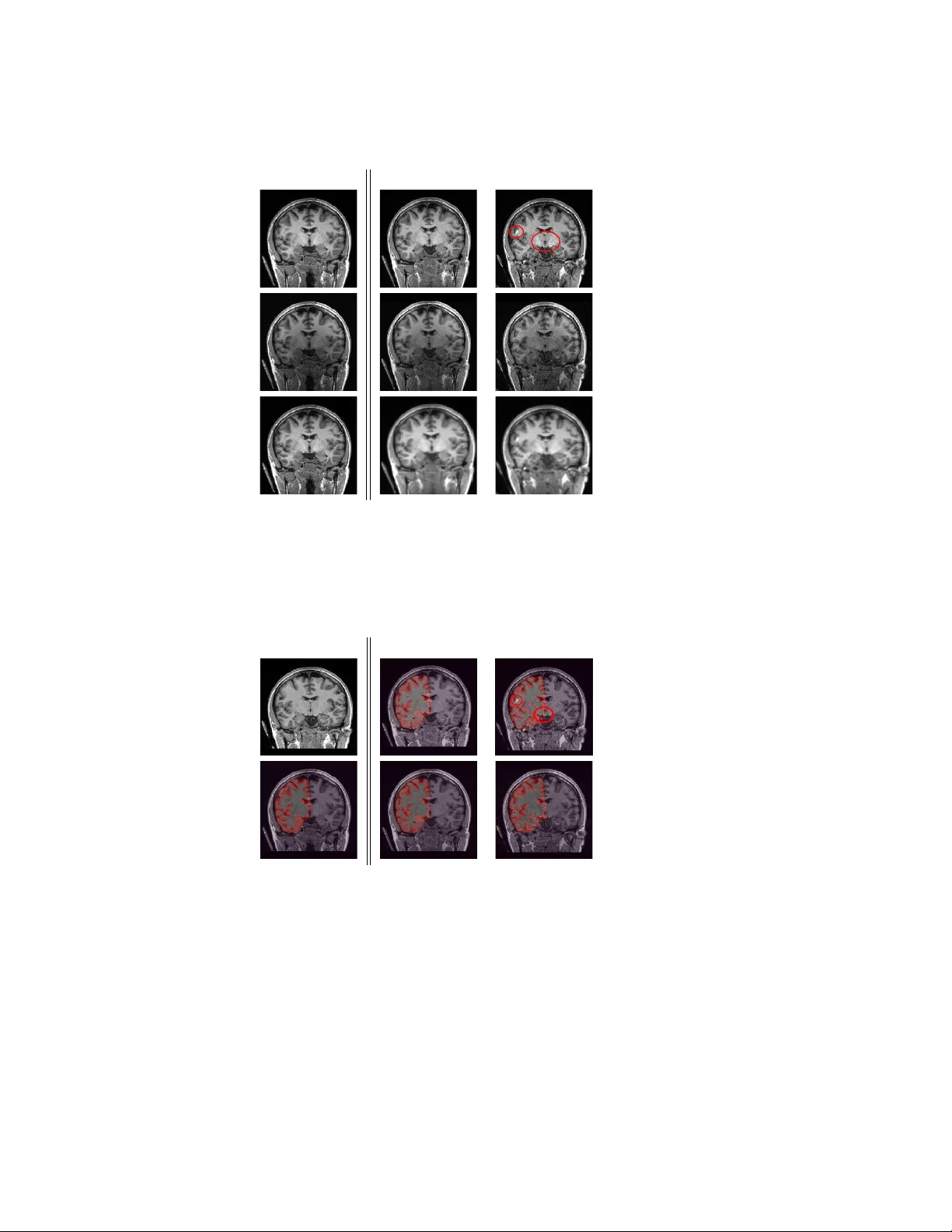
Spatio-temp o ral w avelet regula rization fo r pa rallel MRI re- construction: application to functional MRI Lotﬁ CHAARI ∗ 1 , S ´ ebastien M ´ ERIA UX 2 , Jean-Christophe PESQUET 3 and Philipp e CIUCIU 2 1 Universit y of T oulouse, IRIT - INP-ENSEEIHT, F rance. 2 LNA O, CEA-NeuroSpin, F rance. 3 LIGM, Universit y P a ris-Est, F rance. Email: lotﬁ.chaari@enseeiht.fr; sebastien.meriaux@cea.fr; jean-christophe.pesquet@univ-paris-est.fr; philippe.ciuciu@cea.fr; ∗ Co rresp onding autho r Abstract P arallel MRI is a fast imaging technique that helps in acquiring highly resolved images in space o r/and in time. The p erfo rmance of pa rallel imaging strongly dep ends on the reconstruction algo rithm, w hich can p ro ceed either in the o riginal k -space (GRAPP A, SMASH) o r in the image domain (SENSE-lik e metho ds). T o imp rove the p erformance of the widely used SENSE algorithm, 2D- or slice-sp eciﬁc regularization in the wavelet domain has been investigated. In this paper, we extend this approach using 3D-wavelet representations in o rder to handle all slices together and address reconstruction a rtifacts which propagate across adjacent slices. The gain induced b y such extension (3D-Unconstrained W avelet Regula rized -SENSE: 3D-UWR-SENSE) is validated on anatomical image reconstruction where no temp oral acquisition is considered. Another imp ortant extension accounts for temp o ral correlations that exist b etw een successive scans in functional MRI (fMRI). In addition to the case of 2D+ t acquisition schemes addressed by some other metho ds like kt -F OCUSS, our approach allo ws to deal with 3D+ t acquisition schemes which are widely used in neuroimaging. The resulting 3D-UWR-SENSE and 4D-UWR- SENSE reconstruction schemes a re fully unsup ervised in the sense that all regula rization pa rameters are estimated in the maximum lik eliho o d sense on a reference scan. The gain induced by such extensions is illustrated on b oth anatomical and functional image reconstruction, and also measured in terms of statistical sensitivity fo r the 4D- UWR-SENSE approach during a fast event-related fMRI protocol. Our 4D-UWR-SENSE algorithm outp erforms the SENSE reconstruction at the subject and group levels (15 subjects) for diﬀerent contrasts of interest (e.g., moto r or computation tasks) and using diﬀerent parallel acceleration factors ( R = 2 and R = 4 ) on 2 × 2 × 3 mm 3 EPI images. 1 Intro duction Reducing scanning time in Magnetic Resonance Imaging (MRI) exams remains a worldwide chal- lenging issue since it has to b e achiev ed while maintaining high image quality [1, 2]. The exp ected b eneﬁts are i.) to limit patient’s exp osure to the MRI environmen t either for safety or discom- fort reasons, ii.) to improv e acquisition robustness against sub ject’s motion artifacts and iii.) to 1 limit geometric distortions. One basic idea to make MRI acquisitions faster (or to impro ve spatial resolution in a ﬁxed scanning time) consists of reducing the amoun t of acquired samples in the k -space (spatial F ourier domain) and dev eloping dedicated reconstruction pip elines. T o achiev e this goal, three main research a v enues hav e b een developed so far: • p ar al lel imaging or parallel MRI that relies on a geometrical principle inv olving m ultiple receiv er coils with complementary sensitivity proﬁles. This enables the k -space undersampling along the phase enco ding direction without degrading spatial resolution or truncating the Field-Of-View (FO V). pMRI requires the unfolding of reduced FO V coil-sp eciﬁc images to reconstruct the full FO V image [3–5]. • Compr esse d Sensing (CS) MRI that exploits three ingredients: sp arsity of MR images in w av elet bases, the inc oher enc e b etw een F ourier and inv erse w av elet bases which allo ws to randomly undersample k -space and the nonline ar r e c overy of MR images by solving a conv ex but nonsmo oth ` 1 minimization problem [6, 7]. This approac h remains usable with clas sical receiv er coil but can also b e combined with parallel MRI [8, 9]. • In the dynamic MRI con text, fast parallel acquisition schemes ha v e b een prop osed to increase the acquisition rate by reducing the amount of acquired k -space samples in each frame using in terleav ed partial k -space sampling b et ween successiv e frames (UNFOLD approac h [10]). T o further reduce the scanning time, a strategy named k t -BLAST taking adv antage of b oth the spatial (actually in the k -space) and temp oral correlations b et ween successive scans in the dataset has b een pushed forward [11]. In parallel MRI (pMRI), many reconstruction metho ds lik e SMASH (Sim ultaneous Acquisi- tion of Spatial Harmonics) [3], GRAPP A (Generalized Auto calibrating Partially Parallel Acquisi- tions) [5] and SENSE (Sensitivity Enco ding) [4] hav e b een prop osed in the literature to reconstruct a full FO V image from multiple k -space undersampled images acquired on separate channels. The main diﬀerence b etw een them lies in the space on which they op erate. GRAPP A p erforms multi- c hannel full FO V reconstruction in the k -space domain whereas SENSE carries out the unfolding pro cess in the image domain: all undersampled images are ﬁrst reconstructed by inv erse F ourier transform before com bining them to un wrap the full F OV image. Also, GRAPP A is auto calibrated, whereas SENSE needs a separate coil sensitivity estimation step based on a reference scan. Note ho wev er that autocalibrated v ersions of SENSE are no w a v ailable such that the mSENSE algorithm on Siemens scanners. In the dynamic MRI context, combined strategies mixing parallel imaging and accelerated sampling schemes along the temp oral axis ha ve als o b een inv estigated. The corresp onding recon- struction algorithms hav e b een referenced to as kt -SENSE [11, 12], kt -GRAPP A [13]. Compared to mSENSE where the centre of the k -space is acquired only once at the b eginning, these metho ds hav e to acquire the central k -space area at each rep etition time, which decreases the acceleration factor. More recen tly , optimized v ersions of kt -BLAST and kt -SENSE reconstruction algorithms referenced to as kt -F OCUSS [14, 15] hav e been designed to combine the CS theory in space with F ourier or alternativ e transforms along the time axis. They enable to further reduce data acquisition time without signiﬁcan tly compromising image qualit y , pro vided that the image sequence exhibits a high degree of spatio-temporal correlation, either by nature or b y design. T ypical examples that en ter in this context are i.) dynamic MRI capturing an organ (liver, kidney , heart) during a quasi-p erio dic 2 motion due to the respiratory cycle and cardiac b eat and ii.) functional MRI based on p erio dic blo c k ed design. Ho wev er, this in terleav ed partial k -space sampling cannot b e exploited in ap erio dic dy- namic acquisition sc hemes lik e in resting state fMRI (rs-fMRI) or during fast-ev ent related fMRI paradigms [16, 17]. In rs-fMRI, sp ontaneous brain activit y is recorded without any exp erimen tal design in order to prob e intrinsic functional connectivit y [16, 18, 19]. In fast even t-related designs, the presence of jittering combined with random delivery of stimuli introduces a trial-v arying delay b et w een the stim ulus and acquisition time p oints [20]. This preven ts the use of an interlea ved k -space sampling strategy betw een successiv e scans since there is no guarantee that the BOLD resp onse is quasi-p erio dic. Because the v ast ma jority of fMRI studies in neurosciences mak e use either of rs-fMRI or fast even t-related designs [20, 21], the most reliable acquisition strategy in such con texts remains the “scan and rep eat” approach, although it is sub optimal. T o our knowledge, only one kt-c ontribution ( k t -GRAPP A [13]) has claimed its ability to accurately reconstruct fMRI images in ap erio dic paradigms. Overview of our contribution The presen t pap er therefore aims at prop osing a new 3D/(3D+t)-dimensional pMRI reconstruction algorithm that can be adopted irrespec tiv e of the nature of the enco ding scheme or the fMRI paradigm. In particular, we show that our approach outp erforms its SENSE-lik e alternativ es not only in terms of artifact remo v al for anatomical image reconstruction, but also in terms of statistical sensitivit y at the sub ject and group-levels in fast even t-related fMRI. In the fMRI literature, few studies ha ve b een conducted to measure the impact of the par- allel imaging reconstruction algorithm on EPI volumes and subsequent statistical sensitivity for detecting evok ed brain activit y [2, 22–24]. In these works, reliable activ ations were detected for an acceleration factor up to 3. More recen tly , a sp ecial attention has b een paid in [25] to assess the p erformance of dynamic MRI reconstruction algorithms on BOLD fMRI sensitivit y . In [25], the au- thors hav e rep orted that k t -based approaches p erform b etter than conv en tional SENSE for BOLD fMRI in the sense that reliable sensitivity ma y b e ac hieved at higher undersampling factors (up to 5). How ev er, most of the time, these comparisons are made on a small group of individuals and statistical analysis is only p erformed at the sub ject lev el. Here, w e p erform the comparison of sev eral parallel MRI reconstruction algorithms b oth at the sub ject and group levels for diﬀerent acceleration factors. T o remov e reconstruction artifacts that o ccur at high acceleration factors, regularized SENSE metho ds ha ve b een proposed in the literature [26–30]. Some of them apply quadratic or T otal V ariation (TV) regularizations while others resort to 2D regularization in the wa velet transform domain (e.g. UWR-SENSE: Unconstrained W av elet Regularized SENSE) [31]). The latter strategy has prov ed its eﬃciency on the reconstruction of anatomical or functional (resting-state only) data, compared to standard SENSE and TV-based regularization [29, 31]. More recen tly , unconstrained W av elet Regularized SENSE (or UWR-SENSE) has b een assessed on EPI images and compared with mSENSE on a brain activ ation fMRI dataset [32]. This comparison w as p erformed at the sub ject lev el only . Besides, except some non-regularized contributions like 3D GRAPP A [33], most of the a v ailable reconstruction metho ds in the literature op erate slice by slice and thus reconstruct each slice irresp ective of its neighbours. Iterating ov er slices is thus necessary to recov er the whole 3D v olume. This observ ation led us to consider 3D or full F OV image reconstruction as a single step 3 in whic h all slices are treated together. F or doing so, we introduce 3D wa velet transform and 3D sparsit y-promoting regularization term in the wa velet domain. This approac h can still apply ev en if the acquisition is p erformed in 2D instead of 3D. F ollo wing the same principle, an fMRI run usually consists of sev eral tens of successive scans that are reconstructed indep endently one to another. Iterating ov er all acquired 3D volumes remains the classical approac h to reconstruct the 4D or 3D + t dataset. How ever, it has b een sho wn for a long while that fMRI data are serially correlated in time ev en under the n ull hypothesis (i.e., ongoing activity only) [34–36]. T o capture this dep endence betw een successive time p oin ts, an autoregressiv e model has demonstrated its relev ance [37–40]. Hence, we prop ose to accoun t for this temp oral structure at the reconstruction step. These t wo key ideas hav e pla y ed a cen tral role to extend the UWR-SENSE approac h [31] through a more general regularization scheme that relies on a conv ex but nonsmo oth criterion to b e minimized. This criterion is made up of three terms. The ﬁrst one (data ﬁdelit y) accounts for 3D spatial and temporal dep endencies betw een successiv e slices and rep etitions (i.e., scans) b y combining all rep etitions and in volving a 3D w av elet transform. The second and third terms promote sparsity in the 3D w av elet domain as well as the temporal smoothness of the sought (3D + t ) image sequence, resp ectively . The minimization of this criterion relies on the Parallel ProXimal Algorithm (PPXA) [41] which can address a broader scop e of optimization problems than the forward-bac kward and Douglas-Rac hford metho ds emplo yed in [31], or ev en FIST A as used in [42]. All these algorithms are only able to optimize the sum of t wo con v ex functions, whereas PPXA deals with the optimization of an y sum of conv ex functions. Our w ork can also b e view ed as a dynamic extension of the static w av elet-based approach prop osed in [42]. The rest of this pap er is organized as follows. Section 2 recalls the principle of parallel MRI and describes the proposed reconstruction algorithms and optimization aspects. In Section 3, exp erimen tal v alidation of the 3D/4D-UWR-SENSE approaches is p erformed on anatomical T 1 MRI and BOLD fMRI data, resp ectiv ely . In Section 4, w e discuss the pros and cons of our metho d. Finally , conclusions and p ersp ectives are drawn in Section 5. 2 Materials and Metho ds 2.1 P arallel imaging in MRI In parallel MRI, an arra y of L coils is employ ed to indirectly measure the spin density ρ [43] into the ob ject under inv estigation 1 . The signal e d ` receiv ed by each coil ` (1 ≤ ` ≤ L ) is the F ourier transform of the desired 2D ﬁeld 2 ρ ∈ R X × Y on the sp eciﬁed FO V weigh ted by the coil sensitivit y proﬁle s ` , ev aluated at some lo cation k = ( k x , k y ) T in the k -space: e d ` ( k ) = Z ρ ( r ) s ` ( r ) e − ı 2 π k T r d r + e n ` ( k ) , (1) where e n ` ( k ) is a coil-dependent additiv e zero-mean Gaussian noise, which is indep endent and iden tically distributed (iid) in the k -space, and r = ( x, y ) T ∈ X × Y is the spatial p osition in the image domain ( · T b eing the transp ose op erator). The size of the reduced FO V acquired data e d ` in the k -space clearly dep ends on the sampling sc heme. 1 The o v erbar is used to distinguish the “true” data from a generic v ariable. 2 F or simplicit y , w e address here the m ultislice acquisition context. 4 In parallel MRI, the sampling p erio d along the phase enco ding direction is R times larger than the one used for conv entional acquisition, R ≤ L b eing the reduction factor. T o recov er full F OV images, many algorithms hav e b een prop osed but only SENSE-like [4] and GRAPP A-lik e [5] metho ds are pro vided by scanner man ufacturers. In what follo ws, w e fo cus on SENSE-like metho ds op erating in the image domain. Let ∆ y = Y R b e the aliasing p erio d and y the p osition in the image domain along the phase enco ding direction. Let x b e the position in the image domain along the frequency enco ding direction. A 2D inv erse F ourier transform allows us to recov er the measured signal in the image domain. By accounting for the k -space undersampling at R -rate, the inv erse F ourier transform giv es us the spatial coun terpart of Eq. (1) in matrix form: d ( r ) = S ( r ) ρ ( r ) + n ( r ) , (2) where S ( r ) 4 =    s 1 ( x, y ) . . . s 1 ( x, y + ( R − 1)∆ y ) . . . . . . . . . s L ( x, y ) . . . s L ( x, y + ( R − 1)∆ y )    , n ( r ) 4 =      n 1 ( x, y ) n 2 ( x, y ) . . . n L ( x, y )      ρ ( r ) 4 =      ρ ( x, y ) ρ ( x, y + ∆ y ) . . . ρ ( x, y + ( R − 1)∆ y )      and d ( r ) 4 =      d 1 ( x, y ) d 2 ( x, y ) . . . d L ( x, y )      . (3) Based up on this mo del, the reconstruction step consists of solving Eq. (2) so as to reco ver ρ ( r ) from d ( r ) and an estimate of S ( r ) at each spatial p osition r = ( x, y ) T . The spatial mixture or sensitivity matrix S ( r ) is estimated using a reference scan and v aries according to the coil geometry . Note that the coil images ( d ` ) 1 ≤ l ≤ L as w ell as the sought image ρ are complex-v alued, although | ρ | is only considered for visualization purp oses. The next section describ es the widely used SENSE algorithm as w ell as its regularized extensions. 2.2 Reconstruction algorithms 2.2.1 1D-SENSE In its simplest form, SENSE imaging amoun ts to solving a one-dimensional in v ersion problem due to the separability of the F ourier transform. Note ho wev er that this in verse problem admits a tw o-dimensional extension in 3D imaging sequences lik e Ec ho V olume Imaging (EVI) [2] where undersampling occurs in tw o k -space directions. The 1D-SENSE reconstruction metho d [4] actually minimizes a W eigh ted Least Squares (WLS) criterion J WLS giv en by: J WLS ( ρ ) = X r ∈{ 1 ,...,X }×{ 1 ,...,Y /R } k d ( r ) − S ( r ) ρ ( r ) k 2 Ψ − 1 , (4) 5 where k · k Ψ − 1 = q ( · ) H Ψ − 1 ( · ), and the noise cov ariance matrix Ψ is usually estimated based on L acquired images (d ` ) 1 ≤ ` ≤ L from all coils without radio frequency pulse. Hence, the SENSE full F OV image is nothing but the maximum lik eliho o d estimate under Gaussian noise assumption, whic h admits the following closed-form expression at eac h spatial p osition r : b ρ WLS ( r ) =  S H ( r ) Ψ − 1 S ( r )  ] S H ( r ) Ψ − 1 d ( r ) , (5) where ( · ) H (resp ectiv ely ( · ) ] ) stands for the transposed complex conjugate (resp ectiv ely pseudo- in verse). It should b e noticed here that the describ ed 1D-SENSE reconstruction metho d has b een designed to reconstruct one slice (2D image). T o reconstruct a full volume, the 1D-SENSE recon- struction algorithm has to b e iterated o ver all slices. In practice, the p erformance of the SENSE metho d is limited b ecause of i) diﬀeren t sources of noise such as distortions in the measuremen ts d ( r ), and ii) distortions in estimation and ill-conditioning of S ( r ) mainly at brain/air in terfaces. T o enhance the robustness of the solution to this ill-p osed problem, a regularization is usually in tro duced in the reconstruction pro cess. T o improv e results obtained with quadratic regulariza- tion tec hniques [26, 27], edge-preserving regularization has b een widely inv estigated in the pMRI reconstruction literature. F or instance, reconstruction methods based on T otal V ariation (TV) regularization hav e b een prop osed in a n umber of recent works lik e [44, 45]. Ho wev er, TV is mostly adapted to piecewise constan t images, which are not alwa ys accurate mo dels in MRI, esp ecially in fMRI. As in vestigated b y Chaari et al. [31], Liu et al. [30] and Guer quin-Kern et al. [42], regulariza- tion in the W av elet T ransform (WT) domain is a p o werful to ol to improv e SENSE reconstruction. In what follo ws, w e summarize the principles of the w a velet-based regularization approach. 2.2.2 Pr op ose d wavelet-b ase d r e gularize d SENSE Akin to [31] where a regularized reconstruction algorithm relying on 2D separable WTs was in- v estigated, to the b est of our knowledge, all the existing approaches in the pMRI regularization literature pro ceed slice by slice. The drawbac k of this strategy is that no spatial contin uit y b e- t ween adjacent slices is taken into account since the slices are pro cessed indep endently . Moreo ver, since the whole brain volume has to b e acquired several times in an fMRI study , separately iterat- ing ov er all the acquired 3D v olumes is then necessary in order to reconstruct a 4D data volume corresp onding to a fMRI session. Consequen tly , the 3D v olumes are supp osed indep endent whereas fMRI time-series are serially correlated in time b ecause of t wo distinct eﬀects: the BOLD signal itself is a low-pass ﬁltered v ersion of the neural activit y , and ph ysiological artifacts make the fMRI time series strongly dep enden t. F or these reasons, modeling temporal dep endence across scans at the reconstruction step may impact subsequent statistical analysis. This has motiv ated the extension of the wa velet regularized reconstruction approac h in [31] in order to: • accoun t for 3D spatial dep endencies b etw een adjacen t slices b y using 3D WTs, • exploit the temporal dependency betw een acquired 3D volumes by applying an additional regularization term along the temp oral dimension of the 4D dataset. This additional regularization will help us in increasing the Signal to Noise Ratio (SNR) through the acquired volumes, and therefore enhance the reliability of the statistical analysis in fMRI. These 6 temp oral dependencies ha ve also been used in the dynamic MRI literature in order to impro ve the reconstruction quality in con ven tional MRI [46]. Ho w ever, since the imaged ob ject geometry in the latter con text generally changes during the acquisition, taking in to account the temp oral regularization in the reconstruction pro cess is very diﬃcult. An optimal design of 3D reconstruction should integrate slice-timing and motion correction in the reconstruction pip eline. F or the sake of computational eﬃciency , our approach only p erforms 3D reconstruction b efore considering slice- timing and motion correction. T o deal with a 4D reconstruction of the N r acquired volumes, we will ﬁrst rewrite the observ ation mo del in Eq. (2) as follows: d t ( r ) = S ( r ) ρ t ( r ) + n t ( r ) , (6) where t ∈ { 1 , . . . , N r } is the acquisition time and r = ( x, y , z ) is the 3D spatial p osition, z ∈ { 1 , . . . , Z } b eing the p osition along the third direction (slice selection one). A t a giv en time t , the full FO V 3D complex-v alued image ρ t of size X × Y × Z can b e seen as an element of the Euclidean space C K with K = X × Y × Z endow ed with the standard inner pro duct h · | · i and norm k · k . W e employ a dy adic 3D orthonormal wa velet decomposition op erator T ov er j max resolution lev els. The coeﬃcient ﬁeld resulting from the wa velet decomp osition of a target image ρ t is deﬁned as ζ t =  ζ t a , ( ζ t o,j ) o ∈ O , 1 ≤ j ≤ j max  with o ∈ O = { 0 , 1 } 3 \ { (0 , 0 , 0) } , ζ t a = ( ζ t a,k ) 1 ≤ k ≤ K j max and ζ t o,j = ( ζ t o,j,k ) 1 ≤ k ≤ K j where K j = K 2 − 3 j is the n umber of wa v elet co eﬃcien ts in a giv en subband at resolution j (b y assuming that X , Y and Z are m ultiple of 2 j max ). Adopting such a notation, the wa velet co eﬃcients hav e b een reindexed so that ζ t a denotes the appro ximation co eﬃcient v ector at the resolution lev el j max , while ζ t o,j denotes the detail co eﬃcien t vector at the orien tation o and resolution level j . Using 3D dyadic WTs allo ws us to smo oth reconstruction artifacts along the slice selection direction that ma y appear at the same spatial p osition, which is not p ossible using a slice by slice pro cessing. Also, even if reconstruction artifacts do not exactly app ear in the same p ositions, the prop osed metho d allo ws us to incorporate reliable information from adjacent slices in the reconstruction mo del. The prop osed regularization pro cedure relies on the introduction of tw o p enalt y terms. The ﬁrst p enalty term describ es the prior 3D spatial kno wledge ab out the wa velet co eﬃcien ts of the target solution and it is expressed as: g ( ζ ) = N r X t =1 h K j max X k =1 Φ a ( ζ t a,k ) + X o ∈ O j max X j =1 K j X k =1 Φ o,j ( ζ t o,j,k ) i , (7) where ζ = ( ζ 1 , ζ 2 , . . . , ζ N r ) and we hav e, for ev ery o ∈ O and j ∈ { 1 , . . . , j max } (and similarly for Φ a relativ e to the approximation co eﬃcien ts), ∀ ξ ∈ C , Φ o,j ( ξ ) = Φ Re o,j ( ξ ) + Φ Im o,j ( ξ ) (8) where Φ Re o,j ( ξ ) = α Re o,j | Re( ξ − µ o,j ) | + β Re o,j 2 | Re( ξ − µ o,j ) | 2 and Φ Im o,j ( ξ ) = α Im o,j | Im( ξ − µ o,j ) | + β Im o,j 2 | Im( ξ − µ o,j ) | 2 with µ o,j = µ Re o,j + ıµ Im o,j ∈ C , and α Re o,j , β Re o,j , α Im o,j , β Im o,j are some p ositiv e real constants. Hereab o v e, Re( · ) and Im( · ) (or · Re and · Im ) stand for the real and imaginary parts, resp ectively . F or b oth real and imaginary parts, this regularization term allo ws us to k eep a compromise betw e en sparsit y and smo othness of the wa velet co eﬃcien ts due to the ` 1 and ` 2 terms, resp ectively . The second regularization term p enalizes the temp oral v ariation b etw een successive 3D volumes: 7 h ( ζ ) = κ N r X t =2 k T ∗ ζ t − T ∗ ζ t − 1 k p p (9) where T ∗ is the 3D w av elet reconstruction op erator. The prior param- eters α o,j = ( α Re o,j , α Im o,j ), β o,j = ( β Re o,j , β Im o,j ), µ o,j = ( µ Re o,j , µ Im o,j ), κ ∈ [0 , + ∞ [ and p ∈ [1 , + ∞ [ are unkno wn and they need to b e estimated (see App endix B). The used ` p norm giv es more ﬂexibility to the temp oral p enalization term by allowing it to promote diﬀerent lev els of sparsity dep ending on the v alue of p . Suc h a penalization has b een c hosen based on empirical studies that hav e been conducted on the time-course of the BOLD signal at the vo xel level. The op erator T ∗ is then applied to eac h comp onen t ζ t of ζ to obtain the reconstructed 3D v olume ρ t related to acquisition time t . It should b e noticed here that other c hoices for the p enalt y functions are also p ossible provided that the conv exity of the resulting optimalit y criterion is ensured. This condition enables the use of fast and eﬃcien t conv ex optimization algorithms. Adopting this formulation, the minimization procedure pla ys a prominen t role in the reconstruction pro cess. The prop osed optimization pro cedure is detailed in App endix A. 3 Results This section is dedicated to the experimental v alidation of the reconstruction algorithm we prop osed in Section 2.2.2. Experiments ha ve b een conducted on b oth anatomical and functional data whic h w as acquired on a 3T Siemens T rio magnet. F or fMRI acquisition, ethics approv al w as given b y the lo cal research ethics committee (Kremlin-Bicˆ etre, CPP : 08 032) and ﬁfteen sub jects ga v e written informed consen t for participation. F or anatomical data, the prop osed 3D-UWR-SENSE algorithm (4D-UWR-SENSE without tem- p oral regularization) is compared to the Siemens reconstruction pip eline. As regards fMRI v alida- tion, results of sub ject and group-level fMRI statistical analyses are compared for t w o reconstruction pip elines: the one av ailable on the Siemens workstation and our own pip eline whic h, for the sak e of completeness, inv olv es either the early UWR-SENSE [31] or the 4D-UWR-SENSE version of the prop osed pMRI reconstruction algorithm. 3.1 Anatomical data Anatomical data has b een acquired using a 3D T 1 -w eighted MP-RAGE pulse sequence at a 1 × 1 × 1 . 1 mm 3 spatial resolution (TE = 2 . 98 ms, TR = 2300 ms, T I = 900 ms, ﬂip angle = 9 ◦ , slice thickness = 1.1 mm, transversal orientation, F OV = 256 × 240 × 176 mm 3 , TR b etw een tw o RF pulses: 7 . 1 ms, an tero-p osterior phase enco ding). Data has b een collected using a 32-channel receiv er coil (no parallel transmission has b een used) at t wo diﬀerent acceleration factors, R = 2 and R = 4. T o compare the prop osed approach to the mSENSE 3 one, Fig. 1 illustrates coronal anatomical slices reconstructed with b oth algorithms while turning oﬀ the temporal regularization in 4D- UWR-SENSE, so resulting in the so-called 3D-UWR-SENSE approach. Red circles clearly show reconstruction artifacts and noise in the mSENSE reconstruction, which ha ve b een remo ved using our 3 SENSE reconstruction implemen ted by the Siemens scanner, soft ware ICE, VB 17. 8 3D-UWR-SENSE approach. Comparison may also b e made through reconstructed slices for R = 2 and R = 4, as well as with the con ven tional acquisition ( R = 1). This ﬁgure shows that increasing R generates more noise and artifacts in mSENSE results whereas the impact on our results is atten uated. Artifacts are smo othed b y using the contin uity of spatial information across con tiguous slices in the w av elet space. Dep ending on the used wa velet basis and the num b er of v anishing momen ts, more or less (4 or 8 for instance) adjacent slices are inv olved in the reconstruction of a given slice. F or instance, using Symmlet ﬁlters of length 8 (4 v anishing moments) as in the conducted exp eriments here, 8 adjacen t slices are inv olved in reconstructing a giv en slice. Ho wev er, it is w orth noticing that the introduced smo othing is anisotropic, in contrast to standard Gaussian smo othing that could b e applied to anatomical data. Fig. 1 also compares 3D-UWR-SENSE and mSENSE reconstructed slices when applying additional spatial smo othing to the later with a 2 × 2 × 2 mm 3 Gaussian k ernel. Comparisons clearly show that, even at such low spatial smo othing level, mSENSE images suﬀer from a signiﬁcan t blur. Moreo ver, the artifact present at R = 4 for mSENSE (left red circle) is spread out but not fully remov ed b y applying isotropic spatial smo othing. Ev en for slice-selective acquisition schemes where the signal is supp osed to b e indep endent b e- t ween adjacen t slices, the proposed algorithm still allo ws us to exploit information con tinuit y across slices whic h results from the imaged anatomy . Moreo ver, the smo othing lev el strongly dep ends on the regularization parameters that are used to set the thresholding lev el of wa velet co eﬃcien ts. Images reconstructed using our algorithm presen t higher smo othing lev el than mSENSE without al- tering key information in the images. When carefully analysing the image bac kground, one can notice the presence of motion-like artifacts that only aﬀect the background and do not alter the brain mask. Such artifacts are nothing but b oundary eﬀects that are due to the use of w av elet transforms. In order to ev aluate the impact of suc h smo othing, classiﬁcation tests hav e b een conducted based on images reconstructed with b oth metho ds. Gray and white matter classiﬁcation results using the Morphologist 2012 pip eline of T 1 -MRI to olb ox of Brainvisa soft ware 4 at R = 2 and R = 4 are compared to those obtained without acceleration (i.e. at R = 1), considered as the ground truth. Displa yed results in Fig. 2 show that classiﬁcation errors o ccur due to reconstruction artifacts for mSENSE , esp ecially at R = 4. Results show that the gray matter is better classiﬁed using our 3D- UWR-SENSE algorithm esp ecially next to the artifact in to the red circle (Fig. 2 [ R = 4]), whic h lies at the fron tier b etw een the white and gray matters. Moreov er, reconstruction noise with mSENSE in the centre of the white matter (left red circle in Fig 2 [ R = 4]) also causes miss-classiﬁcation errors far from the gray/while matter frontier. Ho wev er, at R = 1 and R = 2 classiﬁcation p erformance is rather similar for b oth metho ds, which conﬁrms the abilit y of the prop osed metho d to atten uate reconstruction artifacts while keeping classiﬁcation results unbiased. T o further in vestigate the smo othing eﬀect of our reconstruction algorithm, gra y matter interface of the cortical surface has b ee extracted using the ab o ve men tioned BrainVISA pip eline. Extracted surfaces (medial and lateral views) from mSENSE and 3D-UWR-SENSE images are show in Fig. 3 for R = 4. F or comparison purp ose, we provide results with mSENSE at R = 1 as ground truth. F or the lateral view, one can easily conclude that extracted surfaces are very similar. Ho wev er, the medial view sho ws that mSENSE is not able to correctly segmen t the brainstem (see right red ellipsoid in the mSENSE medial view). Moreo ver, results with mSENSE are more noisy compared to 3D-UWR-SENSE (see left red ellipsoid in the mSENSE medial view). In con trast, the calcarine 4 h ttp://brain visa.info 9 R = 1 R = 2 R = 4 SOS mSENSE SOS 3D-UWR-SENSE SOS smoothed mSENSE Figure 1: Coronal reconstructed slices using mSENSE (without and with 2 × 2 × 2 mm 3 spatial Gaussian smo othing) and 3D-UWR-SENSE (4D-UWR-SENSE without temp oral regularization) for R = 2 and R = 4 with 1 × 1 × 1 . 1 mm 3 spatial resolution. Reconstructed slices are also provided for a con ven tional acquisition (non accelerated with R = 1) as the Sum Of Squares (SOS). Red ellipsoids indicate the p osition of reconstruction artifacts using mSENSE . R = 1 R = 2 R = 4 SOS mSENSE SOS 3D-UWR-SENSE Figure 2: Classiﬁcation results based on reconstructed slices using mSENSE and 3D-UWR-SENSE for R = 2 and R = 4 with 1 × 1 × 1 . 1 mm 3 spatial resolution ( Coronal view). Classiﬁcation results based on the SOS of a non-accelerated acquisition ( R = 1) are also provided as a ground truth. Red circles indicate the p osition of reconstruction artifacts using mSENSE for R = 4. sulcus is sligh tly less accurately extracted with our approach. It is also worth noticing that similar results hav e b een obtained on 14 other sub jects. 10 Ground truth: R = 1 mSENSE 3D-UWR-SENSE medial view lateral view Figure 3: Gra y matter surface extraction based on reconstructed slices using mSENSE and 3D-UWR- SENSE for R = 4. Results obtained with R = 1 are also pro vided as a ground truth. 3.2 F unctional datasets F or fMRI data, a Gradien t-Echo EPI (GE-EPI) sequence has been used (TE = 30 ms, TR = 2400 ms, slice thickness = 3 mm, transversal orientation, FO V = 192 × 192 mm 2 , ﬂip angle = 81 ◦ ) during a cognitive lo c alizer [47] proto col. Slices hav e b een collected in a sequential order (slice n ◦ 1 in feet, last slice to head) using the same 32-channel receiver coil to co ver the whole brain in 39 slices for the t wo acceleration factors R = 2 and R = 4. This leads to a spatial resolution of 2 × 2 × 3 mm 3 and a data matrix size of 96 × 96 × 39 for accelerated acquisitions. This exp eriment has b een designed to map auditory , visual and motor brain functions as well as higher cognitiv e tasks such as num b er pro cessing and language comprehension (listening and reading). It consisted of a single session of N r = 128 scans. The paradigm w as a fast even t- related design comprising sixty auditory , visual and motor stim uli, deﬁned in ten exp erimental conditions (auditory and visual sen tences, auditory and visual calculations, left/righ t auditory and visual clic ks, horizon tal and v ertical c heck erb oards). Since data at R = 1, R = 2 and R = 4 w ere acquired for each sub ject, acquisition orders ha ve b een equally balanced b etw een these three reduction factors o v er the ﬁfteen sub jects. 3.2.1 FMRI r e c onstruction pip eline F or each sub ject, fMRI data were collected at the 2 × 2 mm 2 spatial in-plane resolution using diﬀeren t reduction factors ( R = 2 or R = 4). Based on the raw data ﬁles delivered by the scanner, reduced F OV EPI images w ere reconstructed as detailed in Fig. 4. This reconstruction is performed in t wo stages: i) the 1D k -sp ac e r e gridding (blip gradien ts along phase enco ding direction applied in-b etw een readout gradients) to account for the non-uniform k -space sampling during readout gradien t ramp, whic h o ccurs in fast MRI sequences like GE-EPI; ii) the Nyquist ghosting c orr e ction to remo ve the odd-even echo inconsistencies during k -space acquisition of EPI images. It m ust be emphasized here that since no in terleav ed k -space sampling is p erformed during the acquisition, and since the cen tral lines of the k -space are not acquired for eac h TR due to the 11 Figure 4: Reconstruction pip eline of reduced FO V EPI images from the ra w FID data. a v ailable imaging sequences on the Siemens scanner, kt -F OCUSS-lik e methods are not applicable on the a v ailable dataset. Once the reduced FO V images are av ailable, the prop osed pMRI 4D-UWR-SENSE algorithm and its early UWR-SENSE v ersion ha ve b een utilized in a ﬁnal step to reconstruct the full FO V EPI images and compared to the mSENSE Siemens solution. F or the w av elet-based regularization, dyadic Symmlet orthonormal w av elet bases [48] associated with ﬁlters of length 8 ha ve b een used o v er j max = 3 resolution lev els. The reconstructed EPI images then enter in our fMRI study in order to measure the impact of the reconstruction metho d choice on brain activit y detection. Note also that the prop osed reconstruction algorithm requires the estimation of the coil sensitivit y maps (matrix S ( · ) in Eq. (2)). As prop osed in [4], the latter w ere estimated b y dividing the coil-speciﬁc images b y the mo dule of the Sum Of Squares (SOS) images, which are computed from the sp eciﬁc acquisition of the k -space cen tre (24 lines) b efore the N r scans. The same sensitivity map estimation is then used for all the compared metho ds. Fig. 5 compares the tw o pMRI reconstruction algorithms to illustrate on axial, coronal and sagittal EPI slices how the mSENSE reconstruction artifacts hav e b een remo ved using the 4D-UWR-SENSE approac h. Reconstructed mSENSE images actually presen t large artifacts lo cated b oth at the centre and b oundaries of the brain in sensory and cognitive regions (temp oral lob es, fron tal and motor cortices, ...). This results in SNR loss and thus ma y ha ve a dramatic impact for activ ation detection in these brain regions. Note that these conclusions are reproducible across sub jects although the artifacts ma y appear on diﬀeren t slices (see red circles in Fig. 5). One can also notice that some residual artifacts still exist in the reconstructed images with our pip eline especially for R = 4. Suc h strong artifacts are only attenuated and not fully remo ved b ecause of the high lev el of information loss at R = 4. Regarding computational load, the mSENSE algorithm is carried out on-line and remains com- patible with real time processing. On the other hand, our pip eline is carried out oﬀ-line and requires more computations. F or illustration purpose, on a biprocessor quadcore Intel Xeon CPU @ 2.67GHz, one EPI slice is reconstructed in 4 s using the UWR-SENSE algorithm. Using parallel computing strategy and multithreading (through the OMP library), eac h EPI v olume con- sisting of 40 slices is reconstruced in 22 s. This makes the whole series of 128 EPI images av ailable in about 47 min. By contrast, the prop osed 4D-UWR-SENSE ac hieves the reconstruction of the series in about 40 min, but requires larger memory space due to large data v olume processed sim ultaneously . 3.2.2 fMRI data pr e-pr o c es sing Irresp ectiv e to the reconstruction pip eline, the full FO V fMRI images w ere then prepro cessed us- ing the SPM5 softw are 5 : preprocessing inv olv es realignment, correction for motion and diﬀerences in slice acquisition time, spatial normalization, and smo othing with an isotropic Gaussian kernel 5 h ttp://www.ﬁl.ion.ucl.ac.uk/spm/soft w are/spm5 12 mSENSE 4D-UWR-SENSE Axial R = 2 Coronal Sagittal Axial R = 4 Coronal Sagittal Figure 5: Axial , Coronal and Sagittal reconstructed slices using mSENSE and 4D-UWR-SENSE for R = 2 and R = 4 with 2 × 2 mm 2 in-plane spatial resolution. Red circles and ellipsoids indicate the p osition of reconstruction artifacts using mSENSE . of 4mm full-width at half-maxim um. Anatomical normalization to MNI space w as p erformed by coregistration of the functional images with the anatomical T 1 scan acquired with the thirt y-tw o c hannels head coil. Parameters for the normalization to MNI space w ere estimated by normaliz- ing this scan to the T 1 MNI template provided by SPM5, and w ere subsequen tly applied to all functional images. T ab. 1 illustrates the mean ov er scans of the absolute maxim um motion pa- rameters (translation and rotation) for each sub ject, as well as their group-lev el a verage v alue. One can notice through this table that, across the 15 sub jects, motion parameters estimated on images reconstructed using mSENSE and 4D-UWR-SENSE are quite similar even if the mean v alues are sligh tly higher with 4D-UWR-SENSE. Tw o-tailed statistical tests conducted on the absolute displacemen t maxima for the 15 sub jects (Student-t), after a Bonferroni correction for m ultiple comparisons, conﬁrm that the diﬀerence is not signiﬁcant b etw een mSENSE and our algorithm at a p-v alue threshold α = 0 . 05. T ab. 1 illustrates obtained p-v alues for each motion parameter. It is worth noting here that for the SPM pip eline, the reconstruction step is supp osed to b e a kind of black b o x that deliv ers images for b oth metho ds, and we aim at comparing statistical results based on these images. Despite the applied 3D spatial and temp oral regularizations that ma y introduce a smo othing eﬀect in our algorithm, the same slice-timing correction is for instance 13 T able 1: Estimated maximum absolute motion parameters ov er time for eac h sub ject in terms of translation (in mm) and rotation (in ◦ ) along the three spatial axes for R = 4. T ranslation Rotation x y z roll pitc h y ow mSENSE Sub j. 1 0.24 0.02 0.05 0.14 0.10 0.16 Sub j. 2 0.26 0.09 0.18 0.48 0.12 0.25 Sub j. 3 0.21 0.2 0.02 0.50 0.07 0.18 Sub j. 4 0.12 0.21 0.33 0.51 0.21 0.23 Sub j. 5 0.21 0.07 0.18 0.18 0.22 0.10 Sub j. 6 0.24 0.11 0.07 0.17 0.05 0.15 Sub j. 7 0.18 0.08 0.16 0.32 0.31 0.34 Sub j. 8 0.10 0.06 0.21 0.28 0.44 0.22 Sub j. 9 0.38 0.16 0.92 0.29 0.43 0.17 Sub j. 10 0.19 0.09 0.11 0.18 0.18 0.22 Sub j. 11 0.03 0.05 0.16 0.18 0.17 0.05 Sub j. 12 0.02 0.27 0.09 0.54 0.18 0.13 Sub j. 13 0.10 0.12 0.22 0.30 0.04 0.04 Sub j. 14 0.06 0.18 0.38 0.06 0.06 0.07 Sub j. 15 0.09 0.07 0.11 0.11 0.15 0.09 Mean 0.16 0.12 0.22 0.28 0.18 0.16 4D-UWR-SENSE Sub j. 1 0.18 0.02 0.05 0.16 0.14 0.21 Sub j. 2 0.20 0.07 0.21 0.51 0.13 0.24 Sub j. 3 0.20 0.27 0.02 0.50 0.09 0.16 Sub j. 4 0.20 0.2 0.4 0.70 0.37 0.28 Sub j. 5 0.05 0.27 0.3 0.20 0.22 0.17 Sub j. 6 0.04 0.06 0.06 0.17 0.02 0.17 Sub j. 7 0.12 0.13 0.20 0.46 0.31 0.34 Sub j. 8 0.08 0.10 0.20 0.27 0.40 0.20 Sub j. 9 0.33 0.27 1.00 0.25 0.34 0.20 Sub j. 10 0.13 0.18 0.09 0.22 0.20 0.26 Sub j. 11 0.04 0.11 0.18 0.18 0.17 0.03 Sub j. 12 0.02 0.26 0.09 0.56 0.20 0.27 Sub j. 13 0.07 0.12 0.24 0.30 0.05 0.05 Sub j. 14 0.07 0.32 0.6 0.16 0.07 0.1 Sub j. 15 0.11 0.09 0.18 0.20 0.13 0.12 Mean 0.16 0.14 0.26 0.32 0.19 0.21 p-v alues 0.3852 0.3101 0.3539 0.3772 0.8712 0.5558 applied to b oth image sets. As discussed in Section 4, accounting for the sequence acquisition parameters (in terleav ed or not, 2D or 3D,...) during the reconstruction step is b eyond the scop e of the presen t pap er. 14 3.2.3 Subje ct-level analysis A General Linear Mo del (GLM) w as constructed to capture stim ulus-related BOLD resp onse. As sho wn in Fig. 6, the design matrix relies on ten exp erimental conditions and is thus made up of t wen ty one regressors corresponding to stic k functions con volv ed with the canonical Haemo dynamic Resp onse F unction (HRF) and its ﬁrst temp oral deriv ative, the last regressor mo delling the baseline. This GLM was then ﬁtted to the same acquired images but reconstructed using either the Siemens reconstructor or our own pip eline, which in the following is deriv ed from the early UWR-SENSE metho d [31] and from its 4D-UWR-SENSE extension we prop ose here. Here, estimated contrast Figure 6: (a): Design matrix and the Lc-Rc con trast inv olving tw o conditions (grouping auditory and visual mo dalities); (b): design matrix and the aC-aS contrast in volving four conditions (sen- tence, computation, left click, righ t clic k). images for motor resp onses and higher cognitive functions (computation, language) were sub jected to further analyses at the sub ject and group levels. These tw o analyses are complementary since the expected activ ations lie in diﬀeren t brain regions and th us can b e diﬀeren tially corrupted by reconstruction artifacts as outlined in Fig. 5. More precisely , we studied: • the Auditory computation vs. Auditory sen tence ( aC-aS ) contrast which is supp osed to elicit evok ed activity in the frontal and parietal lob es, since solving mental arithmetic task in volv es working memory and more sp eciﬁcally the in tra-parietal sulcus [49]: see Fig. 6(b); • the Left clic k vs. Right click ( Lc-Rc ) contrast for whic h we exp ect evok ed activity in the right motor cortex (precen tral gyrus, middle frontal gyrus). Indeed, the Lc-Rc contrast deﬁnes a comp ound comparison in v olving tw o motor stimuli whic h are presented either in the visual or auditory mo dalit y . This comparison aims therefore at detecting lateralization eﬀect in the motor cortex: see Fig. 6(a). In terestingly , these t wo con trasts w ere c hosen because they summarized w ell diﬀeren t situa- tions (large vs small activ ation clusters, distributed vs fo cal activ ation pattern, bilateral vs uni- lateral activit y) that o ccurred for this paradigm when lo oking at sensory areas (visual, auditory , motor) or regions in v olved in higher cognitiv e functions (reading, calculation). In the following, our results are reported in terms of Studen t’s t -maps thresholded at a cluster-lev el p = 0 . 05 corrected for m ultiple comparisons according to the F amilyWise Error Rate (FWER) [50, 51]. Complemen tary statistical tables provide corrected cluster and v oxel-lev el p -v alues, maximal t -scores and corre- sp onding p eak p ositions b oth for R = 2 and R = 4. Note that clusters are listed in a decreasing order of signiﬁcance. 15 Concerning the Lc-Rc contrast on the data acquired with R = 2, Fig. 7 [top] sho ws that all reconstruction metho ds enable to retrieve the expected activ ation in the right precentral gyrus. Ho wev er, when looking more carefully at the statistical results (see T ab. 2), our pipeline and esp ecially the 4D-UWR-SENSE algorithm retriev es an additional cluster in the righ t middle fron tal gyrus. On data acquired with R = 4, the same Lc-Rc con trast elicits similar activ ations, i.e. in the same region. As demonstrated in Fig. 7 [b ottom], this activit y is enhanced when pMRI reconstruction is p erformed with our pip eline. Quantitativ e results in T ab. 2 conﬁrm n umerically what can b e observed in Fig. 7: larger clusters with higher lo cal t -scores are detected using the 4D-UWR-SENSE algorithm, b oth for R = 2 and R = 4. Also, a larger num b er of clusters is retriev ed for R = 2 using w a velet-based regularization. In order to in vestigate the smo othing eﬀect introduced by our algorithm, spatial smo othing in the pre-pro cessing pip eline has b een turned oﬀ and statistical results are illustrated in Fig. 7 [righ t] and T ab. 2 (Unsmo othed 4D-UWR-SENSE). As exp ected, qualitativ e and quantitativ e results show that deactiv ating the spatial smo othing gives slightly higher t -score v alues for activ ation maxima. Ho wev er, smaller activ ated clusters are detected compared to results obtained based on smo othed data. As regards the temporal regularization eﬀect, statistical results (not shown here) obtained with 3D-UWR-SENSE reconstructed images show in termediate p erformance whic h lies b etw een those of the 2D (UWR-SENSE) and 4D (4D-UWR-SENSE) versions. Indeed, such a regularization helps impro ving the BOLD signal con trast which allows us to retrieve higher activ ation p eaks. mSENSE UWR-SENSE 4D-UWR-SENSE Unsmo othed 4D-UWR-SENSE R = 2 R = 4 Figure 7: Sub ject-lev el Student’s t -maps sup erimp osed to anatomical MRI for the Lc-Rc contrast. Data hav e b een reconstructed using the mSENSE , UWR-SENSE and 4D-UWR-SENSE (with and without spatial smo othing for the latter), respectively . Neurological conv ention. The blue cross sho ws the global maximum activ ation p eak. Fig. 8 rep orts on the robustness of the prop osed pMRI pip eline to the b etw een-sub ject v ari- abilit y for this motor contrast. Since sensory functions are exp ected to generate larger BOLD eﬀects (higher SNR) and app ear more stable, our comparison takes place at R = 4. Tw o sub ject- lev el Student’s t -maps reconstructed using the diﬀeren t pMRI algorithms are compared in Fig. 8. F or the second sub ject, one can observ e that the mSENSE algorithm fails to detect any activ a- tion cluster in the righ t motor cortex. By contrast, our 4D-UWR-SENSE metho d retriev es more coheren t activity for this second sub ject in the exp ected region. 16 T able 2: Signiﬁcan t statistical results at the sub ject-lev el for the Lc-Rc con trast (corrected for m ultiple comparisons at p = 0 . 05). Images w ere reconstructed using the mSENSE , UWR-SENSE and 4D-UWR-SENSE (with and without spatial smo othing for the latter) algorithms for R = 2 and R = 4. cluster-lev el v oxel-lev el p-v alue Size p-v alue T-score P osition R = 2 mSENSE < 10 − 3 79 < 10 − 3 6.49 38 -26 66 UWR-SENSE < 10 − 3 144 0.004 5.82 40 -22 63 0 . 03 21 0.064 4.19 24 -8 63 4D-UWR-SENSE < 10 − 3 189 0.001 7.03 34 -24 69 < 10 − 3 53 0.001 4.98 50 -18 42 < 10 − 3 47 0.001 5.14 32 -6 66 Unsmo othed 4D-UWR-SENSE < 10 − 3 112 0.001 7.26 34 -24 69 < 10 − 3 21 0.001 4.77 32 -6 66 < 10 − 3 19 0.001 4.98 50 -18 42 R = 4 mSENSE 0.006 21 0.295 4.82 34 -28 63 UWR-SENSE < 10 − 3 33 0.120 5.06 40 -24 66 4D-UWR-SENSE < 10 − 3 51 0.006 5.57 40 -24 66 Unsmo othed 4D-UWR-SENSE < 10 − 3 25 0.001 5.7 40 -24 66 mSENSE UWR-SENSE 4D-UWR-SENSE Subj. 1 Subj. 5 Figure 8: Betw een-sub ject v ariability of detected activ ation for the Lc-Rc con trast at R = 4. Neurological con ven tion. The blue cross sho ws the global maximum activ ation p eak. F or the aC-aS contrast, Fig. 9 [top] shows, for the most signiﬁcan t slice and R = 2, that all pMRI reconstruction algorithms succeed in ﬁnding evok ed activit y in the left parietal and fron tal cortices, more precisely in the inferior parietal lobule and middle frontal gyrus according to the AAL template 6 . T ab. 3 also conﬁrms a bilateral activity pattern in parietal regions for R = 2. Moreov er, 6 a v ailable in the xjView to olbox of SPM5. 17 for R = 4, Fig. 9 [b ottom] illustrates that our pipeline (UWR-SENSE and 4D-UWR-SENSE) and esp ecially the prop osed 4D-UWR-SENSE scheme enables to retriev e reliable frontal activit y elicited by mental calculation, whic h is lost b y the the mSENSE algorithm. F rom a quan titative viewp oin t, the prop osed 4D-UWR-SENSE algorithm ﬁnds larger clusters whose lo cal maxima are more signiﬁcant than the ones obtained using mSENSE and UWR-SENSE, as rep orted in T ab. 3. Concerning the most signiﬁcant cluster for R = 2, the p eak p ositions remain stable whatev er the reconstruction algorithm. How ev er, examining their signiﬁcance level, one can ﬁrst measure the b eneﬁts of wa velet-based regularization when comparing UWR-SENSE with mSENSE results and then additional p ositive eﬀects of temp oral regularization and 3D w av elet decomp osition when lo oking at the 4D-UWR-SENSE results. These b eneﬁts are also demonstrated for R = 4. mSENSE UWR-SENSE 4D-UWR-SENSE R = 2 R = 4 Figure 9: Sub ject-lev el Student’s t -maps sup erimp osed to anatomical MRI for the aC-aS contrast. Data ha ve been reconstructed using the mSENSE , UWR-SENSE and 4D-UWR-SENSE, re sp ectiv ely . Neurological conv ention: left is left . The blue cross shows the global maximum activ ation p eak. Fig. 10 illustrates another prop ert y of the prop osed pMRI pip eline, i.e. its robustness to the b et w een-sub ject v ariabilit y . Indeed, when comparing sub ject-level Student’s t -maps reconstructed using the diﬀeren t pip elines ( R = 2), it can b e observed that the mSENSE algorithm fails to detect an y activ ation cluster in the exp ected regions for the second sub ject (see Fig. 10 [b ottom]). By con trast, our 4D-UWR-SENSE metho d retriev es more coheren t activity while not exactly at the same p osition as for the ﬁrst sub ject. T o summarize, for these tw o contrasts our 4D-UWR-SENSE algorithm alwa ys outp erforms the alternativ e reconstruction metho ds used in this paper in terms of statistical signiﬁcance (n umber of clusters, cluster extent, p eak v alues,...) but also in terms of robustness. 3.2.4 Intrinsic smo othing char acterization T o characterize the in trinsic smo othing eﬀect of our reconstruction metho d, we v ary the FWHM parameter of the spatial smoothing w e apply to mSENSE data and deriv e the corresp ondence betw een the tw o approac hes. T o inv estigate the spatial smo othing eﬀect, T ab. 4 shows statistical results obtained for the Lc-Rc contrast at R = 2 using mSENSE and 3D-UWR-SENSE. 18 T able 3: Signiﬁcan t statistical results at the sub ject-lev el for the aC-aS con trast (corrected for m ultiple comparisons at p = 0 . 05). Images w ere reconstructed using the mSENSE , UWR-SENSE and 4D-UWR-SENSE algorithm for R = 2 and R = 4. cluster-lev el v oxel-lev el p-v alue Size p-v alue T-score Position mSENSE < 10 − 3 320 < 10 − 3 6.40 -32 -76 45 R = 2 < 10 − 3 163 < 10 − 3 5.96 -4 -70 54 < 10 − 3 121 < 10 − 3 6.34 34 -74 39 < 10 − 3 94 < 10 − 3 6.83 -38 4 24 UWR-SENSE < 10 − 3 407 < 10 − 3 6.59 -32 -76 45 < 10 − 3 164 < 10 − 3 5.69 -6 -70 54 < 10 − 3 159 < 10 − 3 5.84 32 -70 39 < 10 − 3 155 < 10 − 3 6.87 -44 4 24 4D-UWR-SENSE < 10 − 3 454 < 10 − 3 6.54 -32 -76 45 < 10 − 3 199 < 10 − 3 5.43 -6 26 21 < 10 − 3 183 < 10 − 3 5.89 32 -70 39 < 10 − 3 170 < 10 − 3 6.90 -44 4 24 R = 4 mSENSE < 10 − 3 58 0.028 5.16 -30 -72 48 UWR-SENSE < 10 − 3 94 0.003 5.91 -32 -70 48 < 10 − 3 60 0.044 4.42 -6 -72 54 4D-UWR-SENSE < 10 − 3 152 < 10 − 3 6.36 -32 -70 48 < 10 − 3 36 0.009 5.01 -4 -78 48 < 10 − 3 29 0.004 5.30 -34 6 27 mSENSE UWR-SENSE 4D-UWR-SENSE Subj. 1 Subj. 2 Figure 10: Bet ween-sub ject v ariability of detected activ ation for the aC-aS con trast at R = 2. Neurological con ven tion. The blue cross sho ws the global maximum activ ation p eak. 19 T able 4: Statistical results for R = 2 ( Lc-Rc contrast) at the cluster and vo xel lev els us- ing mSENSE and 3D-UWR-SENSE with diﬀeren t FWHMs of the Gaussian spatial ﬁltering (pre- pro cessing). Metho d Smo othing level Cluster lev el V oxel level p-v alue Size p-v alue T-score Position mSENSE None < 10 − 3 37 0.002 5.92 32 -30 63 3 × 3 × 3 mm 3 < 10 − 3 87 < 10 − 3 6.29 32 -30 63 4 × 4 × 4 mm 3 < 10 − 3 123 < 10 − 3 6.38 32 -30 63 5 × 5 × 5 mm 3 < 10 − 3 161 < 10 − 3 6.39 32 -28 63 6 × 6 × 6 mm 3 < 10 − 3 207 < 10 − 3 6.43 32 -28 63 8 × 8 × 8 mm 3 < 10 − 3 261 0.001 6.11 32 -28 63 3D-UWR-SENSE None < 10 − 3 95 0.017 5.51 40 -22 63 3 × 3 × 3 mm 3 < 10 − 3 201 0.005 5.77 40 -22 63 4 × 4 × 4 mm 3 < 10 − 3 276 0.002 6.38 36 -22 66 4 . 8 × 4 . 8 × 4 . 8 mm 3 < 10 − 3 346 < 10 − 3 6.22 36 -22 66 5 × 5 × 5 mm 3 < 10 − 3 333 0.001 6.19 36 -22 66 6 × 6 × 6 mm 3 < 10 − 3 384 0.001 6.22 36 -22 63 8 × 8 × 8 mm 3 < 10 − 3 435 < 10 − 3 6.19 38 -22 66 4D-UWR-SENSE None < 10 − 3 112 < 10 − 3 7.26 34 -24 69 3 × 3 × 3 mm 3 < 10 − 3 189 < 10 − 3 7.05 34 -24 69 4 × 4 × 4 mm 3 < 10 − 3 368 < 10 − 3 6.94 34 -24 69 4 . 8 × 4 . 8 × 4 . 8 mm < 10 − 3 507 < 10 − 3 6.94 34 -22 69 5 × 5 × 5 mm 3 < 10 − 3 464 < 10 − 3 6.90 34 -22 69 6 × 6 × 6 mm 3 < 10 − 3 560 < 10 − 3 6.88 34 -22 69 8 × 8 × 8 mm 3 < 10 − 3 789 < 10 − 3 6.78 36 -22 69 When comparing statistical results corresp onding to the most signiﬁcant p eak (see T ab. 4), we can notice that mSENSE reaches the performance of 3D-UWR-SENSE only with a spatial smo othing whic h lies b et ween FWHM=3 × 3 × 3 mm 3 and FWHM=4 × 4 × 4 mm 3 (see gray lines in T ab. 4). W e therefore can conclude that the intrinsic spatial smo othing of the proposed metho d can b e estimated as a Gaussian smo othing with FWHM 3D − UWR − SENSE ≈ 3 . 5 × 3 . 5 × 3 . 5 mm 3 . Based on this conclusion, one can for instance compare mSENSE results smo othed at FWHM=6 × 6 × 6 mm 3 to the same eﬀectiv e smo othing with 3D-UWR-SENSE. F or doing so, w e hav e calculate the additional spatial smo othing to apply to 3D-UWR-SENSE images. Straigh tforward calculations based on the relation b etw een the FWHMs of the reconstruction metho ds 7 (FWHM mSENSE = 1 × 1 × 1mm 3 and FWHM 3D − UWR − SENSE ≈ 3 . 5 × 3 . 5 × 3 . 5 mm 3 ) and the pre-pro cessing smo othing FWHM sho w that 3D-UWR-SENSE images hav e to b e smo othed with a FWHM ≈ 4 . 8 × 4 . 8 × 4 . 8 mm 3 Gaussian ﬁlter. Results corresponding to this smo othing level are illustrated in T ab. 4. Comparisons with those of mSENSE ﬁltered at FWHM=6 × 6 × 6 mm 3 sho w that 3D-UWR-SENSE clearly outp erforms mSENSE esp ecially in terms of spatial exten t of the most signiﬁcan t cluster while giving close T-score maxima. 7 FWHM=2 σ √ 2 log 2, where we hav e the following relation b etw een standard deviations of the absolute, pre- pro cessing and reconstruction method smo othing: σ absolute = q σ 2 preprocessing + σ 2 method 20 As regards temp oral smo othing, T ab. 4 also sho ws statistical results obtained for the Lc-Rc con trast at R = 2 using 4D-UWR-SENSE. When compared to those obtained with 3D-UWR-SENSE, one can clearly notice the high impact of the temp oral regularization b oth in terms of cluster extent and T-score maxima. This conclusion holds for diﬀerent spatial smo othing lev els. 3.2.5 Gr oup-level analysis Due to b etw een-sub ject anatomical and functional v ariability , group-level analysis is necessary in order to deriv e robust and repro ducible conclusions at the p opulation level. F or this v alidation, random eﬀect analyses (RFX) inv olving ﬁfteen healthy sub jects hav e b een conducted on the con trast maps we previously inv estigated at the sub ject level. More precisely , one-sample Student’s t test w as p erformed on the sub ject-level contrast images (eg, Lc-Rc , aC-aS ,... images) using SPM5. mSENSE UWR-SENSE 4D-UWR-SENSE R = 2 R = 4 Figure 11: Group-lev el Studen t’s t -maps for the aC-aS contrast where data hav e been reconstructed using the mSENSE , UWR-SENSE and 4D-UWR-SENSE for R = 2 and R = 4. Neurological conv en- tion. Red arrows indicate the global maximum activ ation p eak. F or the aC-aS con trast, Maxim um In tensity Pro jection (MIP) Studen t’s t -maps are shown in Fig. 11. First, they illustrate that irresp ective of the reconstruction metho d larger and more signiﬁcan t activ ations are found on datasets acquired with R = 2 pro viding the b etter SNR. Second, for R = 2, visual insp ection of Fig. 11 [top] conﬁrms that only the 4D-UWR-SENSE algorithm allo ws us to retriev e signiﬁcan t bilateral activ ations in the parietal cortices (see axial MIP slices) in addition to larger cluster extent and a gain in signiﬁcance level for the stable clusters across the diﬀeren t reconstructors. Similar conclusions can b e dra wn when lo oking at Fig. 11 [b ottom] for R = 4. Complemen tary results are av ailable in T ab. 5 for R = 2 and R = 4. These results allo w us to numerically v alidate this visual comparison: • Whatev er the reconstruction metho d in use, the statistical p erformance is muc h more signif- ican t using R = 2, especially at the cluster level since the cluster exten t decreases by one order of magnitude. • V oxel and cluster-level results are enhanced using the 4D-UWR-SENSE approac h instead of the mSENSE reconstruction or its early UWR-SENSE version. 21 T able 5: Signiﬁcan t statistical results at the group-lev el for the aC-aS contrast (corrected for m ultiple comparisons at p = 0 . 05). Images w ere reconstructed using the mSENSE , UWR-SENSE and 4D-UWR-SENSE algorithms for R = 2 and R = 4. cluster-lev el v oxel-lev el p-v alue Size p-v alue T-score Position R = 2 mSENSE < 10 − 3 361 0.014 7.68 -6 -22 45 < 10 − 3 331 0.014 8.23 -40 -38 42 < 10 − 3 70 0.014 7.84 -44 6 27 UWR-SENSE < 10 − 3 361 0.014 7.68 -6 22 45 < 10 − 3 331 0.014 7.68 -44 -38 42 < 10 − 3 70 0.014 7.84 -44 6 27 4D-UWR-SENSE < 10 − 3 441 < 10 − 3 9.45 -32 -50 45 < 10 − 3 338 < 10 − 3 9.37 -6 12 45 < 10 − 3 152 0.010 7.19 30 -64 48 R = 4 mSENSE 0.003 14 0.737 5.13 -38 -42 51 UWR-SENSE < 10 − 3 41 0.274 5.78 -50 -38 -48 < 10 − 3 32 0.274 5.91 2 12 54 4D-UWR-SENSE < 10 − 3 37 0.268 6.46 -40 -40 54 < 10 − 3 25 0.268 6.37 -38 -42 36 < 10 − 3 18 0.273 5 -42 8 36 Fig. 12 rep orts similar group-level MIP results for R = 2 and R = 4 concerning the Lc-Rc con trast. mSENSE UWR-SENSE 4D-UWR-SENSE R = 2 R = 4 Figure 12: Group-lev el Studen t’s t -maps for the Lc-Rc contrast where data hav e been reconstructed using the mSENSE , UWR-SENSE and 4D-UWR-SENSE for R = 2 and R = 4. Neurological conv en- tion. Red arrows indicate the global maximum activ ation p eak. It is sho wn that whatev er the acceleration factor R in use, our pip eline enables to detect a m uch more spatially extended activ ation area in the motor cortex. This visual inspection is quantitativ ely conﬁrmed in T ab. 6 when comparing the detected clusters using our 4D-UWR-SENSE approach 22 with those found by mSENSE , again irresp ective of R . Finally , the 4D-UWR-SENSE algorithm outp erforms the UWR-SENSE one, whic h corrob orates the b eneﬁts of the prop osed spatio-temp oral regularization sc heme. T able 6: Signiﬁcan t statistical results at the group-lev el for the Lc-Rc contrast (corrected for m ultiple comparisons at p = 0 . 05). Images w ere reconstructed using the mSENSE , UWR-SENSE and 4D-UWR-SENSE algorithms for R = 2 and R = 4. cluster-lev el v oxel-lev el p-v alue Size p-v alue T-score Position R = 2 mSENSE < 10 − 3 354 < 10 − 3 9.48 38 -22 54 0.001 44 0.665 6.09 -4 -68 -24 UWR-SENSE < 10 − 3 350 0.005 9.83 36 -22 57 < 10 − 3 35 0.286 7.02 4 -12 51 4D-UWR-SENSE < 10 − 3 377 0.001 11.34 36 -22 57 < 10 − 3 53 < 10 − 3 7.50 8 -14 51 < 10 − 3 47 < 10 − 3 7.24 -18 -54 -18 R = 4 mSENSE < 10 − 3 38 0.990 5.97 32 -20 45 UWR-SENSE < 10 − 3 163 0.128 7.51 46 -18 60 4D-UWR-SENSE < 10 − 3 180 0.111 7.61 46 -18 60 4 Discussion Through illustrated results, we sho wed that whole brain acquisition can b e routinely used at a spa- tial in-plane resolution of 2 × 2mm 2 in a short and constan t rep etition time (TR = 2 . 4s) provided that a reliable pMRI reconstruction pipeline is chosen. In this pap er, we demonstrated that our 4D-UWR-SENSE reconstruction algorithm meets this goal. T o draw this conclusion, qualitative comparisons hav e b een made directly on reconstructed images using our pip eline inv olving the 3D and 4D-UWR-SENSE algorithms or mSENSE . On anatomical data where the acquisition scheme is fully 3D, our results conﬁrm the usefulness of the 3D wa velet regularization for attenuating 3D spatially propagating artifacts. On the other hand, our results on functional data sho w that, even when the acquisition scheme is 2D sequential, reconstruction artifacts are atten uated b y resorting sim ultaneously to the 3D w av elet and temp oral regularizations. In the case of in terleav ed 2D acqui- sition scheme where contigu ous slices are acquired every TR / 2, motion artifacts may dramatically alter the reconstruction quality using the mSENSE metho d. Although the actual version of the pro- p osed algorithm do es not account for suc h artifacts, a trade-oﬀ b etw een the tw o regularizers may b e found to cop e with this issue. Quan titatively sp eaking, our comparison to ok place at the statistical analysis lev el and relied on quan titativ e criteria (vo xel- and cluster-level corrected p-v alues, t -scores, p eak p ositions) b oth at the sub ject and group lev els. In particular, w e sho wed that our 4D-UWR-SENSE approac h outp erforms b oth its UWR-SENSE ancestor [31] and the Siemens mSENSE reconstruction in terms of statistical signiﬁcance and robustness. This emphasized the b eneﬁts of combining temp oral and 3D regularization in the wa velet domain. The usefulness of 3D regularization in reconstructing 3D anatomical images w as also sho wn, especially in more degraded situations ( R = 4) where 23 regularization plays a prominent role. The v alidity of our conclusions lies in the reasonable size of our datasets since the same participan ts were scanned using t wo diﬀerent pMRI acceleration factors ( R = 2 and R = 4). A t the considered spatio-temporal compromise (2 × 2 × 3mm 3 and TR = 2 . 4 s), w e also illustrated the impact of increasing the acceleration factor (passing from R = 2 to R = 4) on the statistical sensitivit y at the sub ject and group lev els for a giv en reconstruction algorithm. W e p erformed this comparison to anticipate what could b e the statistical p erformance for detecting evok ed brain activit y on data requiring this acceleration factor, such as high spatial resolution EPI images (e.g., 1 . 5 × 1 . 5mm 2 in-plane resolution) acquired in the same short TR. Our conclusions w ere balanced dep ending on the contrast of interest: when lo oking at the aC-aS con trast inv olving the fronto- parietal circuit, it turned out that R = 4 was not reliable enough to recov er signiﬁcan t group-level activit y at 3 T esla: the SNR loss was to o imp ortan t and should b e comp ensated by an increase of the static magnetic ﬁeld (e.g. passing from 3 to 7 T esla). How ever, the situation b ecomes acceptable for the Lc-Rc motor con trast, which elicits activ ation in motor regions: our results brough t evidence that the 4D-UWR-SENSE approach enables the use of R = 4 for this contrast. 5 Conclusion The contribution of the present paper was t wofold. First, we proposed a no vel reconstruction metho d that relies on a 3D w a velet transform and accoun ts for temp oral dep endencies in successive fMRI v olumes. As a particular case, the proposed metho d allo ws us to deal with 3D acquired anatomical data when a single volume is acquired. Second, when artifacts were sup erimp osed to brain activ ation, we show ed that the choice of the pMRI reconstruction algorithm has a signiﬁcan t inﬂuence on the statistical sensitivit y at the sub ject and group-levels in fMRI and ma y enable whole brain neuroscience studies at high spatial resolution. Our results brought evidence that the compromise betw een acceleration factor and spatial in-plane resolution should b e selected with care dep ending on the regions inv olv ed in the fMRI paradigm. As a consequence, high resolution fMRI studies can b e conducted using high sp eed acquisition (short TR and large R v alue) provided that the exp ected BOLD eﬀect is strong, as exp erienced in primary motor, visual and auditory cortices. Of course, the use of an eﬃcient reconstruction metho d such as the one prop osed is a pre-requisite to shift this compromise tow ards larger R v alues and higher spatial resolution and it could b e optimally combined with ultra high magnetic ﬁelds ( > 7 T). A direct extension of the presen t work, which is actually in progress, consists of studying the impact of tight frames instead of w av elet bases to deﬁne more suitable 3D transforms. Ho wev er, unsup ervised reconstruction b ecomes more challenging in this framew ork since the estimation of h yp er-parameters becomes cumbersome (see [52] for details). Integrating some pre-pro cessing steps in the reconstruction mo del ma y also b e of great interest to account for motion artifacts in the regularization step, esp ecially for interlea ved 2D acquisition sc hemes. Such an extension deserv es in tegration of recen t works on joint correction of motion and slice-timing such as [53]. Ongoing work will also concern the com bination of the presen t contribution with the join t detection estimation approach of ev oked activit y [54–56] to go b ey ond the GLM framework and to ev aluate ho w the pMRI reconstruction algorithm also impacts HRF estimation. Another extension of our w ork would concern the com bination of our wa velet-regularized reconstruction with the WSPM approac h [57] in whic h statistical analysis is directly performed in the w av elet transform domain. 24 App endix A Optimization procedure for the 4D reconstruction Based on the formulation hereab ov e, the criterion to b e minimized can b e written as follows: J ST ( ζ ) = J TWLS ( ζ ) + g ( ζ ) + h ( ζ ) (10) where J TWLS is deﬁned as J TWLS ( ζ ) = N r X t =1 J WLS ( ζ t ) = N r X t =1 X r ∈{ 1 ,...,X }×{ 1 ,...,Y /R }×{ 1 ,...,Z } k d t ( r ) − S ( r )( T ∗ ζ t )( r ) k 2 Ψ − 1 . (11) The minimization of J ST is p erformed by resorting to the concept of proximit y op erators [58], whic h w as found to b e fruitful in a num b er of recen t w orks in conv ex optimization [59–61]. In what follo ws, we recall the deﬁnition of a pro ximity op erator: Deﬁnition A.1 [58] L et Γ 0 ( χ ) b e the class of pr op er lower semic ontinuous c onvex functions fr om a sep ar able r e al Hilb ert sp ac e χ to ] − ∞ , + ∞ ] and let ϕ ∈ Γ 0 ( χ ) . F or every x ∈ χ , the function ϕ + k · − x k 2 / 2 achieves its inﬁmum at a unique p oint denote d by pro x ϕ x . The op er ator prox ϕ : χ → χ is the pr oximity op er ator of ϕ . In this work, as the observed data are complex-v alued, the deﬁnition of proximit y op erators is extended to a class of conv ex functions deﬁned for complex-v alued v ariables. F or the function Φ : C K → ] − ∞ , + ∞ ] (12) x 7→ φ Re (Re( x )) + φ Im (Im( x )) , where φ Re and φ Im are functions in Γ 0 ( R K ) and Re( x ) (resp ectively Im( x )) is the vector of the real parts (resp ectively imaginary parts) of the comp onents of x ∈ C K , the proximit y op erator is deﬁned as pro x Φ : C K → C K (13) x 7→ prox φ Re (Re( x )) + ı pro x φ Im (Im( x )) . Let us now pro vide the expressions of pro ximity op erators inv olved in our reconstruction prob- lem. 25 A.1 Pro ximity op erato r of the data ﬁdelit y term According to standard rules on the calculation of pro ximit y operators [61, T able 1.1], the prox- imit y operator of the data ﬁdelit y term J WLS is given for ev ery vector of co eﬃcien ts ζ t (with t ∈ { 1 , . . . , N r } ) by prox J WLS ( ζ t ) = T u t , where the image u t is such that ∀ r ∈ { 1 , . . . , X } × { 1 , . . . , Y /R } × { 1 , . . . , Z } , u t ( r ) =  I R + 2 S H ( r ) Ψ − 1 S ( r )  − 1  ρ t ( r ) + 2 S H ( r ) Ψ − 1 d t ( r )  , (14) where ρ t = T ∗ ζ t . A.2 Pro ximity op erato r of the spatial regula rization function According to [31], for every resolution lev el j and orientation o , the prox imit y op erator of the spatial regularization function Φ o,j is giv en b y ∀ ξ ∈ C , pro x Φ o,j ξ = sign(Re( ξ − µ o,j )) β Re o,j + 1 max {| Re( ξ − µ o,j ) | − α Re o,j , 0 } + ı sign(Im( ξ − µ o,j )) β Im o,j + 1 max {| Im( ξ − µ o,j ) | − α Im o,j , 0 } + µ o,j (15) where the sign function is deﬁned as follows: ∀ ξ ∈ R , sign( ξ ) = ( +1 if ξ ≥ 0 − 1 otherwise. A.3 Pro ximity op erato r of the temp o ral regula rization function A simple expression of the pro ximity op erator of function h is not a v ailable. W e thus prop ose to split this regularization term as a sum of tw o more tractable functions h 1 and h 2 : h 1 ( ζ ) = κ N r / 2 X t =1 k T ∗ ζ 2 t − T ∗ ζ 2 t − 1 k p p (16) and h 2 ( ζ ) = κ N r / 2 − 1 X t =1 k T ∗ ζ 2 t +1 − T ∗ ζ 2 t k p p . (17) Since h 1 (resp ectiv ely h 2 ) is separable w.r.t the time v ariable t , its pro ximity op erator can easily b e calculated based on the pro ximity op erator of each of the inv olved terms in the sum of Eq. (16) (resp ectiv ely Eq. (17)). Indeed, let us consider the following function Ψ : C K × C K − → R (18) ( ζ t , ζ t − 1 ) 7→ κ k T ∗ ζ t − T ∗ ζ t − 1 k p p = ψ ◦ H ( ζ t , ζ t − 1 ) , 26 where ψ = κ k T ∗ · k p p and H is the linear op erator deﬁned as H : C K × C K − → C K (19) ( a, b ) 7→ a − b. Its asso ciated adjoint op erator H ∗ is therefore giv en b y H ∗ : C K − → C K × C K (20) a 7→ ( a, − a ) . Since w e ha ve H H ∗ = 2Id, the pro ximity op erator of Ψ can easily b e calculated using [62, Prop. 11]: pro x Ψ = pro x ψ ◦ H = Id + 1 2 H ∗ ◦ (pro x 2 ψ − Id) ◦ H . (21) The calculation of prox 2 ψ is discussed in [59]. A.4 P arallel Proximal Algo rithm (PPXA) The function to b e minimized has b een reexpressed as J ST ( ζ ) = N r X t =1 X r ∈{ 1 ,...,X }×{ 1 ,...,Y /R }×{ 1 ,...,Z } k d t ( r ) − S ( r )( T ∗ ζ t )( r ) k 2 Ψ − 1 + g ( ζ ) + h 1 ( ζ ) + h 2 ( ζ ) . (22) Since J ST is made up of more than tw o non-necessarily diﬀeren tiable terms, an appropriate solution for minimizing suc h an optimality criterion is PPXA [41]. In particular, it is imp ortant to note that this algorithm do es not require subiterations as was the case for the constrained optimization algorithm proposed in [31]. In addition, the computations in this algorithm can b e p erformed in a parallel manner and the conv ergence of the algorithm to an optimal solution to the minimization problem is guaranteed. The resulting algorithm for the minimization of the optimality criterion in Eq. (22) is giv en in Algorithm 1. In this algorithm, the weigh ts ω i ha ve b een ﬁxed to 1 / 4 for every i ∈ { 1 , . . . , 4 } . The parameter γ has b een set to 200 since this v alue was observed to lead to the fastest conv ergence in practice. The stopping parameter ε has b een set to 10 − 4 . Using these parameters, the algorithm t ypically conv erges in less than 50 iterations. B Maximum likelihoo d estimation of regula rization pa rameters A rigorous wa y of addressing the regularization parameter choice would b e to consider that the sum of the regularization functions g and h corresp onds to the minus-log-lik eliho o d of a prior distribution f ( · ; Θ ) where Θ =  µ a,j max , α a,j max , β a,j max ,  µ o,j , α o,j , β o,j  o ∈ O , 1 ≤ j ≤ j max , κ, p  , and to maximize the inte gr ate d likelihoo d of the data. This would ho wev er entail tw o main diﬃ- culties. On the one hand, this would require to in tegrate out the sough t image decomp osition ζ 27 Algorithm 1 4D-UWR-SENSE : spatio-temp oral regularized reconstruction. Set γ ∈ ]0 , + ∞ [, ε ∈ ]0 , 1[, ( ω i ) 1 ≤ i ≤ 4 ∈ ]0 , 1[ 4 suc h that P 4 i =1 ω i = 1, n = 0, ( ζ ( n ) i ) 1 ≤ i ≤ 4 ∈ ( C K × N r ) 4 where ζ ( n ) i = ( ζ 1 , ( n ) i , ζ 2 , ( n ) i , . . . , ζ N r , ( n ) i ), and ζ t, ( n ) i =  ( ζ t, ( n ) i,a ) , (( ζ t, ( n ) i,o,j )) o ∈ O , 1 ≤ j ≤ j max  for every i ∈ { 1 , . . . , 4 } and t ∈ { 1 , . . . , N r } . Set also ζ ( n ) = P 4 i =1 ω i ζ ( n ) i and J ( n ) ST = 0. 1: rep eat 2: Set p 1 , ( n ) 4 = ζ 1 , ( n ) 4 . 3: for t = 1 to N r do 4: Compute p t, ( n ) 1 = pro x γ J WLS /ω 1 ( ζ t, ( n ) 1 ). 5: Compute p t, ( n ) 2 =  pro x γ Φ a /ω 2 ( ζ t, ( n ) 2 ,a ) , (pro x γ Φ o,j /ω 2 ( ζ t, ( n ) 2 ,o,j )) o ∈ O , 1 ≤ j ≤ j max  . 6: if t is even then 7: Compute ( p t, ( n ) 3 , p t − 1 , ( n ) 3 ) = pro x γ Ψ /ω 3 ( ζ t, ( n ) 3 , ζ t − 1 , ( n ) 3 ) 8: else if t is o dd and t > 1 then 9: Compute ( p t, ( n ) 4 , p t − 1 , ( n ) 4 ) = pro x γ Ψ /ω 4 ( ζ t, ( n ) 4 , ζ t − 1 , ( n ) 4 ). 10: end if 11: if t > 1 then 12: Set P t − 1 , ( n ) = P 4 i =1 ω i p t − 1 , ( n ) i . 13: end if 14: end for 15: Set p N r , ( n ) 4 = ζ N r , ( n ) 4 . 16: Compute P N r , ( n ) = P 4 i =1 ω i p N r , ( n ) i . 17: Set P ( n ) = ( P 1 , ( n ) , P 2 , ( n ) , . . . , P N r , ( n ) ). 18: Set λ n ∈ [0 , 2]. 19: for i = 1 to 4 do 20: Set p ( n ) i = ( p 1 , ( n ) i , p 2 , ( n ) i , . . . , p N r , ( n ) i ). 21: Compute ζ ( n ) i = ζ ( n ) i + λ n (2 P ( n ) − ζ ( n ) − p ( n ) i ). 22: end for 23: Compute ζ ( n +1) = ζ ( n ) + λ n ( P ( n ) − ζ ( n ) ). 24: n ← n + 1. 25: un til |J ST ( ζ ( n ) ) − J ST ( ζ ( n − 1) ) | ≤ ε J ST ( ζ ( n − 1) ). 26: Set ˆ ζ = ζ ( n ) . 27: return ˆ ρ t = T ∗ ˆ ζ t for every t ∈ { 1 , . . . , N r } . and to iterate b etw een image reconstruction and hyper-parameter estimation. Metho ds allo wing us to p erform this task are computationally in tensive [63]. On the second hand, the partition function of the distribution f ( · ; Θ ) do es not tak e a closed form and we w ould th us need to resort to numerical metho ds [64–66] to compute it. T o alleviate the computational burden, akin to [67] w e shall pro ceed diﬀerently by assuming that a reference full F OV image e ρ is av ailable, and so is its wa velet decomp osition e ζ = T e ρ . In practice, our reference image e ρ is obtained using 1D-SENSE reconstruction at the same R v alue. W e then apply an appro ximate ML procedure whic h consists of estimating separately the spatial and temp oral parameters. Although this approach is not optimal from a theoretical standp oin t, it is quite simple and it w as observed to provide satisfactory results in practice. Alternativ e solutions based on Monte Carlo metho ds [52] or Stein’s principle [68] can also b e thought of, at the exp ense of an additional computational complexit y . 28 B.1 Spatial regularization parameters F or the spatial hyper-parameter estimation task, w e will assume that the real and imaginary parts of the wa v elet co eﬃcients 8 are mo delled by the follo wing Gener alize d Gauss-L aplac e (GGL) distri- bution: ∀ ξ ∈ R , f ( ξ ; µ, α, β ) = r β 2 π e − ( α | ξ − µ | + β 2 ( ξ − µ ) 2 + α 2 2 β ) erfc( α √ 2 β ) . (23) F or each resolution lev el j and orien tation o , b µ Re o,j , b α Re o,j and b β Re o,j are estimated from e ζ o,j as follows (w e pro ceed similarly to estimate b µ Im o,j , b α Im o,j and b β Im o,j b y replacing Re( · ) by Im( · )): ( b µ Re o,j , b α Re o,j , b β Re o,j ) = arg max ( µ,α,β ) ∈ R × R + × R ∗ + f (Re( e ζ o,j ); µ, α, β ) = arg max ( µ,α,β ) ∈ R × R + × R ∗ + K j X k =1 log f (Re( e ζ o,j,k ); µ, α, β ) = arg min ( µ,α,β ) ∈ R × R + × R ∗ + n α K j X k =1 | Re( e ζ o,j,k − µ ) | + β 2 K j X k =1 | Re( e ζ o,j,k − µ ) | 2 + K j α 2 2 β − K j 2 log β + K j log  erfc( α √ 2 β )  o . (24) This three-dimensional minimization problem do es not admit a closed form solution. Hence, we can compute the ML estimated parameters using the zero-order Po well optimization metho d [69]. B.2 T emp oral regula rization pa rameter F or the temp oral h yp er-parameter estimation task, w e will assume that, at a given v oxel, the temp oral noise is distributed according to the following generalized Gaussian (GG) distribution: ∀  ∈ R , f (  ; κ, p ) = pκ 1 /p e − κ |  | p 2Γ(1 /p ) . (25) Akin to the spatial hyper-parameter estimation, reference images ( e ρ t ) 1 ≤ t ≤ N r are made av ailable based on a 1D-SENSE reconstruction, where ∀ t ∈ { 1 , . . . , N r } , e ρ t = T ∗ e ζ t . W e consider that at spatial p osition r , the temp oral noise vector  r = [ e ρ 2 ( r ) − e ρ 1 ( r ) , e ρ 3 ( r ) − e ρ 2 ( r ) , . . . , e ρ N r ( r ) − e ρ N r − 1 ( r )] T is a realization of a full indep enden t GG prior distribution and w e adjust the temp oral h yp er-parameter vector ( κ, p ) directly from it. It should b e noted here that the considered mo del for the temp oral noise accounts for correlations b et ween successive observ ations usually considered in the fMRI literature. It also presen ts more ﬂexibilit y than the Gaussian mo del, whic h corresp onds to the particular case when p = 2. Estimates b κ and w idehatp of the parameters are then obtained 8 A similar approac h is adopted for the approximation coeﬃcients. 29 as follo ws: ( b κ, b p ) = arg max ( κ,p ) ∈ R + × [1 , + ∞ [ f (  r ; κ, p ) = arg max ( κ,p ) ∈ R + × [1 , + ∞ [ log f (  r ; κ, p ) = arg min ( κ,p ) ∈ R + × [1 , + ∞ [ κ N r − 1 X t =1 | e ρ t +1 ( r ) − e ρ t ( r ) | p − ( N r − 1) log  pκ 1 /p 2Γ(1 /p )  . (26) Note that in the ab o ve minimization, for a given v alue of p , the optimal v alue of κ admits the follo wing closed form: b κ = N r − 1 p P N r − 1 t =1 | e ρ t +1 ( r ) − e ρ t ( r ) | p . (27) A zero-order P ow ell optimization metho d can then b e used to solv e the resulting one-v ariable minimization problem. T o reduce the computational complexit y of this estimation, it is only p erformed on the brain mask, and the temp oral regularization parameter κ is set to zero for v oxels b elonging to the image background. References 1. Ko c h unov P , Rivi ` ere D, Lancaster JL, Mangin JF, Cointepas Y, Glahn D, F ox P , Rogers J: Dev el- opmen t of high-resolution MRI imaging and image pro cessing for liv e and post-mortem primates . In Human Br ain Mapping , V olume 26 (1) , T oronto, Canada 2005. 2. Rabrait C, Ciuciu P , Rib` es A, Poupon C, Leroux P , Leb on V, Dehaene-Lambertz G, Bihan DL, Lethi- monnier F: High temp oral resolution functional MRI using parallel echo volume imaging . Magnetic R esonanc e Imaging 2008, 27 (4):744–753. 3. So dic kson DK, Manning WJ: Simultaneous acquisition of spatial harmonics (SMASH): fast imaging with radiofrequency coil arra ys . Magnetic Resonanc e in Me dicine 1997, 38 (4):591–603. 4. Pruessmann KP , W eiger M, Scheidegger MB, Bo esiger P: SENSE: sensitivity encoding for fast MRI . Magnetic R esonanc e in Me dicine 1999, 42 (5):952–962. 5. Grisw old MA, Jak ob PM, Heidemann RM, Nittk a M, Jellus V, W ang J, Kiefer B, Haase A: Generalized auto calibrating partially parallel acquisitions GRAPP A . Magnetic Resonanc e in Me dicine 2002, 47 (6):1202–1210. 6. Cand ` es E, Romberg J, T ao T: Robust uncertain ty principles: exact signal reconstructi on from highly incomplete frequency information . IEEE T r ansactions on Information The ory 2006, 52 (2):489–509. 7. Lustig M, Donoho D, Pauly JM: Sparse MRI: The Application of Compressed Sensing for Rapid MR Imaging . Magnetic R esonanc e in Me dicine 2007, 58 :1182–1195. 8. Liang D, Liu B, W ang J, Ying L: Accelerating SENSE using compressed sensing . Magnetic Resonanc e in Me dicine 2009, 62 (6):1574–84. 9. Bo yer C, Ciuciu P , W eiss P , M´ eriaux S: HYR 2 PICS: Hybrid Regularized Reconstruction for com bined P arallel Imaging and Compressiv e Sensing in MRI . In 9th International Symp osium on Biome dic al Imaging (ISBI) , Barcelona, Spain 2012:66–69. 30 10. Madore B, Glov er GH, Pelc NJ: Unaliasing b y Fourier-enco ding the o verlaps using the temp oral dimension (UNF OLD), applied to cardiac imaging and fMRI . Magnetic Resonanc e in Me dicine 1999, 42 (5):813–28. 11. Tsao J, Bo esiger P , Pruessmann KP: k-t BLAST and k-t SENSE: dynamic MRI with high frame rate exploiting spatiotemp oral correlations . Magnetic Resonanc e in Me dicine 2003, 50 (5):1031– 42. 12. Tsao J, Kozerke S, Bo esiger P , Pruessmann KP: Optimizing spatiotemp oral sampling for k-t BLAST and k-t SENSE: application to high-resolution real-time cardiac steady-state free precession . Magnetic r esonanc e in me dicine 2005, 53 (6):1372–82. 13. Huang F, Ak ao J, Vijay akumar S, Duensing GR, Limkeman M: k-t GRAPP A: a k-space imple- men tation for dynamic MRI with high reduction factor . Magnetic R esonanc e in Me dicine 2005, 54 (5):1172–84. 14. Jung H, Y e JC, Kim EY: Improv ed k-t BLAST and k-t SENSE using FOCUSS . Physics in me dicine and biolo gy 2007, 52 (11):3201–26. 15. Jung H, Sung K, Nay ak KS, Kim EY, Y e JC: k-t F OCUSS: a general compressed sensing frame- w ork for high resolution dynamic MRI . Magnetic R esonanc e in Me dicine 2009, 61 :103–16. 16. Damoiseaux JS, Rombouts SA, Barkhof F, Scheltens P , Stam CJ, Smith SM, Beckmann CF: Consisten t resting-state net works across healthy sub jects . Pr o c e e dings of the National Ac ademy of Scienc es of the Unite d States of Americ a 2006, 103 (37):13848–13853. 17. Dale AM: Optimal exp erimen tal design for even t-related fMRI . Human Br ain Mapping 1999, 8 :109–114. 18. V aroquaux G, Sadaghiani S, Pinel P , Kleinsc hmidt A, P oline JB, Thirion B: A group mo del for stable m ulti-sub ject ICA on fMRI datasets . Neur oimage 2010, 51 :288–299. 19. Ciuciu P , V aro quaux G, Abry P , Sadaghiani S, Kleinschmidt A: Scale-F ree and Multifractal Time Dynamics of fMRI Signals during Rest and T ask . F r ontiers in physiolo gy 2012, 3 (Article 186):1– 18. 20. Birn R, Co x R, Bandettini P A: Detection versus estimation in even t-related fMRI: choosing the optimal stimulus timing . Neur oimage 2002, 15 :252–264. 21. Logothetis NK: What w e can do and what w e cannot do with fMRI . Natur e 2008, 453 (7197):869– 878. 22. de Zw art J, Gelderen PV, Kellman P , Duyn JH: Application of sensitivit y-enco ded echo-planar imaging for blo o d oxygen lev el-dep enden t functional brain imaging . Magnetic Resonanc e in Me dicine 2002, 48 (6):1011–20. 23. Preibisc h C: F unctional MRI using sensitivit y-enco ded ec ho planar imaging (SENSE-EPI) . Neur oimage 2003, 19 (2):412–421. 24. de Zwart J, Gelderen PV, Golay X, Ik onomidou VN, Duyn JH: Accelerated parallel imaging for functional imaging of the human brain . NMR Biome d 2006, 19 (3):342–51. 25. Utting JF, Kozerk e S, Sc hnitker R, Niendorf T: Comparison of k-t SENSE/k-t BLAST with con ven tional SENSE applied to BOLD fMRI . Journal of Magnetic Resonanc e Imaging 2010, 32 :235–41. 26. Liang ZP , Bammer R, Ji J, P elc NJ, Glo ver GH: Making better SENSE: wa velet denoising, Tikhono v regularization, and total least squares . In International So ciety for Magnetic Resonanc e in Me dicine , Haw a ¨ ı, USA 2002:2388. 31 27. Ying L, Xu D, Liang ZP: On Tikhono v Regularization for image reconstruction in parallel MRI . In IEEE Engine ering in Me dicine and Biolo gy So ciety , San F rancisco, USA 2004:1056–1059. 28. Zou YM, Ying L, Liu B: SparseSENSE: application of compressed sensing in parallel MRI . In IEEE International Confer enc e on T e chnolo gy and Applic ations in Biome dicine , Shenzhen, China 2008:127–130. 29. Chaari L, Pesquet JC, Benazza-Beny ahia A, Ciuciu P: Auto calibrated P arallel MRI Reconstruc- tion in the W av elet Domain . In IEEE International Symp osium on Biome dic al Imaging (ISBI) , P aris, F rance 2008:756–759. 30. Liu B, Ab delsalam E, Sheng J, , Ying L: Improv ed spiral SENSE reconstruction using a multi- scale wa velet mo del . In IEEE Int. Symp. on Biome d. Imag. , Paris, F rance 2008:1505–1508. 31. Chaari L, Pesquet JC, Benazza-Ben yahia A, Ciuciu P: A wa v elet-based regularized reconstruction algorithm for SENSE parallel MRI with applications to neuroimaging . Me dic al Image Analysis 2011, 15 (2):185–201. 32. Chaari L, M´ eriaux S, P esquet JC, Ciuciu P: Impact of the parallel imaging reconstruction al- gorithm on brain activit y detection in fMRI . In International Symp osium on Applie d Scienc es in Biome dic al and Communic ation T e chnolo gies (ISABEL) , Rome, Italy 2010:1–5. 33. Jak ob P , Grisw old M, Breuer F, Blaimer M, Seiberlich N: A 3D GRAPP A algorithm for v olumetric parallel imaging . In Scientiﬁc Me eting International So ciety for Magnetic R esonanc e in Me dicine , Seattle, USA 2006:286. 34. Aguirre GK, Zarahn E, D’Esposito M: Empirical analysis of BOLD fMRI statistics. I I. Spatially Smo othed Data Collected under Null-Hypothesis and Experimental Conditions . Neur oimage 1997, 5 (3):199–212. 35. Zarahn E, Aguirre GK, D’Esp osito M: Empirical analysis of BOLD fMRI statistics. I. Spatially unsmo othed data collected under n ull-hypothesis conditions . Neur oimage 1997, 5 (3):179–197. 36. Purdon PL, W eisskoﬀ RM: Eﬀect of temp oral auto correlation due to ph ysiological noise and stim ulus paradigm on v oxel-lev el false-positive rates in fMRI. Human Br ain Mapping 1998, 6 (4):239–249. 37. W oolrich M, Ripley B, Brady M, Smith S: T emp oral auto correlation in univ ariate linear mo d- elling of fMRI data . Neur oimage 2001, 14 (6):1370–1386. 38. W orsley KJ, Liao CH, Aston J, P etre V, Duncan GH, Morales F, Ev ans AC: A general statistical analysis for fMRI data . Neur oimage 2002, 15 :1–15. 39. P enny WD, Kieb el S, F riston KJ: V ariational Bay esian inference for fMRI time series . Neur oim- age 2003, 19 (3):727–741. 40. Chaari L, Vincent T, F orb es F, Do jat M, Ciuciu P: F ast join t detection-estimation of evok ed brain activity in even t-related fMRI using a v ariational approac h . IEEE T r ansactions on Me dic al Imaging 2013, 32 (5):821–837. 41. Com b ettes PL, Pesquet JC: A proximal decomp osition metho d for solving conv ex v ariational in verse problems . Inverse Pr oblems 2008, 24 (6):27. 42. Guerquin-Kern M, Hab erlin M, Pruessmann KP , Unser M: A F ast W a velet-Based Reconstruc- tion Metho d for Magnetic Resonance Imaging . IEEE T r ansactions on Me dic al Imaging 2011, 30 (9):1649–1660. 43. So dic kson DK: T ailored SMASH Image Reconstructions for Robust In Viv o Parallel MR Imaging . Magnetic Resonanc e in Me dicine 2000, 44 (2):243–251. 32 44. Keeling SL: T otal v ariation based conv ex ﬁlters for medical imaging . Applie d Mathematics and Computation 2003, 139 :101–119. 45. Liu B, King K, Steckner M, Xie J, Sheng J, Ying L: Regularized sensitivity encoding (SENSE) reconstruction using Bregman iterations . Magnetic R esonanc e in Me dicine 2008, 61 :145 – 152. 46. S ¨ umb¨ ul U, San tos JM, P auly JM: Impro ved Time Series Reconstruction for Dynamic Magnetic Resonance Imaging . IEEE T r ansactions on Me dic al Imaging 2009, 28 (7):1093–1104. 47. Pinel P , Thirion B, M´ eriaux S, Job ert A, Serres J, Le Bihan D, Poline JB, Dehaene S: F ast repro ducible iden tiﬁcation and large-scale databasing of individual functional cognitive net works . BMC Neur oscienc e 2007, 8 :91. 48. Daub ec hies I: Ten Le ctur es on Wavelets . Philadelphia: So ciety for Industrial and Applied Mathematics 1992. 49. Dehaene S: Cerebral bases of num b er pro cessing and calculation . In The New Co gnitive Neur o- scienc es . Edited by Gazzaniga M, Cambridge,: MIT Press 1999:987–998. 50. Nic hols TE, Hay asak a S: Con trolling the F amilywise Error Rate in F unctional Neuroimaging: A Comparative Review . Statistic al Metho ds in Me dic al R ese ar ch 2003, 12 (5):419–446. 51. Brett M, Penn y W, Kieb el S: Introduction to Random Field Theory . In Human Br ain F unction , 2nd edition. Edited by F rack owiak RSJ, F riston KJ, F ritch CD, Dolan RJ, Price CJ, Penn y WD, Academic Press 2004:867–880. 52. Chaari L, P esquet JC, T ourneret JY, Ciuciu P , Benazza-Ben yahia A: A Hierarc hical Bay esian Mo del F or F rame Representation . IEEE T r ansactions on Signal Pr o c essing 2010, 58 (11):5560–5571. 53. Ro c he A: A F our-Dimensional Registration Algorithm With Application to Joint Correction of Motion and Slice Timing in fMRI . IEEE T r ansactions on Me dic al Imaging 2011, 30 (8):1546– 1554. 54. Makni S, Idier J, Vincent T, Thirion B, Dehaene-Lam b ertz G, Ciuciu P: A fully Ba yesian approach to the parcel-based detection-estimation of brain activity in fMRI . Neur oimage 2008, 41 (3):941– 969. 55. Vincen t T, Risser L, Ciuciu P: Spatially adaptive mixture modeling for analysis of within- sub ject fMRI time series . IEEE T r ansactions on Me dic al Imaging 2010, 29 (4):1059–1074. 56. Badillo S, Vincent T, Ciuciu P: Group-level impacts of within- and b etw een-sub ject hemody- namic v ariability in fMRI . Neur oImage 2013, 82 :433–448. 57. V an De Ville D, Seghier M, Lazeyras F, Blu T, Unser M: WSPM: W a velet-based statistical para- metric mapping . Neur oimage 2007, 37 (4):1205–1217. 58. Moreau JJ: Pro ximit´ e et dualit´ e dans un espace hilb ertien . Bul letin de la So ci´ et´ e Math´ ematique de Fr anc e 1965, 93 :273–299. 59. Chaux C, Combettes P , Pesquet JC, W a js VR: A v ariational formulation for frame-based in verse problems . Inverse Pr oblems 2007, 23 (4):1495–1518. 60. Com b ettes PL, W a js VR: Signal Recov ery by pro ximal forw ard-backw ard splitting . Multisc ale Mo deling and Simulation 2005, 4 :1168–1200. 61. Com b ettes PL, P esquet JC: Pro ximal splitting methods in signal processing . In Fixe d-Point A lgorithms for Inverse Pr oblems in Scienc e and Engine ering . Edited b y Bauschk e HH, Burachik R, Com b ettes PL, Elser V, Luke DR, W olk owicz H, New Y ork: Springer V erlag 2010:185–212. 33 62. Com b ettes PL, Pesquet JC: A Douglas-Rac hford Splitting Approac h to Nonsmo oth Conv ex V ariational Signal Reco very . IEEE Journal of Sele cte d T opics in Signal Pr o c essing 2007, 1 (4):564– 574. 63. Dempster AP , Laird AP , Rubin DB: Maxim um lik eliho o d from incomplete data via the EM algorithm (with discussion) . Journal of the R oyal Statistic al So ciety, Series B 1977, 39 :1–38. 64. Vieth M, Kolinski A, Skolnic k J: A simple tec hnique to estimate partition functions and equilib- rium constan ts from Mon te Carlo sim ulations . Journal of Chemic al Physics 1995, 102 :6189–6193. 65. Risser L, Vincen t T, Ciuciu P , Idier J: Robust extrap olation sc heme for fast estimation of 3D Ising ﬁeld partition functions. Application to within-sub ject fMRI data analysis. In 12thPr o c. Me dic al Image Computing and Computer Assiste d Intervention , London, UK: Springer V erlag Berlin Heidelb erg 2009:975–983. 66. Risser L, Vincent T, F orb es F, Idier J, Ciuciu P: Min-max extrap olation scheme for fast estima- tion of 3D P otts ﬁeld partition functions. Application to the joint detection-estimation of brain activity in fMRI. Journal of Signal Pr o c essing Systems 2011, 65 (3):325–338. 67. Jalob ean u A, Blanc-F´ eraud L, Zerubia J: Hyp erparameter estimation for satellite image restora- tion using a MCMC maximum likelihoo d metho d . Pattern R e c o gnition 2002, 35 (2). 68. Chaux C, Duv al L, Benazza-Ben yahia A, Pesquet JC: A nonlinear Stein based estimator for m ultichannel image denoising . IEEE Tr ansactions on Signal Pr o c essing 2008, 56 (8):3855–3870. 69. Bertsek as DP: Nonline ar pr o gr amming, Se c ond Edition . Belmon t, USA: Athena Scientiﬁc 1995. 34

Spatio-temporal wavelet regularization for parallel MRI reconstruction: application to functional MRI

Original Paper

Comments & Academic Discussion

Leave a Comment

Original Paper

Related Papers

Comments & Academic Discussion

Leave a Comment