Structured learning of sum-of-submodular higher order energy functions
Submodular functions can be exactly minimized in polynomial time, and the special case that graph cuts solve with max flow \cite{KZ:PAMI04} has had significant impact in computer vision \cite{BVZ:PAMI01,Kwatra:SIGGRAPH03,Rother:GrabCut04}. In this pa…
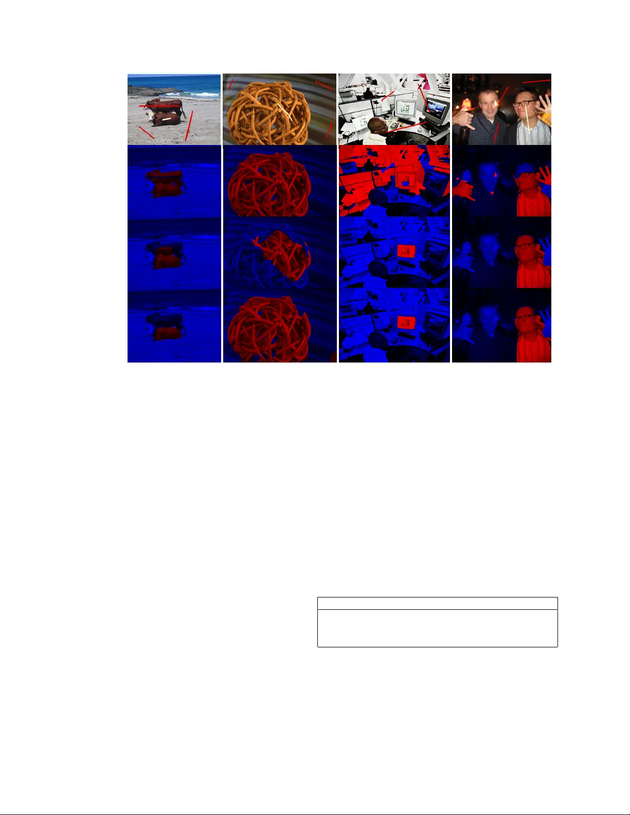
Authors: Alex, er Fix, Thorsten Joachims
Structur ed learning of sum-of-submodular higher order ener gy functions Alexander Fix Thorsten Joachims Sam Park Ramin Zabih Abstract Submodular functions can be exactly minimized in poly- nomial time , and the special case that graph cuts solve with max flow [ 18 ] has had significant impact in computer vi- sion [ 5 , 20 , 27 ]. In this paper we addr ess the important class of sum-of-submodular (SoS) functions [ 2 , 17 ], which can be efficiently minimized via a variant of max flow called submodular flow [ 6 ]. SoS functions can naturally expr ess higher or der priors involving , e.g ., local image patches; however , it is dif ficult to fully exploit their expr essive power because they have so many parameters. Rather than trying to formulate existing higher or der priors as an SoS func- tion, we take a discriminative learning appr oach, effectively sear ching the space of SoS functions for a higher or der prior that performs well on our training set. W e adopt a structural SVM appr oach [ 14 , 33 ] and formulate the train- ing pr oblem in terms of quadratic pr ogramming; as a re- sult we can efficiently sear ch the space of SoS priors via an extended cutting-plane algorithm. W e also show how the state-of-the-art max flow method for vision pr oblems [ 10 ] can be modified to efficiently solve the submodular flow pr oblem. Experimental comparisons ar e made against the OpenCV implementation of the GrabCut interactive seg- mentation technique [ 27 ], which uses hand-tuned parame- ters instead of machine learning. On a standard dataset [ 11 ] our method learns higher order priors with hundreds of parameter values, and pr oduces significantly better seg- mentations. While our focus is on binary labeling pr oblems, we show that our techniques can be naturally generalized to handle mor e than two labels. 1. Introduction Discrete optimization methods such as graph cuts [ 5 , 18 ] hav e prov en to be quite ef fecti ve for many computer vi- sion problems, including stereo [ 5 ], interactiv e segmenta- tion [ 27 ] and texture synthesis [ 20 ]. The underlying opti- mization problem behind graph cuts is a special case of sub- modular function optimization that can be solved exactly using max flow [ 18 ]. Graph cut methods, howe ver , are lim- ited by their reliance on first-order priors in volving pairs of pixels, and there is considerable interest in expressing priors that rely on local image patches such as the popular Field of Experts model [ 26 ]. In this paper we focus on an important generalization of the functions that graph cuts can minimize, which can express higher-order priors. These functions, which [ 17 ] called Sum-of-Submodular (SoS), can be efficiently solved with a v ariant of max flow [ 6 ]. While SoS functions ha ve more expressi ve power , they also in v olve a lar ge number of parameters. Rather than addressing the question of which existing higher order priors can be expressed as an SoS function, we take a discriminati ve learning approach and effecti vely search the space of SoS functions with the goal of finding a higher order prior that gives strong results on our training set. 1 Our main contribution is to introduce the first learning method for training such SoS functions, and to demonstrate the effecti veness of this approach for interactiv e se gmenta- tion using learned higher order priors. Follo wing a Struc- tural SVM approach [ 14 , 33 ], we show that the training problem can be cast as a quadratic optimization problem ov er an e xtended set of linear constraints. This generalizes large-mar gin training of pairwise submodular (a.k.a. re gular [ 18 ]) MRFs [ 1 , 29 , 30 ], where submodularity corresponds to a simple non-negati vity constraint. T o solve the training problem, we sho w that an e xtended cutting-plane algorithm can efficiently search the space of SoS functions. 1.1. Sum-of-Submodular functions and priors A submodular function f : 2 V → R on a set V satisfies f ( S ∩ T ) + f ( S ∪ T ) ≤ f ( S ) + f ( T ) for all S, T ⊆ V . Such a function is sum-of-submodular (SoS) if we can write it as f ( S ) = X C ∈C f C ( S ∩ C ) (1) for C ⊆ 2 V where each f C : 2 C → R is submodular . Re- search on higher-order priors calls C ∈ C a clique [ 13 ]. Of course, a sum of submodular functions is itself sub- modular , so we could use general submodular optimization to minimize an SoS function. Ho wev er, general submod- ular optimization is O ( n 6 ) [ 25 ] (which is impractical for 1 Since we are taking a discriminati ve approach, the higher-order en- ergy function we learn does not have a natural probabilistic interpretation. W e are using the word “prior” here somewhat loosely , as is common in computer vision papers that focus on energy minimization. 1 low-le vel vision problems), whereas we may be able to ex- ploit the neighborhood structure C to do better . F or exam- ple, if all the cliques are pairs ( | C | = 2 ) the energy function is referred to as regular and the problem can be reduced to max flow [ 18 ]. As mentioned above, this is the under- lying technique used in the popular graph cuts approach [ 5 , 20 , 27 ]. The key limitation is the restriction to pair- wise cliques, which does not allow us to naturally express important higher order priors such as those in volving im- age patches [ 26 ]. The most common approach to solving higher-order priors with graph cuts, which in volves trans- formation to pairwise cliques, in practice almost alw ays produces non-submodular functions that cannot be solved exactly [ 8 , 13 ]. 2. Related W ork Many learning problems in computer vision can be cast as structured output prediction, which allo ws learning out- puts with spatial coherence. Among the most popular generic methods for structured output learning are Condi- tional Random Fields (CRFs) trained by maximum con- ditional likelihood [ 22 ], Maximum-Margin Marko v Net- works (M3N) [ 32 ], and Structural Support V ector Machines (SVM-struct) [ 33 , 14 ]. A key advantage of M3N and SVM- struct over CRFs is that training does not require computa- tion of the partition function. Among the two large-mar gin approaches M3N and SVM-struct, we follow the SVM- struct methodology since it allows the use of efficient in- ference procedures during training. In this paper , we will learn submodular discriminant functions. Prior work on learning submodular functions falls into three categories: submodular function regression [ 3 ], maximization of submodular discriminant functions, and minimization of submodular discriminant functions. Learning of submodular discriminant functions where a prediction is computed through maximization has widespread use in information retriev al, where submodu- larity models div ersity in the ranking of a search engine [ 34 , 23 ] or in an automatically generated abstract [ 28 ]. While e xact (monotone) submodular maximization is in- tractible, approximate inference using a simple greedy algo- rithm has approximation guarantees and generally e xcellent performance in practice. The models considered in this paper use submodular dis- criminant functions where a prediction is computed through minimization. The most popular such models are regular MRFs [ 18 ]. Traditionally , the parameters of these mod- els have been tuned by hand, b ut sev eral learning methods exist. Most closely related to the work in this paper are Associativ e Markov Networks [ 30 , 1 ], which take an M3N approach and exploit the fact that regular MRFs have an integral linear relaxation. These linear programs (LP) are folded into the M3N quadratic program (QP) that is then solved as a monolithic QP . In contrast, SVM-struct train- ing using cutting planes for regular MRFs [ 29 ] allows graph cut inference also during training, and [ 7 , 19 ] sho w that this approach has interesting approximation properties even the for multi-class case where graph cut inference is only ap- proximate. More comple x models for learning spatially co- herent priors include separate training for unary and pair- wise potentials [ 21 ], learning MRFs with functional gradi- ent boosting [ 24 ], and the P n Potts models, all of which hav e had success on a variety of vision problems. Note that our general approach for learning multi-label SoS functions, described in section 4.4 , includes the P n Potts model as a special case. 3. SoS minimization In this section, we briefly summarize how an SoS func- tion can be minimized by means of a submodular flow net- work (section 3.1 ), and then present our improv ed algorithm for solving this minimization (section 3.2 ). 3.1. SoS minimization via submodular flow Submodular flow is similar to the max flo w problem, in that there is a network of nodes and arcs on which we want to push flow from s to t . Howe ver , the notion of residual capacity will be slightly modified from that of standard max flow . F or a much more complete description see [ 17 ]. W e begin with a network G = ( V ∪ { s, t } , A ) . As in the max flo w reduction for Graph Cuts, there are source and sink arcs ( s, i ) and ( i, t ) for every i ∈ V . Additionally , for each clique C , there is an arc ( i, j ) C for each i, j ∈ C . 2 Every arc a ∈ A also has an associated residual capac- ity c a . The residual capacity of arcs ( s, i ) and ( i, t ) are the familiar residual capacities from max flow: there are capac- ities c s,i and c i,t (determined by the unary terms of f ), and whenev er we push flo w on a source or sink arc, we decrease the residual capacity by the same amount. For the interior arcs, we need one further piece of in- formation. In addition to residual capacities, we also keep track of residual clique functions f C ( S ) , related to the flo w values by the following rule: whene ver we push δ units of flow on arc ( i, j ) C , we update f C ( S ) by f C ( S ) ← f C ( S ) − δ i ∈ S, j / ∈ S f C ( S ) + δ i / ∈ S, j ∈ S f C ( S ) otherwise (2) The residual capacities of the interior arcs are chosen so that the f C are always nonnegati ve. Accordingly , we define c i,j,C = min S { f C ( S ) | i ∈ S, j / ∈ S } . 2 T o explain the notation, note that i, j might be in multiple cliques C , so we may ha ve multiple edges ( i, j ) (that is, G is a multigraph). W e distinguish between them by the subscript C . Giv en a flow φ , define the set of residual arcs A φ as all arcs a with c a > 0 . An augmenting path is an s − t path along arcs in A φ . The following theorem of [ 17 ] tells how to optimize f by computing a flow in G . Theorem 3.1. Let φ be a feasible flow such that ther e is no augmenting path fr om s to t . Let S ∗ be the set of all i ∈ V reac hable fr om s along ar cs in A φ . Then f ( S ∗ ) is the minimum value of f over all S ⊆ V . 3.2. IBFS f or Submodular Flow Incremental Breadth First Search (IBFS) [ 10 ], which is the state of the art in max flow methods for vision appli- cations, improves the algorithm of [ 4 ] to guarantee polyno- mial time complexity . W e no w sho w ho w to modify IBFS to compute a maximum submodular flow in G . IBFS is an augmenting paths algorithm: at each step, it finds a path from s to t with positiv e residual capacity , and pushes flow along it. Additionally , each augmenting path found is a shortest s - t path in A φ . T o ensure that the paths found are shortest paths, we keep track of distances d s ( i ) and d t ( i ) from s to i and from i to t , and search trees S and T containing all nodes at distance at most D s from s or D t from t respectiv ely . T wo in variants are maintained: • For every i in S , the unique path from s to i in S is a shortest s - i path in A φ . • For every i in T , the unique path from i to t in T is a shortest i - t path in A φ . The algorithm proceeds by alternating between forward passes and reverse passes. In a forward pass, we attempt to grow the source tree S by one layer (a re verse pass attempts to grow T , and is symmetric). T o gro w S , we scan through the vertices at distance D s away from s , and examine each out-arc ( i, j ) with positi ve residual capacity . If j is not in S or T , then we add j to S at distance lev el D s + 1 , and with parent i . If j is in T , then we found an augmenting path from s to t via the arc ( i, j ) , so we can push flow on it. The operation of pushing flow may saturate some arcs (and cause previously saturated arcs to become unsatu- rated). If the parent arc of i in the tree S or T becomes saturated, then i becomes an orphan. After each augmenta- tion, we perform an adoption step, where each orphan finds a ne w parent. The details of the adoption step are similar to the relabel operation of the Push-Relabel algorithm, in that we search all potential parent arcs in A φ for the neighbor with the lowest distance label, and make that node our new parent. In order to apply IBFS to the submodular flo w problem, all the basic datastructures still make sense: we have a graph where the arcs a have residual capacities c a , and a maxi- mum flo w has been found if and only if there is no longer any augmenting path from s to t . The main change for the submodular flow problem is that when we increase flo w on an edge ( i, j ) C , instead of just af- fecting the residual capacity of that arc and the re verse arc, we may also change the residual capacities of other arcs ( i 0 , j 0 ) C for i 0 , j 0 ∈ C . Howe ver , the following result en- sures that this is not a problem. Lemma 3.2. If ( a, b ) C was pr eviously saturated, but now has r esidual capacity as a result of incr easing flow along ( c, d ) , then (1) either a = d or ther e was an ar c ( a, d ) ∈ A φ and (2) either b = c or ther e was an arc ( c, b ) ∈ A φ . Corollary 3.3. Increasing flow on an edge never cr eates a shortcut between s and i , or fr om i to t . The proofs are based on results of [ 9 ], and can be found in the Supplementary Material. Corollary 3.3 ensures that we nev er create any new shorter s - i or i - t paths not contained in S or T . A push operation may cause some edges to become saturated, but this is the same problem as in the normal max flow case, and an y orpans so created will be fix ed in the adoption step. Therefore, all in variants of the IBFS algorithm are main- tained, ev en in the submodular flow case. One final property of the IBFS algorithm in volves the use of the “current arc heuristic”, which is a mechanism for av oiding iterating through all possible potential parents when performing an adoption step. In the case of Submod- ular Flows, it is also the case that whene ver we create ne w residual arcs we maintain all inv ariants related to this cur - rent arc heuristic, so the same speedup applies here. How- ev er, as this does not af fect the correctness of the algorithm, and only the runtime, we will defer the proof to the Supple- mentary Material. Running time. The asymptotic complexity of the stan- dard IBFS algorithm is O ( n 2 m ) . In the submodular-flo w case, we still perform the same number of basic operations. Howe ver , note finding residual capacity of an arc ( i, j ) C requires minimizing f C ( S ) for S separating i and j . If | C | = k , this can be done in time O ( k 6 ) using [ 25 ]. How- ev er, for k << n , it will likely be much more efficient to use the O (2 k ) naiv e algorithm of searching through all values of f C . Overall, we add O (2 k ) work at each basic step of IBFS, so if we hav e m cliques the total runtime is O ( n 2 m 2 k ) . This runtime is better than the augmenting paths algo- rithm of [ 2 ] which takes time O ( nm 2 2 k ) . Additionally , IBFS has been shown to be very f ast on typical vision in- puts, independent of its asymptotic complexity [ 10 ]. 4. S3SVM: SoS Structured SVMs In this section, we first revie w the SVM algorithm and its associated Quadratic Program (section 4.1 ). W e then de- cribe a general class of SoS discriminant functions which can be learned by SVM-struct (section 4.2 ) and e xplain this learning procedure (section 4.3 ). Finally , we generalize SoS functions to the multi-label case (section 4.4 ). 4.1. Structured SVMs Structured output prediction describes the problem of learning a function h : X − → Y where X is the space of inputs, and Y is the space of (multiv ariate and struc- tured) outputs for a given problem. T o learn h , we as- sume that a training sample of input-output pairs S = (( x 1 , y 1 ) , . . . , ( x n , y n )) ∈ ( X × Y ) n is av ailable and drawn i.i.d. from an unknown distribution. The goal is to find a function h from some hypothesis space H that has low prediction error , relative to a loss function ∆( y , ¯ y ) . The function ∆ quantifies the error associated with predicting ¯ y when y is the correct output v alue. For example, for image segmentation, a natural loss function might be the Hamming distance between the true segmentation and the predicted la- beling. The mechanism by which Structural SVMs finds a hy- pothesis h is to learn a discriminant function f : X ×Y → R ov er input/output pairs. One deriv es a prediction for a given input x by minimizing f over all y ∈ Y . 3 W e will write this as h w ( x ) = argmin y ∈Y f w ( x, y ) . W e assume f w ( x, y ) is linear in two quantities w and Ψ f w ( x, y ) = w T Ψ( x, y ) where w ∈ R N is a parameter vector and Ψ( x, y ) is a fea- ture vector relating input x and output y . Intuitiv ely , one can think of f w ( x, y ) as a cost function that measures ho w poorly the output y matches the giv en input x . Ideally , we would find weights w such that the hypothe- sis h w always gi ves correct results on the training set. Stated another way , for each example x i , the correct prediction y i should hav e low discriminant v alue, while incorrect predic- tions ¯ y i with lar ge loss should ha ve high discriminant val- ues. W e write this constraint as a linear inequality in w w T Ψ( x i , ¯ y i ) ≥ w T Ψ( x i , y i ) + ∆( y i , ¯ y i ) : ∀ ¯ y ∈ Y . (3) It is con venient to define δ Ψ i ( ¯ y ) = Ψ( x i , ¯ y ) − Ψ( x i , y i ) , so that the abov e inequality becomes w T δ Ψ i ( ¯ y i ) ≥ ∆( y i , ¯ y i ) . Since it may not be possible to satisfy all these condi- tions exactly , we also add a slack v ariable to the constraints for example i . Intuiti vely , slack variable ξ i represents the maximum misprediction loss on the i th example. Since we want to minimize the prediction error , we add an objectiv e function which penalizes large slack. Finally , we also pe- nalize k w k 2 to discourage overfitting, with a regularization parameter C to trade of f these costs. Quadratic Program 1. n - S L AC K S T RU C T U R A L S V M 3 Note that the use of minimization departs from the usual language of [ 33 , 14 ] where the hypothesis is argmax f w ( x, y ) . Ho wever , because of the prev alence of cost functions throughout computer vision, we have replaced f by − f throughout. min w ,ξ ≥ 0 1 2 w T w + C n n X i =1 ξ i ∀ i, ∀ ¯ y i ∈ Y : w T δ Ψ i ( ¯ y i ) ≥ ∆( y i , ¯ y i ) − ξ i 4.2. Submodular F eature Encoding W e now apply the Structured SVM (SVM-struct) frame- work to the problem of learning SoS functions. For the moment, assume our prediction task is to assign a binary label for each element of a base set V . W e will cov er the multi-label case in section 4.4 . Since the labels are binary , prediction consists of assigning a subset S ⊆ V for each input (namely the set S of pix els labeled 1). Our goal is to construct a feature vector Ψ that, when used with the SVM-struct algorithm of section 4.1 , will al- low us to learn sum-of-submodular energy functions. Let’ s begin with the simplest case of learning a discriminant func- tion f C, w ( S ) = w T Ψ( S ) , defined only on a single clique and which does not depend on the input x . Intuitiv ely , our parameters w will correspond to the table of v alues of the clique function f C , and our feature v ector Ψ will be chosen so that w S = f C ( S ) . W e can accomplish this by letting Ψ and w hav e 2 | C | entries, index ed by subsets T ⊆ C , and defining Ψ T ( S ) = δ T ( S ) (where δ T ( S ) is 1 if S = T and 0 otherwise). Note that, as we claimed, f C, w ( S ) = w T Ψ( S ) = X T ⊆ C w T δ T ( S ) = w S . (4) If our parameters w T are allowed to vary ov er all R 2 | C | , then f C ( S ) may be an arbitrary function 2 C → R , and not necessarily submodular . Howe ver , we can enforce submod- ularity by adding a number of linear inequalities. Recall that f is submodular if and only if f ( A ∪ B ) + f ( A ∩ B ) ≤ f ( A ) + f ( B ) . Therefore, f C, w is submodular if and only if the parameters satisfy w A ∪ B + w A ∩ B ≤ w A + w B : ∀ A, B ⊆ C (5) These are just linear constraints in w , so we can add them as additional constraints to Quadratic Program 1 . There are O (2 | C | ) of them, b ut each clique has 2 | C | parameters, so this does not increase the asymptotic size of the QP . Theorem 4.1. By choosing featur e vector Ψ T ( S ) = δ T ( S ) and adding the linear constr aints ( 5 ) to Quadratic Pr o- gram 1 , the learned discriminant function f w ( S ) is the max- imum mar gin function f C , wher e f C is allowed to vary over all possible submodular functions f : 2 C → R . Pr oof. By adding constraints ( 5 ) to the QP , we ensure that the optimal solution w is defines a submodular f w . Con- versely , for any submodular function f C , there is a feasible w defined by w T = f C ( T ) , so the optimal solution to the QP must be the maximum-margin such function. Algorithm 1 : S3SVM via the 1 -Slack F ormulation. 1: Input: S = (( x 1 , y 1 ) , . . . , ( x n , y n )) , C , 2: W ← ∅ 3: r epeat 4: Recompute the QP solution with the current con- straint set: ( w , ξ ) ← argmin w ,ξ ≥ 0 1 2 w T w + C ξ s.t. for all ( ¯ y 1 , . . . , ¯ y n ) ∈ W : 1 n w T P n i =1 δ Ψ i ( ¯ y i ) ≥ 1 n P n i =1 ∆( y i , ¯ y i ) − ξ s.t. for all C ∈ C , A, B ⊆ C : w C,A ∪ B + w C,A ∩ B ≤ w C,A + w C,B 5: f or i=1,...,n do 6: Compute the maximum violated constraint: ˆ y i ← argmin ˆ y ∈Y { w T Ψ( x i , ˆ y ) − ∆( y i , ˆ y ) } by using IBFS to minimize f w ( x i , ˆ y ) − ∆( y i , ˆ y ) . 7: end f or 8: W ← W ∪ { ( ˆ y 1 , . . . , ˆ y n ) } 9: until the slack of the max-violated constraint is ≤ ξ + . 10: r eturn ( w , ξ ) T o introduce a dependence on the data x , we can define Ψ data to be Ψ data T ( S, x ) = δ T ( S )Φ( x ) for an arbitrary non- negati ve function Φ : X → R ≥ 0 . Corollary 4.2. W ith featur e vector Ψ data and adding linear constraints ( 5 ) to QP 1 , the learned discriminant function is the maximum mar gin function f C ( S )Φ( x ) , wher e f C is allowed to vary over all possible submodular functions. Pr oof. Because Φ( x ) is nonneg ati ve, constraints ( 5 ) ensure that the discriminant function is again submodular . Finally , we can learn multiple clique potentials simul- taneously . If we have a neighborhood structure C with m cliques, each with a data-dependence Φ C ( x ) , we create a feature vector Ψ sos composed of concatenating the m dif- ferent features Ψ data C . Corollary 4.3. W ith featur e vector Ψ sos , and adding a copy of the constraints ( 5 ) for each clique C , the learned f w is the maximum mar gin f of the form f ( x, S ) = X C ∈C f C ( S )Φ C ( x ) (6) wher e the f C can vary over all possible submodular func- tions on the cliques C . 4.3. Solving the quadratic program The n -slack formulation for SSVMs (QP 1 ) makes intu- itiv e sense, from the point of view of minimizing the mis- prediction error on the training set. Howe ver , in practice it is better to use the 1 -slack reformulation of this QP from [ 14 ]. Compared to n -slack, the 1 -slack QP can be solved sev eral orders of magnitude faster in practice, as well as having asymptotically better comple xity . The 1 -slack formulation is an equiv alent QP which re- places the n slack variables ξ i with a single variable ξ . The loss constraints ( 3 ) are replaced with constraints penalizing the sum of losses across all training examples. W e also in- clude submodular constraints on w . Quadratic Program 2. 1 - S L AC K S T RU C T U R A L S V M min w ,ξ ≥ 0 1 2 w T w + C ξ s.t. ∀ ( ¯ y 1 , ..., ¯ y n ) ∈ Y n : 1 n w T n X i =1 δ Ψ i ( ¯ y i ) ≥ 1 n n X i =1 ∆( y i , ¯ y i ) − ξ ∀ C ∈ C , A, B ⊆ C : w C,A ∪ B + w C,A ∩ B ≤ w C,A + w C,B Note that we have a constraint for each tuple ( ¯ y 1 , . . . , ¯ y n ) ∈ Y n , which is an exponential sized set. De- spite the large set of constraints, we can solve this QP to any desired precision by using the cutting plane algorithm. This algorithm k eeps track of a set W of current constraints, solves the current QP with re gard to those constraints, and then giv en a solution ( w , ξ ) , finds the most violated con- straint and adds it to W . Finding the most violated con- straint consists of solving for each example x i the problem ˆ y i = argmin ˆ y ∈Y f w ( x, ˆ y ) − ∆( y i , ˆ y ) . (7) Since the features Ψ ensure that f w is SoS, then as long as ∆ factors as a sum o ver the cliques C (for instance, the Ham- ming loss is such a function), then ( 7 ) can be solved with Submodular IBFS. Note that this also allo ws us to add arbi- trary additional features for learning the unary potentials as well. Pseudocode for the entire S3SVM learning is giv en in Algorithm 1 . 4.4. Generalization to multi-label prediction Submodular functions are intrinsically binary functions. In order to handle the multi-label case, we use expansion mov es [ 5 ] to reduce the multi-label optimization problem to a series of binary subproblems, where each pixel may either switch to a giv en label α or keep its current label. If ev ery binary subproblem of computing the optimal ex- pansion mo ve is an SoS problem, we will call the original multi-label energy function an SoS e xpansion energy . Let L be our label set, with output space Y = L V . Our learned function will have the form f ( y ) = P C ∈C f C ( y C ) where f C : L C → R . For a clique C and label ` , define C ` = { i | y i = ` } , i.e., the subset of C taking label ` . Theorem 4.4. If all the clique functions are of the form f C ( y C ) = X ` ∈ L g ` ( C ` ) (8) wher e each g ` is submodular , then any expansion move for the multi-label ener gy function f will be SoS. Figure 1. Example images from the binary segmentation results. From left to right, the columns are (a) the original image (b) the noisy input (c) results from Generic Cuts [ 2 ] (d) our results. Pr oof. Fix a current labeling y , and let B ( S ) be the energy when the set S switches to label α . W e can write B ( S ) in terms of the clique functions and sets C ` as B ( S ) = X C ∈C g α ( C α ∪ S ) + X ` 6 = α g ` ( C ` \ S ) (9) W e use a fact from the theory of submodular functions: if f ( S ) is submodular , then for any fixed T both f ( T ∪ S ) and f ( T \ S ) are also submodular . Therefore, B ( S ) is SoS. Theorem 4.4 characterizes a large class of SoS expan- sion energies. These functions generalize commonly used multi-label clique functions, including the P n Potts model [ 15 ]. The P n model pays cost λ i when all pixels are equal to label i , and λ max otherwise. W e can write this as an SoS expansion energy by letting g ` ( S ) = λ i − λ max if S = C and otherwise 0 . Then, P ` g ` ( S ) is equal to the P n Potts model, up to an additi ve constant. Generalizations such as the robust P n model [ 16 ] can be encoded in a similar fash- ion. Finally , in order to learn these functions, we let Ψ be composed of copies of Ψ data — one for each g ` , and add corresponding copies of the constraints ( 5 ). As a final note: even though the indi vidual expansion mov es can be computed optimally , α -expansion still may not find the global optimum for the multi-labeled energy . Howe ver , in practice α -e xpansion finds good local optima, and has been used for inference in Structural SVM with good results, as in [ 19 ]. 5. Experimental Results In order to ev aluate our algorithms, we focused on binary denoising and interactive segmentation. For binary denois- ing, Generic Cuts [ 2 ] provides the most natural comparison since it is a state-of-the-art method that uses SoS priors. F or interactiv e segmentation the natural comparison is against GrabCut [ 27 ], where we used the OpenCV implementation. W e ran our general S3SVM method, which can learn an arbitrary SoS function, an also considered the special case of only using pairwise priors. For both the denoising and segmentation applications, we significantly improve on the accuracy of the hand-tuned ener gy functions. 5.1. Binary denoising Our binary denoising dataset consists of a set of 20 black and white images. Each image is 400 × 200 and either a set of geometric lines, or a hand-drawn sketch (see Fig- ure 1 ). W e were unable to obtain the original data used by [ 2 ], so we created our own similar data by adding indepen- dent Gaussian noise at each pixel. For denoising, the hand-tuned Generic Cuts algorithm of [ 2 ] posed a simple MRF , with unary pixels equal to the absolute v alued distance from the noisy input, and an SoS prior , where each 2 × 2 clique penalizes the square-root of the number of edges with different labeled endpoints within that clique. There is a single parameter λ , which is the tradeoff between the unary energy and the smoothness term. The neighborhood structure C consists of all 2 × 2 patches of the image. Our learned prior includes the same unary terms and clique structure, but instead of the square-root smooth- ness prior , we learn a clique function g to get an MRF E SVM ( y ) = P i | y i − x i | + P C ∈C g ( y C ) . Note that each clique has the same energy as ev ery other, so this is anal- ogous to a graph cuts prior where each pairwise edge has the same attractive potential. Our energy function has 16 total parameters (one for each possible value of g , which is defined on 2 × 2 patches). W e randomly di vided the 20 input images into 10 train- ing images and 10 test images. The loss function was the Hamming distance between the correct, un-noisy image and the predicted image. T o hand tune the value λ , we picked the value which gave the minimum pixel-wise error on the training set. S3SVM training took only 16 minutes. Numerically , S3SVM performed signficantly better than the hand-tuned method, with an average pixel-wise error of only 4.9% on the training set, compared to 28.6% for Generic Cuts. The time needed to do inference after training was similar for both methods: 0.82 sec/image for S3SVM vs. 0.76 sec/image for Generic Cuts. V isually , the S3SVM images are significantly cleaner looking, as shown in Fig- ure 1 . 5.2. Interactive segmentation The input to interacti ve segmentation is a color image, together with a set of sparse foreground/background anno- tations provided by the user . See Figure 2 for examples. From the small set of labeled foreground and background pixels, the prediction task is to recov er the ground-truth seg- mentation for the whole image. Our baseline comparison is the Grabcut algorithm, which solves a pairwise CRF . The unary terms of the CRF are obtained by fitting a Gaussian Mixture Model to the his- tograms of pixels labeled as being definitely foreground or background. The pairwise terms are a standard contrast- sensitiv e Potts potential, where the cost of pixels i and j Input GrabCut S3SVM-AMN S3SVM Figure 2. Example images from binary segmentation results. Input with user annotations are shown at top, with results belo w . taking different labels is equal to λ · exp ( − β | x i − x j | ) for some hand-coded parameters β , λ . Our primary comparison is against the OpenCV implementation of Grabcut, av ail- able at www.opencv.org . As a special case, our algorithm can be applied to pairwise-submodular energy functions, for which it solves the same optimization problem as in Associativ e Markov Networks (AMN’ s) [ 30 , 1 ]. Automatically learning param- eters allo ws us to add a large number of learned unary fea- tures to the CRF . As a result, in addition to the smoothness parameter λ , we also learn the relativ e weights of approximately 400 features describing the color v alues near a pixel, and rela- tiv e distances to the nearest labeled foreground/background pixel. Further details on these features can be found in the Supplementary Material. W e refer to this method as S3SVM-AMN. Our general S3SVM method can incorporate higher- order priors instead of just pairwise ones. In addition to the unary features used in S3SVM-AMN, we add a sum- of-submodular higher-order CRF . Each 2 × 2 patch in the image has a learned submodular clique function. T o ob- tain the benefits of the contrast-sensiti ve pairwise potentials for the higher-order case, we cluster (using k -means) the x and y gradient responses of each patch into 50 clusters, and learn one submodular potential for each cluster . Note that S3SVM automatically allo ws learning the entire energy function, including the clique potentials and unary poten- tials (which come from the data) simultaneously . W e use a standard interactive segmentation dataset from [ 11 ] of 151 images with annotations, together with pixel- lev el segmentations provided as ground truth. These im- ages were randomly sorted into training, validation and test- ing sets, of size 75, 38 and 38 respectively . W e trained both S3SVM-AMN and S3SVM on the training set for v ar- ious v alues of the re gularization parameter c , and picked the value c which ga ve the best accurac y on the validation set, and report the results of that value c on the test set. The ov erall performance is shown in the table belo w . T raining time is measured in seconds, and testing time in seconds per image. Our implementation, which used the submodular flow algorithm based on IBFS discussed in sec- tion 3.2 , will be made freely available under the MIT li- cense. Algorithm A verage err or T raining T esting Grabcut 10.6 ± 1.4% n/a 1.44 S3SVM-AMN 7.5 ± 0.5% 29000 0.99 S3SVM 7.3 ± 0.5% 92000 1.67 Learning and validation was performed 5 times with in- dependently sampled training sets. The averages and stan- dard deviations sho wn above are from these 5 samples. While our focus is on binary labeling problems, we ha ve conducted some preliminary experiments with the multi- label version of our method described in section 4.4 . A Figure 3. A multi-label segmentation result, on data from [ 12 ]. The purple label represents vegetation, red is rhino/hippo and blue is ground. There are 7 labels in the input problem, though only 3 are present in the output we obtain on this particular image. sample result is sho wn in figure 3 , using an image taken the Corel dataset used in [ 12 ]. References [1] D. Anguelov , B. T askar , V . Chatalbashev , D. K oller , D. Gupta, G. Heitz, and A. Y . Ng. Discriminati ve learning of Mark ov Random Fields for segmentation of 3D scan data. In CVPR , 2005. 1 , 2 , 7 [2] C. Arora, S. Banerjee, P . Kalra, and S. N. Maheshwari. Generic cuts: an efficient algorithm for optimal inference in higher order MRF-MAP. In ECCV , 2012. 1 , 3 , 6 [3] M.-F . Balcan and N. J. A. Harvey . Learning submodular functions. In STOC , 2011. 2 [4] Y . Boyko v and V . K olmogorov . An e xperimental comparison of min-cut/max-flow algorithms for energy minimization in vision. TP AMI , 26(9), 2004. 3 [5] Y . Boykov , O. V eksler , and R. Zabih. Fast approximate en- ergy minimization via graph cuts. TP AMI , 23(11), 2001. 1 , 2 , 5 [6] J. Edmonds and R. Giles. A min-max relation for submod- ular functions on graphs. Annals of Discr ete Mathematics , 1:185–204, 1977. 1 [7] T . Finley and T . Joachims. T raining structural SVMs when exact inference is intractable. In ICML , 2008. 2 [8] A. Fix, A. Gruber, E. Boros, and R. Zabih. A graph cut algorithm for higher-order Marko v Random Fields. In ICCV , 2011. 2 [9] S. Fujishige and X. Zhang. A push/relabel framework for submodular flows and its refinement for 0-1 submodular flows. Optimization , 38(2):133–154, 1996. 3 [10] A. V . Goldberg, S. Hed, H. Kaplan, R. E. T arjan, and R. F . W erneck. Maximum flows by incremental breadth-first search. In Eur opean Symposium on Algorithms , 2011. 1 , 3 [11] V . Gulshan, C. Rother , A. Criminisi, A. Blak e, and A. Zis- serman. Geodesic star con vexity for interactiv e image seg- mentation. In CVPR , 2010. 1 , 7 [12] X. He, R. S. Zemel, and M. A. Carreira-Perpi ˜ n ´ an. Multi- scale conditional random fields for image labeling. In CVPR , 2004. 7 , 8 [13] H. Ishikawa. T ransformation of general binary MRF mini- mization to the first order case. TP AMI , 33(6), 2010. 1 , 2 [14] T . Joachims, T . Finley , and C.-N. Y u. Cutting-plane training of structural SVMs. Machine Learning , 77(1), 2009. 1 , 2 , 4 , 5 [15] P . Kohli, M. P . Kumar , and P . H. T orr . P3 and beyond: Mov e making algorithms for solving higher order functions. TP AMI , 31(9), 2008. 6 [16] P . Kohli, L. Ladick y , and P . T orr . Robust higher order poten- tials for enforcing label consistency . IJCV , 82, 2009. 6 [17] V . K olmogorov . Minimizing a sum of submodular functions. Discr ete Appl. Math. , 160(15):2246–2258, Oct. 2012. 1 , 2 [18] V . K olmogorov and R. Zabih. What ener gy functions can be minimized via graph cuts? TP AMI , 26(2), 2004. 1 , 2 [19] H. K oppula, A. Anand, T . Joachims, and A. Saxena. Seman- tic labeling of 3D point clouds for indoor scenes. In NIPS , 2011. 2 , 6 [20] V . Kwatra, A. Schodl, I. Essa, G. T urk, and A. Bobick. Graphcut textures: Image and video synthesis using graph cuts. SIGGRAPH , 2003. 1 , 2 [21] L. Ladicky , C. Russell, P . Kohli, and P . H. S. T orr . Associa- tiv e hierarchical CRFs for object class image segmentation. In ICCV , 2009. 2 [22] J. Lafferty , A. McCallum, and F . Pereira. Conditional ran- dom fields: Probabilistic models for se gmenting and labeling sequence data. In ICML , 2001. 2 [23] H. Lin and J. Bilmes. Learning mixtures of submodular shells with application to document summarization. In UAI , 2012. 2 [24] D. Munoz, J. A. Bagnell, N. V andapel, and M. Hebert. Con- textual classification with functional max-margin Markov networks. In CVPR , 2009. 2 [25] J. B. Orlin. A faster strongly polynomial time algorithm for submodular function minimization. Math. Pr ogram. , 118(2):237–251, Jan. 2009. 1 , 3 [26] S, Roth and M, Black. Fields of experts. IJCV , 82, 2009. 1 , 2 [27] C. Rother , V . K olmogorov , and A. Blake. “GrabCut” - inter- activ e foreground extraction using iterated graph cuts. SIG- GRAPH , 23(3):309–314, 2004. 1 , 2 , 6 [28] R. Sipos, P . Shiv aswamy , and T . Joachims. Large-margin learning of submodular summarization models. In EACL , 2012. 2 [29] M. Szummer , P . K ohli, and D. Hoiem. Learning CRFs using graph cuts. In ECCV , 2008. 1 , 2 [30] B. T askar , V . Chatalbashev , and D. K oller . Learning associa- tiv e markov networks. In ICML , 2004. 1 , 2 , 7 [31] B. T askar , V . Chatalbashev , and D. K oller . Learning associa- tiv e markov networks. In ICML . A CM, 2004. [32] B. T askar, C. Guestrin, and D. Koller . Maximum-margin markov netw orks. In NIPS , 2003. 2 [33] I. Tsochantaridis, T . Hofmann, T . Joachims, and Y . Al- tun. Support vector machine learning for interdependent and structured output spaces. In ICML , 2004. 1 , 2 , 4 [34] Y . Y ue and T . Joachims. Predicting diverse subsets using structural SVMs. In ICML , 2008. 2
Original Paper
Loading high-quality paper...
Comments & Academic Discussion
Loading comments...
Leave a Comment