Calculation of Entailed Rank Constraints in Partially Non-Linear and Cyclic Models

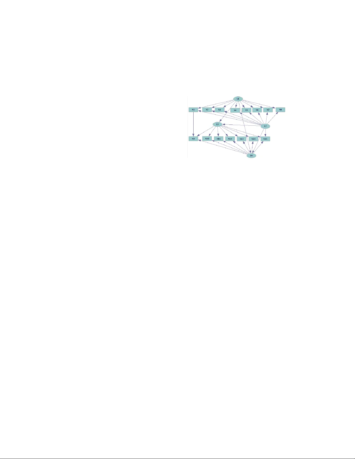
Calcul ation of En tail ed Rank Constr aints in Partially Non - Linear and Cyclic Model s Peter Spi rtes Depart ment o f Phi losop hy Carnegi e Mello n Univer sity p s7z@andrew .cmu.edu Abstract The Trek Separation T heorem (Sullivant et al. 2010) states necessary and sufficient co nditions for a linear directed acyclic graph ical mod el to entail for all possible values of its linear coefficients that the ran k of various sub - matrices of the covariance m atrix is less than or equal to n , for a ny given n . In this paper, I ex tend th e Trek S eparation Theorem in two way s: I prove that the same necess ary an d suffic ient con ditions apply even w hen the gen erating model is partially non - lin ear and contains so me cycles. This justifies application of constraint - based causal search algorithms to data generated by a wider clas s of caus al models that may contain non - linear and cyclic relations among the latent variables. 1 INTRODUCTION In m any cases, scientists are interested in infer ring causal relations between variables that ca nnot be d irectly measur ed (e.g. intelligence , anxiety , or impuls iveness) by administering test surveys wit h measure d “ indicators ” that indirectly measure the unmeasured or “ latent ” variables. In other cases, scientists are interested in estim ating the valu es of the latent variables from the measured indicators . The v ariances of the estimates of the latent variables of interest can be reduced in various ways by employ ing m ultiple indica tors for each latent variable. A model i n whic h each lat ent va riabl e of inter est is measur ed by multi ple indi cato rs (whic h may also be caused by other latents of interest as well as the error variable) is called a multiple indicator mode l . Multiple indictor models are quite common in many disciplines such as educational research, psychology, political science, etc. (Bartholomew et al., 2002) . Two major problems are how to use the values of the measur ed ind icat or var iabl es to make reliable infe rence s about the causal relatio nships between the latent variables of interest , and to pred ict the va lues of the la tent variables from the value s of the measured indicators. A number of c omplications make b oth of th ese tasks very dif ficul t: • Associ ation s among indicat ors are ofte n confounde d by additional unknown latent common causes; • One ind icat or may directly affe ct other indicators (e.g. “anchoring effe cts”); • There are often a plethora o f alternative causa l models that are consis tent with the data and with the prior knowledge of domain experts, often far too many mod els to t est indi vidual ly; • There may be non - line ar de pe ndencies among lat ent variables ; • There may be feedback relations hips a mong l aten t variables. The most common algori thms for using m easured indicators to find cau sal relations a mong latent variables or to i nfer the va lues of t he latent variables use some version of factor analysi s. However, given the models with the features cit ed above, factor analytic algorithms, as well as the FindHidden algori thm of Elidan (2001) have been shown to per form poorly (Silva et al. 2006) . One class of model search algorithms that hav e ha d som e success dealing with so me of the comp lications listed above is constraint - based search . A constra int - based search attempts to find the set o f mo dels that most closely match the measure d constraints on a probability distribution t hat are entail ed for all values of t he free parameters (e.g. conditional independence constraints that are entailed by d - separation) with constraints that are judged to hold in the populatio n (as determin ed by a statistical test). Althou gh mul tipl e indic ator models rar ely enta il any conditional independence constraints amo ng ju st th e measur ed indicators , multiple indicato r models often entail constraints on the rank of sub - matrices of the covariance matrix among the measured indicators (e.g. vanishing tetrad differences explained below ), and there are searches based on these rank c onstraints that have desirable proper ties (Silva et al. 2006) . Mult ipl e ind ica tor model s ar e spe cia l ca ses of stru ctur al equation models, and the fo rm o f the equations can be represented by a directed gra ph (Pearl 2000, Spirtes et al. 2001 ). Unde r the as sumpti on of lin earit y, the graphi cal structure representing the mul tipl e indicato r model can linearly enta il constraints on the covariance matrix of the variables, that is , constraints that hold for all values o f the fr ee parame ters (the lin ear co efficients associated with the edges, and the variances of the error terms). For ex ample, a multiple indicator model represented by a graph with a single latent variable L th at is the parent of measur ed indicators X , Y , Z , and W and contains no ot her edges , entails the vanishing tetrad difference (e .g. ρ ( X , Y ) ρ ( Z , W ) – ρ ( X , Z ) ρ ( Y , W ) = 0) for all valu es of the linear coefficients , w hich is e quivalent to a constraint that the rank of a sub matrix of the co variance matrix is less than or equal to 1. The T rek Separation Theorem (Sulliva nt et al. 2010) states necessary and sufficient conditions for a directed acyclic graph to linearly entail that the rank of various sub - matrice s of the covari ance matrix among the measur ed va riabl es a re l ess t han or eq ual t o n , for any n . The Trek Separa tion Theorem is one way to justify the correctness of the BuildP ureClust ers algorit hm (Silva et al. 2006) , that searches for the set of m ultiple indicator models that most close ly match the set of vanis hing tet rad differences judg ed to h old in th e population by application of statistical tests to the sample data. BuildPur eClust ers is a pointwise consistent algorithm that , depending upon the input data , either output s “Can’t tell” or an equivalence class of graphs that linearly entail the same set of vanishing tetrad differences and zero partial correlation constraint s. The al gorithm has been successfully applied to a num ber of data sets (Silva et al. 2006 , Jackson & Scheines 2005 ) However, there are a number of significa nt limi tations o n usefulness of the Trek Separation Theorem (and henc e on the BuildP ureClusters a lgorithm): • The Trek S eparati on T heorem does not apply to cyclic graphs (as in feedback models); • The Trek S eparati on Theorem does not apply if any of the causal relations bet ween the variables are non - linear . In this paper, I prove an extension of the trek separation theorem wh ich gives necessa ry and sufficient con ditions for a d irected graph (cy clic or acyclic) that has some functions relating variables to other variables t hat are non - linear, and in wh ich the re m ay be som e fee dback (represented by cyclic graphs) to entail th at the ra nk of various sub - matric es of th e covar iance matri x are le ss than or equal to n , fo r any n . This theorem has at least two uses for causal discover y : it serves as the basis for proving that existing algorithms for the linear case can be reliably applied to partially non - linear or cyclic models (described in s ection 4 ), and it could be used in the development of new algorithms for causal infer ence among models in which measured indicators have multi ple latent par ents but have non - linear or cyclic relations among th e latent parents. In section 2, I describe mu ltiple indicator models and the Trek Separat ion T heorem in more detail. In section 3, I state an extension of the trek sepa ration theorem that applies to graphs that m ay have cyclic and non - linear relationships am ong some variables. In section 4 , I discuss the issue of the ext ent to which it is to be expected that rank constraints on the covariance matrix m ight hold , or approximately hold , in the populat ion even if they are not entailed by the m odel to hold for all values of the free parameters of t he model. In section 5, I desc ribe open research questions. The Appendix cont ains t he proofs . 2 STRUCTURAL EQUATION MODELS In what follo ws, random variables are in italics, and sets of random variables are in boldf ace. . In a structural equation model ( SEM ) the random variables are divi ded into two disjoint set s, the substanti ve variables (typically the variables of interest) and the error variables (summarizing a ll oth er variables that have a causal influence on the substant ive variables) (Bollen, 1989) . Corr esponding to each substantive rando m variable V is a unique err or term ε V . A fixed pa rameter SEM S has two parts < φ , θ > , w here φ is a set of equations in w hich ea ch sub stantive random variab le V is w ritten a s a function of ot her substantive random variables and a unique error variable, together with θ , the joint distributions over the error variables . An example of a linear S EM is the ca se where φ contains the pair of linear equations X = 3 L + ε X , and L = ε L , and θ is a s tandardized Gaussi an distri butio n over ε X and ε L and ε X and ε L are independ ent. Together φ and θ determine a joint distribution over the substantive variables in S , which will be referred t o as the dist ribution entai led by S . A free para meter linear SEM m odel replaces som e o f the real numbe rs in the equ ations in φ with real - valued variables and a set of possible values for those variables, e.g . X = a X , L L + ε X , wher e a X , L can take on any real value. In addition, a free p arameter SEM can replace the particular distributi on over ε X and ε L with a parametric family of distributions, e.g. the bi - variate Gaussian distributions with zero covarianc e. T he free parameter SEM a lso has two parts < Φ , Θ >, where Φ contains the set of equations with free parameters and the set of values the free parame ters are allowed to take , and Θ is a family of distribut ions over the error variabl es. In gen eral, I will assume that there is a fini te set o f free parameters, and all allowed values of the free parameters lead to fix ed param eter SEM s that have a reduced form (i.e. each substantive variable X can be expressed as a function of the error variables of X and the error variables of its ancestors ), all variances and pa rtial variances am ong the substantiv e variables are fin ite and positive , a nd there are no deterministic relations among the m easured variables. The path diagram of a SEM with jointly independe nt errors is a directed graph, writte n with the convent ions that it co ntains an edge B → A if and only if B is a non - trivial arg ument of the equation for A . The error variables are not included in the path diagram. A fixed - parameter acyclic structural equa tion mo del (with out dou ble - headed arrows) is an instance of a B ayesian Network < G , P ( V )>, where the path diagram is G , an d P ( V ) is the joint distribution over the variables in G entailed by the set of equations and the joint distribution over the error var iables (P earl, 20 00; Sp irtes et al. 20 01 ). I t has been shown that wh en a directed cyclic graph is used to represent non - linear structu ral equations, then d - separation between A and B conditional on C does not entail the corresponding cond itional independence . E ven in non - linear cy clic structural equation models, if A and B are d - separated conditional on the emp ty set, the n A and B are entailed to be independent (Spirtes , 1995) , and that is the only feature of cyclic graphs th at the proofs below depend upon. A pol ynomial equation Q on the entries of a covariance (or correlation) m atrix C holds when C is a solution to Q . A polynomial Q is entailed by a free parameter SEM when all v alues of the free parameters entail covariance matri ces t hat are solut ions to Q . For example, a v anishing tetrad difference among { X , W } and { Y , Z }, w hich hold s if ρ ( X ,Y) ρ ( Z , W ) – ρ ( X , Z ) ρ ( Y , W ) = 0 , is entailed by a free p arameter SEM S in which X , Y , Z , and W are all children of just one latent variable L since any value of the free parameters in S entails a covariance matri x that is a solution to ρ ( X ,Y) ρ ( Z , W ) – ρ ( X , Z ) ρ ( Y , W ) = 0 . The following defini tions are illustr ated in Figure 1. A trek in G from I to J is an ord ered pair of directed path s ( P 1 ; P 2 ) where P 1 has sink I , P 2 has sink J , a nd both P 1 and P 2 have the same source k (e.g. (< L 1 , X 1 >;< L 1 , X 2 >) . The common source k is called the top of the trek, denoted top ( P 1 ; P 2 ) (e.g. top(< L 1 , X 1 >;< L 1 , X 2 >) is L 1 ). Note that one or both of P 1 and P 2 may consist of a single vertex, i.e., a path with no edges. A trek ( P 1 ; P 2 ) is simple if the only commo n vertex betw een P 1 and P 2 is the common source top ( P 1 ; P 2 ). Let A , B , be two di sjoint subsets of vertices V in G . L et T ( A , B ) and S ( A , B ) denote the sets of all tre ks and all sim ple treks from a memb er of A to a member of B , respectively. For exam ple, if A = { X 1 } and B = { X 2 }, S ( A , B ) = {(< L 1 , X 1 >;< L 1 , X 2 >) ; (< L 2 , X 1 >;< L 2 , X 2 >)}. For two sets of variables A and B , and a covariance or correlatio n matrix over a set of variables V containing A and B , let cov( A , B ) be the sub - matrix of Σ that contains the rows in A and columns in B . For e xample, if A = { X 1 , X 2 , X 3 }, and B = { X 4 , X 5 , X 10 }, then X 4 X 5 X 10 c ov( A , B ) = X 1 X 2 X 3 ρ ( X 1 , X 4 ) ρ ( X 1 , X 5 ) ρ ( X 1 , X 10 ) ρ ( X 2 , X 4 ) ρ ( X 2 , X 5 ) ρ ( X 2 , X 10 ) ρ ( X 3 , X 4 ) ρ ( X 3 , X 5 ) ρ ( X 3 , X 10 ) ⎡ ⎣ ⎢ ⎢ ⎢ ⎤ ⎦ ⎥ ⎥ ⎥ Figure 1: A Multipl e Indicator Model In the case wh ere A and B both have size 3, if the rank of the matrix is less th an or eq ual to 2, the determina nt of cov( A , B ) = 0. In that case the matrix is said to satisfy a sextad constraint . An examp le o f a sextad constrai nt is Det ρ ( X 1 , X 4 ) ρ ( X 1 , X 5 ) ρ ( X 1 , X 10 ) ρ ( X 2 , X 4 ) ρ ( X 2 , X 5 ) ρ ( X 2 , X 10 ) ρ ( X 3 , X 4 ) ρ ( X 3 , X 5 ) ρ ( X 3 , X 10 ) ⎡ ⎣ ⎢ ⎢ ⎢ ⎤ ⎦ ⎥ ⎥ ⎥ ⎛ ⎝ ⎜ ⎜ ⎜ ⎞ ⎠ ⎟ ⎟ ⎟ = 0 Let A , B , C A , and C B be four subsets of the set V of vertices in G , w hich need not be disjoin t. T he pair ( C A ; C B ) trek sep arates (or t- se parates ) A fro m B if for every trek ( P 1 ; P 2 ) from a vertex in A to a verte x in B , either P 1 contains a vertex in C A or P 2 contains a vertex in C B ; C A and C B are choke sets for A and B . For example, ({ L 1 }; { L 2 }), ({ L 1 , L 2 }; ∅ ), and ( ∅ ; { L 1 , L 2 }) all t - separate A from B in this exa mple . Theorem 1 (Trek Separation Theorem): For all directed acyclic graphs (path diagrams) G , the sub - matrix cov( A , B ) has rank less than or equal to r fo r all covar iance matrices of linear SEMs with path diagram G , if and only if there exist sub sets C A , C B ⊂ V ( G ) with # C A + # C B ≤ r such that ( C A ; C B ) t - sep arates A from B (w here # C A is the numb er of variab les in C A , and V ( G ) is the set of vertices in G ) . (Sullivant et al., 20 10) Since the rank of cov( A , B ) is less than o r equ al to r , if C A ∩ C B = ∅ , # A = # B = 3, # C A + # C B = 2, and ( C A ; C B ) t- separates A from B , then G entails a sextad constraint among the variables in A and B . For exa mple, in Figure 1 , ({ L 1 , L 2 };{ } ) trek separates { X 1 , X 2 , X 3 } from { X 4 , X 5 , X 10 } , and hence r ank ρ ( X 1 , X 4 ) ρ ( X 1 , X 5 ) ρ ( X 1 , X 10 ) ρ ( X 2 , X 4 ) ρ ( X 2 , X 5 ) ρ ( X 2 , X 10 ) ρ ( X 3 , X 4 ) ρ ( X 3 , X 5 ) ρ ( X 3 , X 10 ) ⎡ ⎣ ⎢ ⎢ ⎢ ⎤ ⎦ ⎥ ⎥ ⎥ ⎛ ⎝ ⎜ ⎜ ⎜ ⎞ ⎠ ⎟ ⎟ ⎟ ≤ # C A + # C B = 2 which in turn entai ls th at the d eterminant of the m atrix is zero for all values of the free parameters in a linear SEM . 3 AN EXTENSION OF THE TREK SEPARATION THEOREM The Trek Separation Theorem can be extended by weakeni ng the assumptio ns that the g raph b e linear everywhere and acyclic everywhere . The exact defin ition of lin ear acyc licity (or LA for sh ort) below a choke se t is somewhat complex (and is given below), but rough ly a directed graphical model is LA below se ts ( C A ; C B ) for A and B respectively, if there are n o directed cycles between C A an d A or C B an d B , and for every vertex V on any directed path P from C A to A , V is a linear function of its parents along P plus an arbitr ary function of the parents not along P (includ ing the error variables); and similarly for C B and B . For example in Figure 1 , let the sets C A and C B for A = { X 1 , X 2 , X 3 }, and B = { X 4 , X 5 , X 10 } be C A = { L 1 , L 2 } and C B = ∅ . Lin ear acyclicity below the set s C A , C B , for A , B re quires tha t for i = 1…3, X i = a i ,1 L 1 + a i ,2 L 2 + f i ( ε i ) , where ε i is the error term for X i , and f i is an arbitrary measurable function. (Sinc e C B = ∅ , linea r acyclicity below the set C B is trivially true). Note that there c an be non - linear and/or cyclic relation ships between any of the latent vari ables. More form all y, le t D ( C A , A , G ) be the set of vertices on directed paths in G from C A to A except for the membe rs of C A ( but including members of A \ C A ). If S is a fix ed - parameter SEM < φ , θ > with path diagra m G , S is LA below the sets C A , C B for A , B iff for ea ch mem ber of W = D ( C A , A , G ) ∪ D ( C B , B , G ), (i) V ext = V ∪ { ε X : X ∈ W }; (ii) no member of W lies on a cycle; (ii i ) G ext is a directed graph over V ext wit h sub - graph G , together w ith an edge fr om ε X to X for each X ∈ W , (i v) for each X ∈ D ( C A , A , G ext ) , X = a X , V V ∈ P ar ent s ( X , G ext ) ∩ ( D ( C A , A , G ext ) ∪ C A ) ∑ V + f X ( P ar ent s ( X , G ext ) \ ( D ( C A , Α , G ext ) ∪ C A )) ( 1 ) and for each X ∈ D ( C B , B , G ext ) , X = a X , V V ∈ P ar ent s ( X , G ext ) ∩ ( D ( C B , B , G ext ) ∪ C B ) ∑ V + g X ( P ar ent s ( X , G ext ) \ ( D ( C B , B , G ext ) ∪ C B )) ( 2) Note tha t D ( C A , A , G ) = D ( C A , A , G ext ) for any A and C A that d o not contain an err or variable . Theorem 2 (Exte nded Trek S eparation Th eorem) : Suppose G is a directed graph containing C A , A , C B , and B , and ( C A ; C B ) t- separates A and B in G . Then for all covariance matrices entailed by a fixed parameter structural equation model S with path diagram G that is LA below the sets C A and C B for A and B , rank ( cov( A , B ) ) ≤ # C A + # C B . The converse of Theorem 2 is basically guaranteed by the “only - if” clause o f Theorem 1. Theorem 3 : For all dire cted graphs G , if there does not exist a pair of sets C ’ A , C ’ B , s uch that ( C’ A ; C ’ B ) t- separates A and B and # C’ A + # C ’ B ≤ r , the n f or a ny C A , C B there is a fixed parameter structural equation model S with pat h diagra m G that is LA below the sets ( C A ; C B ) for A and B that entails rank ( cov( A , B ) ) > r . In o rder to us e the E xtended Trek S eparation theo rem s , it is ne cessary to have statistical tests of when rank constraints hold, or equivalently, when the corresponding determinants are zero . Drton & Olkin (2 008) desc ribe a statistical test of the rank constraints, that assumes a Normal dist ribu tion; however, in practice ev en w hen the distributions is non - Normal, the test often performs well. The Wishart test for vanishing tetrad constraints is a special case of this test (and wa s used in all of the simulations performed.) There is also a much slower, but asy mptotical ly distribution - free statistical test of rank constraints based on the test developed by Bollen and Ting (B ollen & Ting , 1993) . 4 FAITHFULNESS Let a dist ributi on P be linearly rank - faithful to a directed acyclic g raph G if every ra nk - constraint on a sub - covariance matri x t hat holds in P is entailed by every free - parameter linear structural equation m odel with path diagram equal to G . If a distribution is linearly rank - faithful to its c ausal graph , then i t is possible to use the rank - constraints among the observed variables to draw conclusions about the t- separation structure of the causal graph by using the Trek Separation Theorem to identi fy latent choke sets. For example, given a quartet of variable s V = { X 1 , X 2 , X 3 , X 4 }, if for every partition of V into two sets o f equal size (e.g. A = { X 1 , X 2 }, B = { X 3 , X 4 }) the rank of cov( A,B ) i s 1, this indicates that ther e are sets C A wit h one member and C B = ∅ such that ( C A ; C B ) t- separates( A ; B ). By combining this with other rank constraints and partial correlation constraints, it is possible to conclude, e.g. that X 1 , X 2 , X 3 and X 4 have a single latent common cause (Silva et al. 2006 ) In practice, there is no o racle that states whether a given rank constraint holds in a population , so statistica l tests of rank con straints are substituted for a n oracle. But is the assumption of line ar rank - faithfulness reasonable? On e justification for the assumption of rank - faithfulness is that the T rek Separation Theorem entails that i f th ere is no pair of sets C A and C B such that # C A + # C A ≤ r , and A and B are t - sepa rated by ( C A ; C B ) the n th e ra nk of cov( A , B ) is not linearly entailed to be ≤ r fo r all values of the free parame ters of a free paramete r str uctural equation model with path diagram G . Moreove r, sin ce cov( A , B ) is a linear function of the covariance matrix among the latents and the cov ariance matrix of the error te rms, and the rank is not linearly entailed to be of rank r or less , it follows that the set of values of free parameters for which rank( cov( A , B ) ) ≤ r is o f Lebes gue m easure 0 . This fact can be used to demonstrate the pointwise consistency of algorithms that rely on statistica l te sts of rank - constraints (Silva et al. 2006 ) under the assumption of linear rank - faithfulness. This does not settle the practical ity of such algorith ms on reasonable sam ple sizes. Sinc e statistical tests of the rank constraints are used to determine whe ther or n ot a ran k - constraint holds in a population, if the relevant determinants that determ ine ran k are very close to, but not exactly equal to zero, any algorithm relying on statistical tests of rank could be incorrect with high probabili ty unless the s ample sizes were unrealistical ly large. Thi s can occur for example, when some of the correlat ions between observed indicators are either very close to zero or very close to 1. Neverthel ess, simula tion tests and real applications are positive evidence that BuildPur eCluste rs works at reasona ble sample size s. For a furth er discuss ion o f faithfulness assu mptions see Spirtes et al. ( 2001 ) , Robins et al. ( 2003 ) , Kalis ch & Buhlmann ( 2007 ) , and Uhler et a l. ( 2012 ). The concept of linear rank faithfulness can be extended in the f ollowing way. If Φ is a set of fu nctions that contains the linear function s as a special case, a distribution P is < Φ , Θ > - LA below the sets C A , C B for A , B rank faithful to a direc ted g raph G if every rank constraint that ho lds in P is e ntailed to ho ld by eve ry free parameter SEM < Φ , Θ > with path diagram G that is LA below the sets C A , C B for A , B . Suppose in what follows that a given free parameter structural equation model S = < Φ , Θ > i s LA below the sets ( C A ; C B ) for A , B , an d that for each eq uation X = f ( Y ) in Φ not required to be linear by definition, a linear equation with any value of the coeffici ents X = a X , Y Y ∈ Y ∑ Y is the result o f a substitutio n of som e value fo r the free parameters in S . For example, if X = a 1 Y + a 2 Y 2 , then for any value o f a 1 , X = a 1 Y is the result of setting the free parameter a 2 to zero. In con trast, if Φ contained only X = a 2 Y 2 , the correlatio ns between X and Y would be forced to be zero for all a 2 , wh ich in gene ral c ould lead to rank constraints holding for all values of the free parameters even without the corresponding t - separation relations holding in G . I f all of the variable s in Φ are analytic functions, wheneve r the s et of solut ions t o an ana lyti c func tion i s not the entire sp ace of valu es, the set o f solutions h as Lebesgue measure 0 (K ilmer et al. 1996) . S o the same kind of argument for faithfulness in the LA - below - the - chok e- set case can be m ade as in the linear case, as long as Φ contains all LA functions among the part of the graph that is not below the choke sets as a special case. This still leaves the question of whether there are common “ almost ” violations of rank faithfulness that could only be discovered w ith enormous sample sizes (i.e. the relevant d eterminan ts are very clos e to zero) . In ord er to illustrate one u se o f the extensio n of the Trek Separation Theorem and to do a preliminary test of the extent to which t he introduction of non - linea rity mak es the problem of alm ost violations of the assumption of rank - faithfulness more com mon , I perform ed a simulation study of the S ilva et a l. BuildPureC luster s Algori thm, using both linear m odels, and LA - below the choke se t models . The BuildPureClus ters Algorit hm (Silva et al. 2006) takes as input sample data and attempts to find a subset S of the measur ed ind icat ors such no two members of S have a directed edge between them, no member of S has more than on e latent parent, and the measu red varia bles in S are partitioned into clusters, where each member of a cluster is the child of the sam e latent pa rent. (This is u seful for determining which measured variables are measuring which latent vari ables, and is input to the MIMBuild algorithm that searches for the causal structure among the latent va riables.) B uildPureC lusters u ses tests of vanishing tetrad differences to select and cluster the variables (which are equivalent to tes ts of whether var ious 2 × 2 submatrices of the covariance matrix have rank 1.) Not all of the rank tests that BuildP ureClu sters uses in general are also entailed for the case where the relationships between the latents are non - linear (w hich is not the s ame as LA below the choke sets), but all of the ones that it uses f or this partic ular study are entai led in the non - linear case . Figure 2 illustrate s a model that contain s an im pure measur ement model because of the X 1 → X 6 edge and because X 10 has two latent parents (indi cated by the red arrows) w hile Figure 3 illust rates that if X 6 and X 10 are removed, the resulting mod el has a pure measu rement model. Thus correct outpu t for Figure 2 would either be { X 1 , X 2 , X 3 , X 4 , X 5 } and { X 7 , X 8 , X 9 } or { X 2 , X 3 , X 4 , X 5 } and { X 6 , X 7 , X 8 , X 9 }. The model in the si mulation contai ned 5 latent variables ( L 1 thro ugh L 5 ), each with 5 measu red children ( X 1 through X 25 ), with L 2 throug h L 5 children of L 1 . It also contained edges X 1 → X 6 , X 15 → X 1 9, L 3 → X 10 , and L 4 → X 21 , whic h introdu ced im purities. The input to the algorithm in each case was raw data at one of 3 sample sizes, 100, 500 , and 100 0. Each v ariable is a linear function of its parents plus a unique error term, where the linear coefficien ts were chosen unifo rmly from the rang e 0.5 to 2.0, and the error terms were independent standard Gaussi an. Each laten t variabl e L i ( i = 2…5) was equal to aL 1 + bcL 1 3 + ε i , wh ere a was chosen uni formly fr om 0.25 to 1.0, c was ch osen uniformly fro m 0.5 to 2.0, and the degree of non - line arity was va ried by settin g b to eac h of the values 0.0, 0.01, 0.02, 0.03, and 0.05 in turn. The degree of non - linearity of the relationship between the measur ed variables was measured by the media n p - value of the White test of non - lin earity be tween e ach pa ir of measur ed va riabl es ( which is 0.5 f or l inear rel atio nship s). Figure 2: Impure Measurement M odel Figure 3: Pur e Measurement Su bmodel In order to avoid de tectible cases of almost unfaithful rank constraints, if the co rrelation m atrix of the observed indicators c ontained c orrelations c lose to ze ro (less than 0.09) or close to 1 (greater than .9) the data was rejected. (In actual practice, instead of rejecting the data a user could s im ply search for a su bset of v ariables that did n ot contain extreme correlations. ) The simulat ion set the p - value used in the algorithm to 0.01 for every case, and the TETRAD IV implement ation was used ( http://www.phil.cmu.edu/pr ojects/tetr ad/current.html ). T he correctness of the output of BuildPureClus ters was measur ed in three ways: 1. How many clust ers the algorithm found (which was a maximum of 5 in each case). 2. How far a gi ven outp ut clus ter was f rom being a pure cluster. I set Purity for a g iven output cluster to Purity = (S ize of largest pure subcluster contained in output cluster)/(size o f output cluster). For example, if the output cluster for data generated by the a model had 7 varia bles { X 1 , X 2 , X 3 , X 4 , X 5 , X 6 , X 9 }, and X 1 – X 6 were all child ren of latent variab le L 1 , an d X 9 was a child of latent variable L 2 , X 9 would have to be removed in order to m ake the outp ut clu ster pure (leaving 6 variables) , so Purity for the output cluster would be equal to 6/7. 3. The percentage of the largest pure actual subclusters included in the o utput. I set Fraction size = (Size of the output c luster)/(size of the largest ac tual pure subclus ter contain ing it). For example, if a m odel has an actual pure subcluster of size 8 ( e.g. X 1 – X 8 ) and if the output contained a corresponding subcluster of size 6 (e.g. X 1 – X 6 ) then Fraction size for the output c luster is 6/8. (If the output co ntained only four subcluster s instead of the po tential five subcluste rs , I calculated this only for the subcluster s that were actually output. 100 data sets were generated at each sample size, for both the linear an d non - lin ear case. T hen the Bu ildPureClu sters algorithm was applied to each data set, using the W ishart test of vanishing tetrad differ ences. The Wishar t te st assumes the variables have joint Gaussia n distributions , which is true in the linea r Gaussi an case but not the non - linear case. Size Cubic Cluster Number Average Pur ity Average Fraction Median White 100 0.00 3.89 .909 .782 .500 100 0.01 4.26 .930 .792 .414 100 0.02 4.32 .931 .806 .291 100 0.03 4.26 .935 .809 .285 100 0.05 4.29 .937 .809 .241 500 0.00 4.34 .957 .820 .508 500 0.01 4.41 .953 .813 .349 500 0.02 4.34 .950 .813 .119 500 0.03 4.29 .954 .813 .088 500 0.05 4.48 .957 .829 .0001 1000 0.00 4.78 .930 .900 .510 1000 0.01 4.91 .953 .926 .288 1000 0.02 4.55 .924 .909 .030 1000 0.03 4.31 .912 .899 .017 1000 0.05 4.52 .956 .831 4.43e - 10 Table 1 : Output of F irst Simul ation Stud y The results of the simulati on test are summarized in Table 1, where each row gives values for 100 runs of a given kind. The columns in order give the samp le size, the value of the b coefficient, the average number of clusters, average Purity, average Fraction size, and median p - value of a White test of non - linearity ap plied to e ach pair of measur ed variab les. The m aximum correct number of clusters is 5, the maximum average Purity is 1, and the maximum avera ge Fr acti on is 1. The results of the simulation study (T able 1 ) indic ate th at at least with respect to vanishing tetrad differences, the BuildPur eClust ers alg orithm p erforms a bout as well in t he nonlinear and the linear case using the W ishart test . There is no systematic advan tage of linear over non - lin ear or vice - versa , an d the results are generally close in both cases. Hence, in this limited test, the non - linearity that was int roduce d did not make the pro blem of almost unfaith ful rank constraints much worse in terms of the output. A simulation stud y of the extent to w hich violation of the assumption that the o bserved variables are linearly related to their latent parents affects the performance of the BuildPur eClust ers algori thm was also performed . The input to the algorith m in eac h case w as raw data a t one of 2 sample sizes, 100 and 1000. The lat ent variables were simulated in the same was as in the previously described simulation. Each measured variable was set equal to (1 – d ) eL i + dfL i 3 + ε i (wh ere L i is the parent of the measured variable in the graph), e and f were ind epende ntly s elect ed from a uniform d istribution betw een 0.5 and 2.0, and the degree of non - linearity of the relationship between t he measur ed and the latent s was varied by settin g d to either 0.01 or 0. 0 5 in turn. T he error terms wer e independent standard Gaussians. The results are shown in Table 2 , where the secon d column reports the values both of b (the first number, from the equation for the relationships between the latents) and d (the second number, from the equations relating the m easured variables to their latent parent.) As with the previo usly descri bed simulati on , th e result o f making the relatio nship s between the late nts non - linear does not have any systematic effect on the performance of the B uildPureC lusters Algorithm How ever, as the nonlinearity of the relationship between the measured variables and their latent parents increases, the output becomes much less informative (as evidenced by the large decreases in the Number of Clusters, and the Average Fraction), but is generally not inc orrect (as ev idenced by th e small decreases in t he Average Purity). When the assumption of linear relationshi ps between the measured and latent variables is violated, the algorithm actually performs better at smaller sample sizes, presumably because at larger sample sizes even small deviations from the assum ption lead to re jection of the rank constrai nts. Sample Size Cubic Number of Clusters Average Purity Average Fraction Median White 100 0:.01 3.42 .909 .755 .302 100 0:.05 2.65 .874 .668 .205 100 .05:.01 2.65 .903 .754 .346 100 .05:.05 3.23 .902 .679 .212 1000 0: .01 2.21 .9 42 . 713 .019 1000 0: .05 0.72 .868 .344 6.1 e -4 1000 .05: .01 3.22 .9 42 . 749 .106 1000 .05:.0 5 1.20 . 895 . 305 6.9 e -4 Table 2 : Out put o f Second Si mulation St udy 5 OPEN QUESTIONS In this paper I have proved that the nece ssary and sufficient conditions for a class of rank constrain ts on submatrices of a covariance matrix to be im plied by a linear mo del can be extended to models that contains some non - line ar and/or cyclic relations hips. This sh ows that existing algorithms that use these rank constraint s to se arch for causal models can be reliabl y applied to a much wider class of models, as long a rank - faithfulness condition holds. I also argued that the same kind of considerations that argue for rank - faithfulness in linear models can be extended to some kinds of non - linear structure equation models. In ord er to make full use o f this theorem , it w ould be very helpful to h ave a computationally feasible test of when two models are equivalent with respect to rank constraints of a given kind assuming they are both LA below their choke sets . N or is it known how to graphically represent the feature s that each mem ber of such a n equivalence class has in c ommon. In ad dition, t he question of the extent to which alm ost violation s of faithfulness are made worse by diff erent classes of non - linear func tional relations hips among variables also needs to be more fully investigated . 6 APPENDIX The proof of Theorem 2 requires the following two lemmas. Lemma 1: Suppose that C A ≠ ∅ , A = Λ A C A + f ( Ε A ) , and c ov( f ( Ε A ), B ) = 0 , where Λ A is a # A by # C A matri x of real numbers. Th en rank (cov( A , B )) ≤ # C A . Proof. cov( A , B ) = cov( Λ A C A + f( Ε A ), B ) = cov( Λ A C A , B ) + cov(f( Ε A ), B ) = Λ A cov( C A , B ) . Hence rank (co v( A , B ) = rank ( Λ A cov( C A , B )) . It follo ws that r ank (c ov( C A , B )) ≤ mi n( # C A , # B ) ≤ # C A r ank ( Λ A ) ≤ mi n( # C A , # A) ≤ # C A r ank ( Λ A c ov( C A , B )) ≤ mi n( r ank ( Λ A ), r ank (c ov( C A , B ))) ≤ mi n( # C A , # C A ) ≤ # C A Q.E.D. Next consider the case where A is a linear function of C A plus a function of a set of variables Ε A , B is a linear function of C B plus a function of a set of variables Ε B , and all of the variables in Ε A are uncorrelated w ith all of the variables in Ε B . Lemma 2: Suppose that C A ≠ ∅ , C B ≠ ∅ , # C A = p , # C B = q , # A = r , # B = s , A = Λ A C A + f ( Ε A ), cov( f ( Ε A ), g ( Ε B ) = 0, B = Λ B C B + f ( Ε B ). Then rank (cov( A , B )) ≤ # C A + # C B . Proof. c ov( A , B ) = c ov( Λ A C A + f ( Ε A ), Λ B C B + g ( Ε B )) = c ov( Λ A C A , Λ B C B + g ( Ε B )) + c ov( f ( Ε A ), Λ B C B ) + c ov( f ( Ε A ), g ( Ε B )) = Λ A c ov( C A , Λ B C B + g ( Ε B )) + c ov( f ( Ε A ), C B ) Λ B T rank (c ov( C A , Λ B C B + g ( Ε B )) ) ≤ mi n( p , s ) ≤ p rank ( Λ A ) ≤ mi n( r , p ) ≤ p rank ( Λ A c ov( C A , Λ B C B + g ( Ε B )) ) ≤ mi n( rank ( Λ A ), rank (c ov( C A , Λ B C B + g ( Ε B )) ) ≤ mi n( p , p ) ≤ p rank (c ov( f ( Ε A ), C B )) ≤ mi n( r , q ) ≤ q rank ( Λ B ) ≤ mi n( q , s ) ≤ q rank (c ov( f ( Ε A ), C B )) Λ B T ) ≤ mi n( q , q ) ≤ q . It follows th at the sum of two matrices of the same number of rows and columns is at m ost # C A +# C B . Q.E.D. Theorem 2: Suppose G is a directed graph containing C A , A , C B , and B , and ( C A ; C B ) t- separates A and B in G . Then for all covariance matrices entailed by a fixed parameter structural equation model S with path diag ram G that is LA below the sets C A and C B for A and B , rank ( cov( A , B ) ) ≤ # C A + # C B . Proof . In the proof, the graphical re lations all refer to G ext , so the graphical arguments will be dropped when referring to parents and directed paths. I will prove the theorem by showing th at t - separation of A and B by ( C A ; C B ) entails that A can be written as a linear functi on of C A plus a function of a set of variables Ε A , that B can be writt en as a linear function of C B plus a function of a set of variables Ε B , and that all of the va riables in Ε A are uncorrelated wit h all of t he variables i n Ε B . Then app lying Lemmas 1 and/ or 2 pr oves the theorem. Case 1: If C A = C B = ∅ , then th ere are no treks be tween A and B . H ence A and B are jointly independent. It follows that cov( A , B ) = 0, which is of rank 0 = # C A +# C B Case 2: C A ≠ ∅ . I w ill show that fo r each A i ∈ A , A i = a i , V V ∈ C A ∑ V + f i ( Ε i ) where each member of E i is n ot in D ( C A , A ) ∪ C A and is an ancestor of A i via some (possibly single - vertex) path that does no t intersect C A . Case 2a: A i ∈ C A . S et A i = 1 × A i , E i = ∅ , and f i ( E i ) = 0. Since A i is in C A , A i is a lin ear functio n of C A , a nd trivially e ach m ember of E i is not in D ( C A , A ) ∪ C A and is an an cestor of A i via some (possibly single - vertex) path that does no t intersect C A . Case 2b: A i ∉ C A . Case 2b(i): D ( C A , A i ) = ∅ . Set E i = { A i }, f i ( E i ) = A i . B y assumption, each member of E i is not in D ( C A , A ) ∪ C A and is an ancestor of A i via some (possibly single - vertex) path that does not intersec t C A . Case 2bii: D ( C A , A i ) ≠ ∅ . The lo ngest directed path from C A to A i is of f inite length. Let R = { V ∈ Parents ( A i ) ∩ ( D ( C A ) ∪ C A )}. By the assumption of LA below the choke sets C A , C B , for A , B , A i = a i , V R ∑ V + f i ( Paren t s ( A i ) \ ( D ( C A , A ) ∪ C A )) The algorithms in this section of the proof are illustrated in Fig ure 4 and Figure 5 (where only the relevant error variables are shown in the graph). For each verte x in R , substitute the r.h.s of equ ation 1 in for V . Contin ue substitutions until no m ore substitutions based on equation 1 can be made. T he proof is by induction on the number of substit utions. L et V i = Parents ( A i ) ∩ D ( C A , A ) ∪ C A ), f i 1 = f i and Ε i 1 = Paren ts ( A i ) \ ( D ( C A , A ) ∪ C A ) at stage 1 of equation 1. Every member of Ε i 1 is not in D ( C A , A ) ∪ C A by definition. An edge from any member of Ε i 1 to A i constitutes a path to A i that does n ot intersect C A . Suppose for an induction hypothesis that after n substitutions, A i = a i , V n V ∈ V n ∑ V + f i n ( Ε i n ) + a i , X n X where V n ⊆ D ( C A , Α ) ∪ C A , X ∈ D ( C A , A ) ∩ V n , there is no m ember of V n whose longest path to A i is shorter tha n the longest path from X to A i , and each me mber of Ε i n is not a member of D ( C A , A ) ∪ C A but is an ancestor of A i via a directed path that does not intersect C A . T he superscripts represent wh ich substitution the superscripted term first appea red in . If no su ch X ex ists (because A i is expressed as a function of members of C A an d variables that are not o n paths from C A to A ), the algo rithm is done. Figure 4: Illustration of base stage of substitutions Otherwi se, Let R = Parents ( X ) ∩ D ( C A , A ) ∪ C A . Substitut e the r. h.s. of X = a X , V V ∈ R ∑ V + f X ( Paren t s ( X ) \ ( D ( C A , A ) ∪ C A ) in for X in the equation . After the su bstitution, A i = a i , V n V ∈ V n ∑ V + f i n ( Ε i n ) + a i , X n a X , V V ∈ V n ∑ V + f x ( Paren ts ( X ) \ ( D ( C A , A ) ∪ C A )) ⎛ ⎝ ⎜ ⎞ ⎠ ⎟ = a i , V n V ∈ V n ∑ V + a i , X n a X , V V ∈ R ∑ V ⎛ ⎝ ⎜ ⎞ ⎠ ⎟ + f i n ( Ε i n ) + a i , X n f ( Parent s ( X ) \ ( D ( C A , A ) ∪ C A )) = X 2 = 3 X 1 + f 2 ( ε 2 , X 6 ) X 4 = 0 .6 L 1 + f 4 ( ε 4 ) X 1 = 2 L 1 + f 1 ( ε 1 ) X 5 = 0 .9 L 1 + f 5 ( ε 5 ) X 3 = 0 .8 L 1 + f 3 ( ε 3 ) A = { X 2 , X 3 } B = { X 4 , X 5 } C A = { L 1 } C B = ∅ D ( C A , A ) = { X 1 , X 2 , X 3 } D ( C B , B ) = ∅ a i , V n + 1 V ∈ V n + 1 ∑ V + f i n + 1 ( Ε i n + 1 ) V n + 1 = ( V n ∪ ( Parent s ( X ) ∩ ( D ( C A , A ) ∪ C A )) ) \ X , Ε i n + 1 = Ε i n ∪ ( Paren ts ( X ) \ ( D ( C A , A ) ∪ C A )) , a i , V n + 1 = a i , X n a X , V f or par e nt s of X f i n + 1 ( E i n + 1 ) = f i n ( E i n ) + a i , X f X n ( Parent s ( X ) \ ( D ( C A , A ) ∪ C A )) Figure 5 contains an illustration of the substitutions for the examp le shown in Figure 4 . Each member of Ε i n + 1 ∩ Ε i n is not on a d irected path f rom C A to A but is an ancestor of A i via a path that does not intersect C A by the induction assumption. Ε A ' n + 1 \ Ε A ' n ⊆ Paren t s ( X ) \ ( D ( C A , A ) ∪ C A ) and hence not a member of D ( C A , A ) ∪ C A . Because X is exp anded by substitution only if it is not in C A , and occurs on the r.h.s on ly by substituting in for variables no t in C A , X is an an ce stor of A i via a directed path that does not interse ct C A ; hence each member o f Paren t s ( X ) \ ( D ( C A , A ) ∪ C A ) is an ancestor of A i via a directed path that does n’ t intersect C A . Figure 5: Illustration of substitutions After a fini te number of substit ution s, all of the members of V n are m embers of C A , and no more substitutions are done. At that stage, by induct ion, A i = a i , V V ∈ C A ∑ V + f ( Ε i ) where Ε i ∩ ( D ( C A , A ) ∪ C A ) = ∅ , but each member of Ε i is an ances tor of A i via some path that does not intersect C A . Case 2b(i i): D ( C A , A i ) ≠ ∅ ." Th is " case" now divides into two subcase s, C B = ∅ or C B ≠ ∅ . First consider the cas e where C B = ∅ . Let Ε A be the union of all of the Ε i . " For each X ∈ Ε i , if ther e is a trek T between X and B , then it intersects C A on the X side, since othe rwise ( C A ; ∅ ) does not t - separate A and B . It follows then that there is a directed path from C A to X , and X is on a directed path from C A to A , co ntrary to wh at w as p roved about each member of E A . H ence there is no trek betw een X and B . It follows that E A is indepen dent of B , and hence f ( E A ) is independ ent of B , and co v( f ( E A ), B ) = 0. Then by Lem ma 1, rank (cov( A , B )) ≤ # C A . " Now suppo se C B ≠ ∅ . S imilarly to the ca se for A , for each B i in B , B i = b i , V V ∈ C B ∑ V + g i ( Ε i ) where each member of E i is no t in D ( C B , B ) ∪ C B , but is an ancestor of B i via some path that does not int ersect C B . I will now show that for any two m embers X and Y of E A and E B respectively, cov ( X , Y ) = 0. B y the construction o f E A and E B , the re is a directed paths P 1 from X to som e A i that does not intersect C A , and a directed path P 2 from Y to some B j that do es not interse ct C B . If X = Y , then there is a tre k b etween A and B that does no t in tersect C A on the A side or C B on the B side, contrary to the assumption that ( C A ; C B ) t- se parates A and B . Simila rly, if X ≠ Y , b ut there is a trek T between X and Y , it either intersects C A on the X side o r C B on the Y side, since otherwise ( C A ; C B ) does not t - separate A and B . But if T intersects C A on the X side or C B on the Y side, then there is a directed path from C A to X or C B to Y , in which case X is on a directed path from C A to A , or Y is on a directe d path from C B to B , co ntrary to w hat w as shown about E A and E B . Hence th ere is no tre k between X and Y and X ≠ Y . It follows that E A is ind ependent of E B , and for any functions f and g , f ( E A ) is indepen dent of g ( E B ). Hence cov( f ( E A ), g ( E B )) = 0. By Lemma 2, rank (cov( A , B )) ≤ # C A + # C B . Q.E.D. Theorem 3 : For all dire cted graphs G , if there does not exist a pair of sets C ’ A , C ’ B , s uch that ( C’ A ; C ’ B ) t- separates A and B and # C’ A + # C ’ B ≤ r , the n f or a ny C A , C B there is a fixed parameter structural equation model S with pat h diagra m G that is LA below the sets ( C A ; C B ) for A and B that entails rank ( cov( A , B ) ) > r . Proof. G can always be made acyclic by setting the coefficients of edges occurring in cycles to zero. By the Trek Separati on Theorem, there is a fixed parameter linear structural equation model S’ with pat h dia gram G in which rank ( cov( A , B ) ) > r . By definiti on , S ’ is LA below the sets C A , C B for any C A , C B . Q.E.D. Acknowle dgements : I w ish to thank Rina Foygel, Kelli Talaska, Jan Draisma, Seth Sullivant, and Mathias Drton for su bstantial help with the proofs at a 2010 AIM worksho p on P aramete r Identification in Graphical Model s. X 2 = 3 X 1 + f 2 ( ε 2 , X 6 ) V 1 = { X 1 } Substitute r.h.s of equat ion for X 1 in for X 1 , in equ a tio n f or X 2 X 2 = 3 X 1 + f 2 ( ε 2 , X 6 ) = 3 (2 L 1 + f 1 ( ε 1 )) + f 2 ( ε 2 , X 6 ) = 6 L 1 + 3 f 1 ( ε 1 )) + f 2 ( ε 2 , X 6 ) V 2 = { L 1 } REFERENCES Barthol omew, D. J., Steele, F., Moustaki, I., & Galbraith, J. I. (2002). The Analysis and Inter pretation of Multi var iate Data for Soci al Sc ient ist s (Texts in Statisti cal Scie nce Series) . Chapman & Hall/CRC. Bollen, K. A. (1989). Structural Equations with Latent Variables . Wile y - Interscience. Drton, M., Massam, H., & Olkin, I. (2008). Moments of minors of Wishart matrices. Annals of Statistic s 36 (5): 2261 - 2283 Elidan, G., Lotner , N., Frie dman, N., & Koller, D. (2001). Discov ering hidden vari ables : A str uctur e - based approach . Proceeding s from Advanced in Neural Information Pro cessing Systems. Harman, H. H. (1976 ). Modern Factor Analys is . Univer sity Of Chi cago Press . Kalis ch, M., and P. Büh lmann (2007). Estima ting high - dimensional directed acycli c graphs with the PC - algorithm. Jo urnal of Machine Learning Research , 8 , 613 – 636. Kilmer , S., Light, W., Sun, X. & Yu, X. (1996) Approxi matio n by Translat es of a Positive Definite Function, J. Mathem atical Analysis and Applications , 201 , 631 - 641. Pearl, J. (2000). Causality: Models, Reasonin g, and Inference . Cambridge Univ ersity Press. Robins, J., Scheines, R., Spirtes, P. & Wasserman, L. (2003) Uniform Consis tency In Causal Inference , Biometrik a , Septemb er, 2003, 90 , 491 - 515. Jackson, A., and Scheines, R. (20 05) Single Mothers' Self - Efficac y, Parenti ng in the Home Envir onment, and Childre n's Development in a Two - Wave Stud y, in Social Work Rese arch , 29 , 1, pp. 7 - 20. Silva, R., Scheines, R., Glymour, C., & Spirtes, P. (2006). Learning the structure of lin ear latent variable models. J Mach Lear n Res , 7 , 191 - 246. Spirtes, P. (1995) Directed Cyclic Graphical Represen tatio n of Feed back Models, in Pr oceedings of the Eleventh Co nference on Un certainty in Artificial Intelligence , ed. by Philippe Besnard an d S teve Hanks, Morga n Ka ufma nn Publ ish ers , I nc. , S an Mateo . Spirt es, P., M eek, C ., & Richardson, T. S. (1995). Causal inference in the p resence of latent v ariables a nd selec tion bias . Proceeding s from Eleven th Conferen ce on Uncert ainty in Artif icia l Int elli gence , San Fran cisco, CA. Spirtes, P., Glymour, C., & Scheines, R. (2001). Causati on, Predicti on, and Search , S econd Edition (Adaptive Com putation and Mach ine L earning). The M IT Press. Sullivant, S., Tal aska, K., & Draisma, J. (2010). Trek Separation for Gaussian Graphical M odels. Ann Stat , 38 (3), 1665 - 1685. Thurstone, L. (1936). The Vectors Of Mind : Mul tip le Factor Analysis For The Isolat ion Of Primary Traits . Nabu Pr ess. Uhler, C. Rasku tti, G., Buhl mann, P, and Yu, B. (2012). Geometr y of faithfuln ess assumption in causal infer ence, Arxiv. Org Math 1207.0547, to appear in Annals Of Statistics .