Identifying Finite Mixtures of Nonparametric Product Distributions and Causal Inference of Confounders

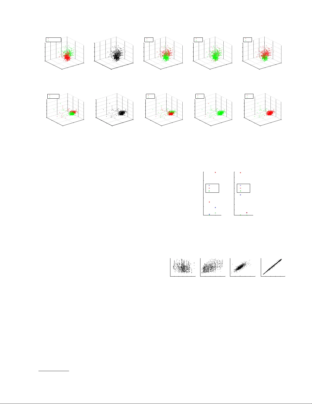
Iden tifying Finite Mixtures of Nonparametric Pro duct Distributions and Causal Inference of Confounders Eleni Sgouritsa 1 , Dominik Janzing 1 , Jonas P eters 1 , 2 , Bernhard Sc h¨ olk opf 1 1 Max Planc k Institute for Intelligen t Systems, T ¨ ubingen, Germany 2 Departmen t of Mathematics, ETH, Zurich { sgouritsa, janzing, p eters, bs } @tuebingen.mpg.de Abstract W e propose a kernel metho d to iden tify finite mixtures of nonparametric product distribu- tions. It is based on a Hilb ert space embed- ding of the join t distribution. The rank of the constructed tensor is equal to the num- b er of mixture components. W e present an algorithm to recov er the comp onen ts by par- titioning the data p oints into clusters suc h that the v ariables are join tly conditionally in- dep enden t giv en the cluster. This method can b e used to identify finite confounders. 1 In tro duction Laten t v ariable models are widely used to mo del het- erogeneit y in p opulations. In the following (Sections 2-4), we assume that the observ ed v ariables are jointly conditionally indep enden t given the latent class. F or example, giv en a medical syndrome, differen t symp- toms migh t be conditionally indep enden t. W e con- sider d ≥ 2 con tinuous observ ed random v ariables X 1 , X 2 ,. . . , X d with domains {X j } 1 ≤ j ≤ d and assume that their join t probabilit y distribution P ( X 1 , . . . , X d ) has a density with resp ect to the Leb esgue measure. W e introduce a finite (i.e., that tak es on v alues from a finite set) random v ariable Z that represen ts the laten t class with v alues in { z (1) , . . . , z ( m ) } . Assum- ing X 1 , . . . , X d to b e join tly conditionally indep enden t giv en Z (denoted b y X 1 ⊥ ⊥ X 2 ⊥ ⊥ . . . ⊥ ⊥ X d | Z ) im- plies the following decomp osition into a finite mixture of pro duct distributions: P ( X 1 , . . . , X d ) = m X i =1 P ( z ( i ) ) d Y j =1 P ( X j | z ( i ) ) (1) where P ( z ( i ) ) = P ( Z = z ( i ) ) 6 = 0. By p ar ameter identifiability of model (1), w e refer to the question of when P ( X 1 , . . . , X d ) uniquely deter- mines the following parameters: (a) the num ber of mixture components m , and (b) the distribution of eac h comp onent P ( X 1 , . . . , X d | z ( i ) ) and the mixing w eights P ( z ( i ) ) up to p erm utations of z -v alues. In this pap er, we focus on determining (a) and (b), when mo del (1) is iden tifiable. This can b e further used to infer the existence of a hidden common cause (con- founder) of a set of observed v ariables and reconstruct this confounder. The remainder of the pap er is orga- nized as follows: in Section 2, a metho d is prop osed to determine (a), i.e., the num b er of mixture comp onen ts m , Section 3 discusses established results on the identi- fiabilit y of the parameters in (b). Section 4 presen ts an algorithm for determining these parameters and Sec- tion 5 uses the findings of the previous sections for confounder iden tification. Finally , the exp erimen ts are pro vided in Section 6. 2 Iden tifying the Num b er of Mixture Comp onen ts V arious methods hav e b een prop osed in the litera- ture to select the num b er of mixture comp onents in a mixture mo del (e.g., F eng & McCullo c h (1996); B¨ ohning & Seidel (2003); Rasm ussen (2000); Iwata et al. (2013)). How ever, they imp ose different kind of assumptions than the conditional indep endence as- sumption of model (1) (e.g., that the distributions of the comp onen ts b elong to a certain parametric family). Assuming mo del (1), Kasahara & Shimotsu (2010) prop osed a nonparametric metho d that requires dis- cretization of the observed v ariables and provides only a low er b ound on m . In the follo wing, w e present a metho d to determine m in (1) without making para- metric assumptions on the comp onen t distributions. 2.1 Hilb ert Space Em b edding of Distributions Our metho d relies on representing P ( X 1 , . . . , X d ) as a v ector in a repro ducing kernel Hilb ert space (RKHS). W e briefly introduce this framework. F or a random v ariable X with domain X , an RKHS H on X with k ernel k is a space of functions f : X → R with dot pro duct h· , ·i , satisfying the repro ducing prop ert y (Sc h¨ olkopf & Smola, 2002): h f ( · ) , k ( x, · ) i = f ( x ), and consequen tly , h k ( x, · ) , k ( x 0 , · ) i = k ( x, x 0 ). The kernel th us defines a map x 7→ φ ( x ) := k ( x, . ) ∈ H satisfying k ( x, x 0 ) = h φ ( x ) , φ ( x 0 ) i , i.e., it corresp onds to a dot pro duct in H . Let P denote the set of probability distributions on X , then we use the following me an map (Smola et al., 2007) to define a Hilb ert space embedding of P : µ : P → H ; P ( X ) 7→ E X [ φ ( X )] (2) W e will henceforth assume this mapping to b e injec- tiv e, whic h is the case if k is char acteristic (F ukumizu et al., 2008), as the widely used Gaussian RBF kernel k ( x, x 0 ) = exp( − k x − x 0 k 2 / (2 σ 2 )). W e use the ab o ve framework to define Hilb ert space em b eddings of distributions of ev ery single X j . T o this end, we define k ernels k j for eac h X j , with feature maps x j 7→ φ j ( x j ) = k ( x j , . ) ∈ H j . W e thus obtain an em b edding µ j of the set P j in to H j as in (2). W e can apply the same framework to em b ed the set of join t distributions P 1 ,...,d on X 1 × . . . × X d . W e simply define a joint k ernel k 1 ,...,d b y k 1 ,...,d (( x 1 , . . . , x d ) , ( x 0 1 , . . . , x 0 d )) = Q d j =1 k j ( x j , x 0 j ), leading to a feature map in to H 1 ,...,d := N d j =1 H j with φ 1 ,...,d ( x 1 , . . . , x d ) = N d j =1 φ j ( x j ) (where N stands for the tensor pro duct). W e use the following mapping of the join t distribution: µ 1 ,...,d : P 1 ,...,d → d O j =1 H j (3) P ( X 1 , . . . , X d ) 7→ E X 1 ,...,X d [ d O j =1 φ j ( X j )] 2.2 Iden tifying the Number of Comp onen ts from the Rank of the Join t Embedding By linearit y of the maps µ 1 ,...,d and µ j , the embedding of the join t distribution decomp oses in to U X 1 ,...,X d := µ 1 ,...,d ( P ( X 1 , . . . , X d )) = m X i =1 P ( z ( i ) ) d O j =1 E X j [ φ j ( X j ) | z ( i ) ] . (4) Definition 1 (full rank conditional) L et A, B two r andom variables with domains A , B , r esp e ctively. The c onditional pr ob ability distribution P ( A | B ) is c al le d a ful l r ank c onditional if { P ( A | b ) } b with b ∈ B is a lin- e arly indep endent set of distributions. Recalling that the rank of a tensor is the minim um n umber of rank 1 tensors needed to express it as a linear com bination of them, we obtain: Theorem 1 (n umber of mixture comp onen ts) If P ( X 1 , . . . , X d ) is de c omp osable as in (1) and P ( X j | Z ) is a ful l r ank c onditional for al l 1 ≤ j ≤ d , then the tensor r ank of U X 1 ,...,X d is m . Pro of. F rom (4), the tensor rank of U X 1 ,...,X d is at most m . If the rank is m 0 < m , there exists another decomp osition of U X 1 ,...,X d (apart from (4)) as P m 0 i =1 N d j =1 v i,j , with non-zero v ec- tors v i,j ∈ H j . Then, there exists a v ector w ∈ H 1 , s.t. w ⊥ span { v 1 , 1 , . . . , v m 0 , 1 } and w 6 ⊥ span { ( E X 1 [ φ 1 ( X 1 ) | z ( i ) ]) 1 ≤ i ≤ m } . The dual vector , w i defines a linear form H 1 → R . By ov erloading notation, we consider it at the same time as a linear map H 1 ⊗ · · · ⊗ H d → H 2 ⊗ · · · ⊗ H d , b y extend- ing it with the identit y map on H 2 ⊗ · · · ⊗ H d . Then, h P m 0 i =1 N d j =1 v i,j , w i = P m 0 i =1 h v i 1 , w i N d j =2 v i,j = 0 but hU X 1 ,...,X d , w i 6 = 0. So, m = m 0 .  The assumption that P ( X j | Z ) is a full rank condi- tional, i.e., that { P ( X j | z ( i ) ) } i ≤ m is a linearly inde- p enden t set, is also used b y Allman et al. (2009) (see Sec. 3). It do es not preven t P ( X j | z ( q ) ) from b eing it- self a mixture distribution, how ever, it implies that, for all j, q , P ( X j | z ( q ) ) is not a linear combination of { P ( X j | z ( r ) ) } r 6 = q . Theorem 1 states that, under this assumption, the n umber of mixture comp onents m of (1) (or equiv alen tly the num ber of v alues of Z ) is iden- tifiable and equal to the rank of U X 1 ,...,X d . A straight- forw ard extension of Theorem 1 reads: Lemma 1 (infinite Z) If Z takes values fr om an in- finite set, then the tensor r ank of U X 1 ,...,X d is infinite. 2.3 Empirical Estimation of the T ensor Rank from Finite Data Giv en empirical data for every X j , { x (1) j , x (2) j , . . . , x ( n ) j } , to estimate the rank of (4), w e replace it with the empirical av erage ˆ U X 1 ,...,X d := 1 n n X i =1 d O j =1 φ j ( x ( i ) j ) , (5) whic h is known to con verge to the exp ectation in Hilb ert space norm (Smola et al., 2007). The v ector (5) still liv es in the infinite dimensional feature space H 1 ,...,d , which is a space of functions X 1 × · · · × X d → R . T o obtain a vector in a finite dimensional space, w e ev aluate this function at the n d data p oin ts ( x ( q 1 ) 1 , . . . , x ( q d ) d ) with q j ∈ { 1 , . . . , n } (the d -tuple of sup erscripts ( q 1 , . . . , q d ) runs ov er all elemen ts of { 1 , . . . , n } d ). Due to the repro ducing ker- nel prop ert y , this is equiv alen t to computing the inner pro duct with the images of these p oin ts under φ 1 ,...,d : V q 1 ,...,q d := * ˆ U X 1 ,...,X d , d O j =1 φ j ( x ( q j ) j ) + = 1 n n X i =1 d Y j =1 k j ( x ( i ) j , x ( q j ) j ) (6) F or d = 2, V is a matrix, so one can easily find low rank appro ximations via truncated Singular V alue Decom- p osition (SVD) by dropping low SVs. F or d > 2, find- ing a low-rank approximation of a tensor is an ill-p osed problem (De Silv a & Lim, 2008). By grouping the v ari- ables in to t wo sets, sa y X 1 , . . . , X s and X s +1 , . . . , X d without loss of generality , we can formally obtain the d = 2 case with t wo v ector-v alued v ariables. This amoun ts to reducing V in (6) to an n × n matrix by setting q 1 = · · · = q s and q s +1 = · · · = q d . In the- ory , we exp ect the rank to b e the same for all p ossible groupings. In practice, we rep ort the rank estimation of the ma jority of all groupings. The computational complexit y of this step is O (2 d − 1 N 3 ). 3 Iden tifiabilit y of Comp onen t Distributions and Mixing W eigh ts Once w e hav e determined the num b er of mixture com- p onen ts m , w e pro ceed to step (b) of recov ering the distribution of eac h comp onen t P ( X 1 , . . . , X d | z ( i ) ) and the mixing weigh ts P ( z ( i ) ). In the following, we de- scrib e results from the literature on when these pa- rameters are iden tifiable, for kno wn m . Hall & Zhou (2003) pro v ed that when m = 2, identifiabilit y of pa- rameters alwa ys holds in d ≥ 3 dimensions. F or d = 2 and m = 2 the parameters are generally not identi- fiable (there is a t wo-parameter con tinuum of solu- tions). In this case, one can obtain iden tifiability if, for all j , P ( X j | Z ) is pure (a conditional P ( X | Y ) is called pure if for an y tw o v alues y , y 0 of Y , the sum P ( X | y ) λ + P ( X | y 0 )(1 − λ ) is a probability distribu- tion only for λ ∈ [0 , 1] (Janzing et al., 2011)). Allman et al. (2009) established identifiabilit y of the param- eters whenever d ≥ 3 and for all m under weak con- ditions 1 , using a theorem of Krusk al (1977). Finally , Kasahara & Shimotsu (2010) provided complemen tary iden tifiability results for d ≥ 3 under differen t condi- tions with a constructiv e pro of. 1 the same assumption used in Theorem 1 that P ( X j | Z ) is a full rank conditional for all j . 4 Iden tifying Comp onen t Distributions and Mixing W eigh ts W e are given n data p oints from an iden tifiable dis- tribution P ( X 1 , . . . , X d ). Our goal is to cluster the data p oin ts (using m lab els) in suc h a w ay that the distribution of p oin ts with label i is close to the (un- observ ed) empirical distribution of ev ery mixture com- p onen t, P n ( X 1 , . . . , X d | z ( i ) ). 4.1 Existing Metho ds Probabilistic mixture mo dels or other clustering meth- o ds can be used to iden tify the mixture components (clusters) (e.g., V on Luxburg (2007); B¨ ohning & Seidel (2003); Rasmussen (2000); Iw ata et al. (2013)). How- ev er, they imp ose differen t kind of assumptions than the conditional indep endence assumption of mo del (1) (e.g., Gaussian mixture model). Assuming mo del (1), Levine et al. (2011) proposed an Exp ectation- Maximization (EM) algorithm for nonparametric es- timation of the parameters in (1), given that m is kno wn. Their algorithm uses a k ernel as smoothing op erator. They choose a common kernel bandwidth for all the comp onen ts b ecause otherwise their itera- tiv e algorithm is not guaran teed not to increase from one iteration to another. As stated also by Chauv eau et al. (2010), the fact that they do not use an adaptive bandwidth (Benaglia et al., 2011) can b e problematic esp ecially when the distributions of the comp onen ts differ significan tly . 4.2 Prop osed Method: Clustering with Indep endence Criterion (CLIC) The prop osed method, CLIC, assigns each of the n observ ations to one of the m (as estimated in Section 2) mixture comp onen ts (clusters). W e do not claim that eac h single data p oin t is assigned correctly (esp ecially when the clusters are o verlapping). Instead, w e aim to yield the v ariables join tly conditionally indep enden t giv en the cluster in order to recov er the comp onen ts. T o measure conditional independence of X 1 , . . . , X d giv en the cluster w e use the Hilb ert Sc hmidt Inde- p endence Criterion (HSIC) (Gretton et al., 2008). It measures the Hilb ert space distance betw een the ker- nel embeddings of the joint distribution of tw o (p os- sibly m ultiv ariate) random v ariables and the pro duct of their marginal distributions. If d > 2, we test for m utual indep endence. F or that, we perform multi- ple tests, namely: X 1 against ( X 2 , . . . , X d ), then X 2 against ( X 3 , . . . , X d ) etc. and use Bonferroni correc- tion. F or each cluster, w e consider as test statistic the HSIC from the test that leads to the smallest p -v alue (“highest” dep endence). W e regard the negative sum of the logarithms of all p - v alues (eac h one corresp onding to one cluster) under the null hypothesis of independence as our ob jective function. The proposed algorithm is iterativ e. W e first randomly assign ev ery data p oin t to one mixture comp onen t. In ev ery iteration we perform a greedy searc h: we randomly divide the data into disjoint sets of c points. Then, we select one of these sets and consider all p ossible assignments of the set’s p oin ts to the m clusters ( m c p ossible assignments). The assign- men t that optimizes the ob jective function is accepted and the p oin ts of the set are assigned to their new clusters (whic h may coincide with the old ones). W e, ev entually , rep eat the same pro cedure for all disjoint sets and this constitutes one ite ration of our algorithm. After ev ery iteration w e test for conditional indepen- dence given the cluster. The algorithm stops after an iteration when any of the following happ ens: we ob- serv e indep endence in all clusters, no data p oint has c hanged cluster assignment, an upp er limit of itera- tions is reached. It is clear that the ob jective function is monotonously decreasing. The algorithm may not succeed at pro ducing condi- tionally indep enden t v ariables for different reasons: e.g., incorrect estimation of m from the previous step or con v ergence to a local optim um. In that case, CLIC rep orts that it w as unable to find appropriate clusters. Along the iterations, the k ernel test of indep endence up dates the bandwidth according to the data points b elonging to the current cluster (in every dimension). Note, how ever, that this is not the case for the algo- rithm in Section 2. There, we are obliged to use a common bandwidth, because we do not hav e y et an y information ab out the mixture comp onen ts. The parameter c allo ws for a trade-off b et ween sp eed and a voiding local optima: for c = n , CLIC would find the global optimum after one step, but this would re- quire c hecking m n cluster assignmen ts. On the other hand, c = 1 leads to a faster algorithm that may get stuc k in lo cal optima. In all exp eriments we used c = 1 since we did not encounter man y problems with local optima. Considering c to b e a constant, the computa- tional complexity of CLIC is O ( m c N 3 ) for ev ery iter- ation. Algorithm 1 includes the pseudo co de of CLIC. 5 Causalit y: Iden tifying Confounders Dra wing causal conclusions from observ ed statistical dep endences without b eing able to interv ene on the system alwa ys relies on assumptions that link statis- tics to causality (Spirtes et al., 2001; P earl, 2000). The least disputed one is the Causal Marko v Condi- tion (CMC) stating that every v ariable is condition- ally independent of its non-descendant, giv en its par- Algorithm 1 CLIC 1: input data matrix X of size n × d , m , c 2: random assignmen t cluster ( i ) ∈ { 1 , . . . , m } , i = 1 , . . . , n of the data in to m clusters 3: while conditional dep endence giv en cluster and clusters c hange do 4: obj = computeO bj ( cluster ) 5: c ho ose random partition S j , j = 1 , . . . , J of the data in to sets of size c 6: for j = 1 to J do 7: new C l uster = cl uster 8: for all words w ∈ { 1 , . . . , m } c do 9: new C l uster ( S j ) = w 10: obj N ew ( w ) = computeObj ( new C l uster ) 11: end for 12: w Opt = argmin( obj N ew ) 13: cluster ( S j ) = w Opt 14: end for 15: end while 16: if conditional indep endence given cluster then 17: output cl uster 18: else 19: output “Unable to find appropriate clusters.” 20: end if en ts (Spirtes et al., 2001; Pearl, 2000) with resp ect to a directed acyclic graph (D AG) that formalizes the causal relations. W e fo cus on causal inference prob- lems where the set of observed v ariables ma y not be causally sufficien t, i.e. statistical dep endences can also b e due hidden common causes (confounders) of tw o or more observed v ariables. Under the assumption of lin- ear relationships betw een v ariables and non-Gaussian distributions, confounders ma y b e iden tified using In- dep enden t Component Analysis (Shimizu et al., 2009). Other results for the linear case are presented in Silv a et al. (2006) and for the non-linear case with addi- tiv e noise in Janzing et al. (2009). F ast Causal Infer- ence (Silv a et al., 2006) can exclude confounding for some pairs of v ariables, given that many v ariables are observ ed. Finally , the reconstruction of binary con- founders under the assumption of pure conditionals is presen ted in Janzing et al. (2011). In this section, w e use the results of the previous sec- tions to infer the existence and iden tify a finite con- founder that explains all the dep endences b et ween the observ ed v ariables. W e assume that laten t v ariables are not caused b y observed v ariables (the same as- sumption has b een used by Silv a et al. (2006)). Unlik e previous metho ds, we do not make explicit assump- tions on the distribution of the v ariables. Instead, w e p ostulate a differen t assumption, namely that the con- ditional of eac h v ariable given its parents is full rank: Assumption 1 (full rank giv en parents) L et P A Y denote the p ar ents of a c ontinuous variable Y with r esp e ct to the true c ausal DA G. Then, P ( Y | P A Y ) is a ful l r ank (f.r.) c onditional. Lemma 2 (full rank giv en parent) By Assump- tion 1 it fol lows that, if A ∈ P A Y is one of the p ar ents of Y , i.e., A → Y , then, sinc e P ( Y | P A Y ) is a f.r. c onditional, P ( Y | A ) is also a f.r. c onditional (after mar ginalization). Remark: If Assumption 1 holds and A → B → C , then P ( B | A ) and P ( C | B ) are f.r. conditionals (Lemma 2), whic h implies that P ( C | A ) is also a f.r. conditional, since it results from their m ultiplication. Lemma 3 (shifted copies) L et R b e a pr ob ability distribution on R and T t R its c opy shifte d by t ∈ R to the right. Then { T t R } t ∈ R ar e line arly indep endent. Pro of. Let q X j =1 α j T t j R = 0 , (7) for some q and some q -tuple α 1 , . . . , α q . Let ˆ R b e the F ourier transform of R . I f we set g ( ω ) := P q j =1 α j e iω t j then (7) implies g ( ω ) ˆ R ( ω ) = 0 for all ω ∈ R , hence g v anishes for all ω with ˆ R ( ω ) 6 = 0, whic h is a set of non-zero measure. Since g is holomorphic, it therefore v anishes for all ω ∈ R and th us all coefficients are zero.  The following theorem sho ws that Assumption 1 is typ- ically satisfied for a class of causal models considered b y Hoy er et al. (2009): Theorem 2 (additiv e noise mo del) L et Y b e given by Y = f ( P A Y ) + N , wher e N is a noise variable that is statistic al ly indep endent of P A Y and f is an inje ctive function. Then P ( Y | P A Y ) is a ful l r ank c onditional. The proof is a straigh tforw ard application of Lemma 3. Theorem 3 (rank of cause-effect pair) Assume ther e is a dir e ct c ausal link A → B b etwe en two observe d variables A and B , with { A , B } not ne c es- sarily b eing a c ausal ly sufficient set (i.e., ther e may b e unobserve d c ommon c auses of A and B ). Then, given Assumption 1, the r ank of U A,B is e qual to the numb er of values that A takes, if A is finite. If A is infinite, then the r ank of U A,B is infinite. Pro of. By Assumption 1, P ( B | A ) is a f.r. conditional (Lemma 2). Since A ⊥ ⊥ B | A , applying Theorem 1 for finite Z := A we conclude that the rank of U A,B is equal to the num b er of v alues of A . F or infinite A , we similarly apply Lemma 1 and we get infinite rank of U A,B .  Theorem 4 (rank of confounded pair) Assume A ← C → B , and A , B do not have other c ommon c auses ap art fr om C . Then, given Assumption 1, the r ank of U A,B is e qual to the numb er of values of C . Pro of. The pro of is straigh tforw ard: by Assump- tion 1, P ( A | C ) and P ( B | C ) are f.r. conditionals (Lemma 2). Additionally , A ⊥ ⊥ B | C and then, ac- cording to Theorem 1, the rank of U A,B is equal to the n umber of v alues of Z := C (for infinite C , the rank is infinite).  Theorems 3 and 4 state what is the expected rank of U A,B for v arious causal structure scenarios. How ever, in causal inference we are in terested in inferring the unknown underlying causal DA G. The following Theo- rem uses Theorem 3 to infer the causal structure based on the rank of the embedding of the join t distribution. Theorem 5 (iden tifying confounders) L et Y 1 , . . . , Y d denote al l observe d variables. Assume they ar e c ontinuous, p airwise dep endent, and ther e is at most one (if any) hidden c ommon c ause of two or mor e of the observe d variables. If Assumption 1 holds and the r ank of U Y 1 ,...,Y d , with d ≥ 3 , is finite, then Fig. 1 depicts the only p ossible c ausal DA G with W b eing an unobserve d variable and P ( Y 1 , . . . , Y d , W ) is identifiable up to r ep ar ameterizations of W . Pro of. Assume there is at least one direct causal link Y i → Y i 0 . Then, according to Theorem 3, the rank of U Y i ,Y i 0 , and th us the rank of U Y 1 ,...,Y d , would b e infinite. Therefore, direct causal links b et ween the { Y j } can b e excluded and the statistical depen- dencies betw een { Y j } can only b e explained by hid- den common causes. Since w e assumed that there is at most one hidden common cause (and the ob- serv ed v ariables are pairwise dep endent), the only p os- sible causal graph is depicted in Fig. 1. This implies Y 1 ⊥ ⊥ Y 2 ⊥ ⊥ . . . ⊥ ⊥ Y d | W (according to the CMC), so mo del (1) holds, with Z := W being the latent v ari- able. According to the previous sections (Theorem 1 and Section 3), this mo del is identifiable.  Based on Theorem 1, the num b er of v alues of W is equal to the rank of U Y 1 ,...,Y d and P ( Y 1 , . . . , Y d , W ) can b e iden tified according to Section 4. Note that the single common cause W could b e the result of merging man y common causes W 1 , .., W k to one v ector-v alued v ariable W . Thus, at first glance, it seems that one do es not lose generalit y b y assuming only one common cause. Ho wev er, Assumption 1, then, excludes the case where W consists of components each of whic h only acts on some different subset of the { Y j } . W 1 , .., W k should all b e common causes of all { Y j } . W Y 1 Y 2 Y d Figure 1: Inferred causal DA G (the dotted circle rep- resen ts an unobserved v ariable). Note that, when w e are giv en only finite data, the esti- mated rank of U Y 1 ,...,Y d is alw ays finite, highly depend- ing on the strength of the causal arro ws and the sample size. Then, we are faced with the issue that, based on Theorem 5, w e would alwa ys infer that Fig. 1 depicts the only p ossible causal DA G, with the num b er of v al- ues of W being equal to the estimated rank. Ho wev er, the lo w er the rank, the more confiden t w e get that this is, indeed, due to the existence of a confounder that renders the observed v ariables conditionally inde- p enden t (Fig. 1). On the other hand, high rank can also be due to direct causal links b et ween the observ ed v ariables or con tin uous confounders. F or that, we con- sider Theorem 5 to b e more appropriate for inferring the existence of a confounder with a small n umber of v alues which would lead to low rank. Ho wev er, w e ad- mit that what is considered “high” or “lo w” is not w ell defined. F or example, ho w muc h “high” rank v alues w e exp ect for the D AG Y 1 → Y 2 highly dep ends on the strength of the causal arrow: the low er the dep en- dence betw een Y 1 and Y 2 is, the low er is, generally , the estimated rank. In practice, w e could make a v ague suggestion that whenev er the estimated rank is b elo w 5 (although the dep endence betw een { Y j } is strong), it is quite probable that this is due to a confounder (Fig. 1) but for higher rank it is getting more difficult to decide on the underlying causal structure. 6 Exp erimen ts W e conducted experiments both on sim ulated and real data. In all our exp erimen ts w e use a Gaussian RBF k ernel k ( x, x 0 ) = exp  −k x − x 0 k 2 / (2 σ 2 )  . Concerning the first step of determining the num b er of mixture comp onen ts: a common w ay to select the bandwidth σ j for every k j is to set it to the median distance b e- t ween all data points in the j th dimension of the em- pirical data. How ev er, this approach would usually result in an ov erestimation of the bandwidth, espe- cially in case of many mixture components (see also Benaglia et al. (2011)). T o partially account for this, w e compute the bandwidth for every X j as the median distance b et ween p oin ts in the neighborho od of every p oin t in the sample. The neigh b orho od is found b y the 10 nearest neighbors of each p oin t computed using all other v ariables apart from X j . T o estimate the rank of V , w e find its SVD and report the estimated rank as ˆ m = argmin i ( S V i +1 /S V i ) within the SVs that co v er 90-99.999% of the total v ariance. Finally , concerning CLIC, we use 7 as the maxim um num ber of iterations, but usually the algorithm terminated earlier. 6.1 Sim ulated Data Sim ulated data were generated according to the DA G of Fig. 1 (w e henceforth refer to them as the first set of sim ulated data), e.i., mo del (1) holds with Z := W , since Y 1 ⊥ ⊥ Y 2 ⊥ ⊥ . . . ⊥ ⊥ Y d | W . W e first generated Z from a uniform distribution on m v alues. Then, the distribution of eac h mixture comp onen t in ev ery di- mension ( P ( X j | z ( i ) )) was chosen randomly b et ween: (i) a normal distribution with standard deviation 0.7, 1, or 1.3, (ii) a t-distribution with degrees of freedom 3 or 10, (iii) a (stretched) b eta distribution with alpha 0.5 or 1 and b eta 0.5 or 1, and (iv) a mixture of tw o normal distributions with v ariance 0.7 for eac h. The distance b et w een the comp onen ts in each dimension w as distributed according to a Gaussian with mean 2 and standard deviation 0.3. W e chose the distance and the mixtures such that the exp erimen ts cov er dif- feren t levels of o verlap betw een the comp onen ts, and at the same time { P ( X j | z ( i ) ) } i ≤ m are generically lin- early indep enden t. W e ran 100 exp erimen ts for each com bination of d = 2 , 3 , 5 and m = 2 , 3 , 4 , 5, with the sample size b eing 300 × m . F or comparison, w e additionally generated data where the observed v ariables are connected also with di- rect causal links and thus are conditionally dep enden t giv en the confounder (we henceforth refer to them as the second set of sim ulated data). F or that, we first generated data according to the D AG of Fig. 1, as ab o v e, for d = 2 and m = 1 (whic h amounts to no confounder) and for d = 2 and m = 3 (3-state con- founder). X 2 w as then shifted by 4 X 1 to sim ulate a di- rect causal link X 1 → X 2 . In this case, X 1 ⊥ ⊥ X 2 | X 1 , so w e hav e infinite Z := X 1 . 6.1.1 Iden tifying the Number of Mixture Comp onen ts 1 2 3 4 5 6 7 8 9 10 0 20 40 60 80 Estimated m 1 2 3 4 5 6 7 8 9 10 0 20 40 60 80 100 Estimated m 1 2 3 4 5 6 7 8 9 10 0 20 40 60 80 100 Estimated m Figure 2: Histograms of the estimated num b er of mix- ture comp onen ts m for the first set of simulated data, for m = 2 throughout, and d = 2 (left), d = 3 (mid- dle), d = 5 (righ t). W e first rep ort results on the first part of identifica- 1 2 3 4 5 6 7 8 9 10 0 20 40 60 80 Estimated m 1 2 3 4 5 6 7 8 9 10 0 20 40 60 80 100 Estimated m 1 2 3 4 5 6 7 8 9 10 0 20 40 60 80 100 Estimated m Figure 3: As Figure 2 but for m = 3. 1 2 3 4 5 6 7 8 9 10 0 20 40 60 Estimated m 1 2 3 4 5 6 7 8 9 10 0 20 40 60 80 100 Estimated m 1 2 3 4 5 6 7 8 9 10 0 20 40 60 80 100 Estimated m Figure 4: As Figure 2 but for m = 4. 1 2 3 4 5 6 7 8 9 10 0 20 40 60 Estimated m 1 2 3 4 5 6 7 8 9 10 0 20 40 60 80 Estimated m 1 2 3 4 5 6 7 8 9 10 0 20 40 60 80 100 Estimated m Figure 5: As Figure 2 but for m = 5. tion, i.e. identifying the num b er of mixture comp o- nen ts m in (1). The empirical rank estimation may dep end on the strength of the causal arro ws, the ker- nel bandwidth selection, the sample size and the wa y to estimate the rank b y k eeping only large eigen v alues. Figures 2, 3, 4 and 5 illustrate histograms of the es- timated n umber of comp onen ts (equiv alen tly the esti- mated n um b er of v alues of the confounder) for the first set of simulated data for m = 2 , 3 , 4 and 5, respectively . Eac h figure contains one histogram for every v alue of d = 2 , 3 and 5. W e can observe that as m increases the metho d b ecomes more sensitive in underestimat- ing the num b er of components, a b eha vior whic h can b e explained b y the common sigma selection for all the data in eac h dimension or by high ov erlap of the distri- butions (which could violate Assumption 1). On the other hand, as d increases the metho d b ecomes more robust in estimating m correctly due to the group- ing of v ariables that allows m ultiple rank estimations. The “lo w” estimated rank v alues pro vide us with some evidence that the causal DA G of Fig. 1 is true (Theo- rem 5). Of course, as stated also at the end of Sec. 5, it is difficult to define what is considered a low rank. Figure 6 depicts histograms of the estimated num ber of components for the second set of simulated data. According to Theorem 3, the direct causal link X 1 → X 2 results in an infinite rank of U X 1 ,X 2 . Indeed, we can observe that in this case the estimated m is muc h higher. The “high” estimated rank v alues provide us with some evidence that the underlying causal D AG ma y include direct causal links betw een the observ ed v ariables or confounders with a high or infinite n umber of v alues. Note that, dep ending on the strength of the causal arrow X 1 → X 2 , w e ma y get higher or low er rank v alues. F or example, if the strength is very weak w e get lo w er rank v alues since the dep endence betw een X 1 and X 2 tends to be dominated by the confounder (that has a small n umber of v alues). 0 5 10 15 20 25 30 35 40 45 0 5 10 15 20 Estimated m 0 5 10 15 20 25 30 35 40 45 0 5 10 15 Estimated m Figure 6: Histograms of the estimated m for the second set of sim ulated data (including a direct causal arro w). Left: no confounder, right: 3-state confounder. 6.1.2 F ull Identification F ramework Next, we performed experiments, using the first set of simulated data to ev aluate the p erformance of the prop osed metho d (CLIC) (Section 4.2), the metho d of Levine et al. (2011) (Section 4.1) and the EM algo- rithm using a Gaussian mixture mo del (EM is rep eated 5 times and the solution with the largest lik elihoo d is rep orted). In the following, we refer to these meth- o ds as CLIC, Levine, and EM, resp ectiv ely . F or eac h data point, the tw o latter metho ds output p osterior probabilities for the m clusters, which w e sample from to obtain cluster assignments. Figure 7 illustrates the cluster assignments of these three metho ds for one sim- ulated dataset with m = 3 and d = 2 (this is more for visualization purp oses b ecause for these v alues of d and m mo del (1) is not alwa ys identifiable). Note that p erm utations of the colors are due to the ambi- guit y of lab els in the identification problem. How ev er, EM incorrectly identifies a single comp onen t (having a mixture of tw o Gaussians as marginal density in X 1 dimension) as tw o distinct comp onents. It is clear that this is b ecause it assumes that the data are generated b y a Gaussian mixture model and not by mo del (1), as opp osed to CLIC and Levine metho ds. W e compare the distribution of eac h cluster output (for each of the three metho ds) to the empirical distri- bution, P n ( X 1 , . . . , X d | z ( i ) ), of the corresponding mix- ture comp onen t (ground truth). F or that w e use the squared maxim um mean discrepancy (MMD) (Gret- ton et al., 2012) that is the distance b et w een Hilb ert space em b eddings of distributions. W e only use the MMD and not one of the test statistics describ ed in Gretton et al. (2012), since they are designed to com- pare t wo indep endent samples, whereas our samples −4 −2 0 2 4 6 8 −4 −2 0 2 4 6 8 X1 X2 Z = 1 Z = 2 Z = 3 −4 −2 0 2 4 6 8 −4 −2 0 2 4 6 8 X1 X2 −4 −2 0 2 4 6 8 −4 −2 0 2 4 6 8 X1 X2 Z = 1 Z = 2 Z = 3 −4 −2 0 2 4 6 8 −4 −2 0 2 4 6 8 X1 X2 Z = 1 Z = 2 Z = 3 −4 −2 0 2 4 6 8 −4 −2 0 2 4 6 8 X1 X2 Z = 1 Z = 2 Z = 3 Figure 7: F rom left to righ t: ground truth, input, CLIC output, Levine output, and EM output for simulated data generated for m = 3. Eac h color represents one mixture comp onen t. 0 50 100 150 200 −0.05 0 0.05 0.1 0.15 0.2 0.25 0.3 0.35 0.4 0.45 cluster index squared mmd EM Levine CLIC (a) 0 50 100 150 200 250 300 −0.2 0 0.2 0.4 0.6 0.8 1 1.2 cluster index squared mmd EM Levine CLIC (b) 0 50 100 150 200 −0.02 0 0.02 0.04 0.06 0.08 0.1 0.12 0.14 0.16 cluster index squared mmd EM Levine CLIC (c) Figure 8: Squared MMD betw een output and ground truth clusters (for eac h of the three methods) for sim ulated data with (a) d = 3 , m = 2, (b) d = 3 , m = 3 and (c) d = 5 , m = 2 (output and ground truth) ha ve ov erlapping observ a- tions. T o account for the permutations, we measure the MMD for all cluster p erm utations and select the one with the minimum sum of MMD for all clusters. Figures 8(a)-8(c) rep ort the squared MMD results of the three metho ds for differen t combinations of m and d . Each p oint corresp onds to the squared MMD for one cluster of one of the 100 exp erimen ts. Results are pro vided only for the cases that the num ber of com- p onen ts m was correctly iden tified from the previous step. The CLIC metho d was unable to find appropri- ate clusters in 2 exp eriments for d = 3 and m = 3 and in 13 for d = 5 and m = 2. Without claiming that the comparison is exhaustive, w e can infer that both CLIC and Levine metho ds p erform significantly b etter than EM, since they imp ose conditional indep endence. F or higher d , EM improv es since the clusters are less ov er- lapping. How ev er, the computational time of CLIC is higher compared to the other t wo metho ds. 6.2 Real data F urther, we applied our framework to the Breast Cancer Wisconsin (Diagnostic) Data Set from the UCI Machine Learning Rep ository (F rank & Asun- cion, 2010). The dataset consists of 32 features of breast masses along with their classification as b e- nign (B) or malignant (M). The sample size of the dataset is 569 (357 (B), 212 (M)). W e selected 3 fea- 40 60 80 100 120 140 160 180 200 0 500 1000 1500 2000 2500 3000 perimeter area BENIGN MALIGNANT 40 60 80 100 120 140 160 180 200 0 0.05 0.1 0.15 0.2 0.25 0.3 0.35 0.4 0.45 perimeter concavity BENIGN MALIGNANT Figure 10: Breast data: features conditionally depen- den t given the class. Left: estimated m = 62, right: estimated m = 8. tures, namely p erimeter, compactness and texture, whic h are pairwise dependent (the minim um p-v alue is pv al = 2 . 43 e − 17), but b ecome (close to) mutu- ally indep enden t when w e condition on the class (B or M) ( pv al B = 0 . 016 , pv al M = 0 . 013). W e applied our metho d to these three features (assuming the class is unkno wn) and w e succeeded at correctly inferring that the num b er of mixture components is 2. Figure 9 de- picts the ground truth of the breast data, the input and the results of CLIC, Levine and EM, and Fig. 12(a) the corresp onding squared MMDs. W e can observe that Levine metho d p erforms v ery p oorly for this datase t. Additionally , we selected differen t features, namely p erimeter and area, and conca vity and area, whic h are not conditionally indep enden t given the binary class. 0 50 100 150 200 0 0.2 0.4 0 10 20 30 40 perimeter compactness texture BENIGN MALIGNANT 0 50 100 150 200 0 0.2 0.4 0 10 20 30 40 perimeter compactness texture 0 50 100 150 200 0 0.2 0.4 0 10 20 30 40 perimeter compactness texture Z = 1 Z = 2 0 50 100 150 200 0 0.2 0.4 0 10 20 30 40 perimeter compactness texture Z = 1 Z = 2 0 50 100 150 200 0 0.2 0.4 0 10 20 30 40 perimeter compactness texture Z = 1 Z = 2 Figure 9: F rom left to right: ground truth, input, output CLIC, Levine, and EM for the breast data. 100 150 200 50 100 150 200 −200 −100 0 100 200 300 height QRS duration QRSTA of channel V1 MALE FEMALE 100 150 200 50 100 150 200 −200 −100 0 100 200 300 height QRS duration QRSTA of channel V1 100 150 200 50 100 150 200 −200 −100 0 100 200 300 height QRS duration QRSTA of channel V1 Z = 1 Z = 2 100 150 200 50 100 150 200 −200 −100 0 100 200 300 height QRS duration QRSTA of channel V1 Z = 1 Z = 2 100 150 200 50 100 150 200 −200 −100 0 100 200 300 height QRS duration QRSTA of channel V1 Z = 1 Z = 2 Figure 11: F rom left to right: ground truth, input, output CLIC, Levine, and EM for the arrhythmia data. In this case, w e got rank v alues higher than tw o, i.e., 62 and 8, resp ectiv ely (Fig. 10). W e similarly applied our framew ork to the Arrh ythmia Data Set (sample size 452) (F rank & Asuncion, 2010). W e selected 3 features, namely heigh t, QRS duration and QRST A of channel V1 whic h are dep enden t (min- im um pv al = 8 . 96 e − 05), but b ecome indep enden t when we condition on a fourth feature, the sex of a p erson (Male or F emale) ( pv al M = 0 . 0607 , pv al F = 0 . 0373). W e applied our metho d to the three fea- tures and w e succeeded at correctly inferring that the n umber of mixture components is 2. Figure 11 de- picts the ground truth, the input and the results of CLIC, Levine and EM, and Fig. 12(b) the corresp ond- ing squared MMDs. W e can observe that Levine and EM metho ds p erform very p oorly for this dataset. Finally , w e applied our method to a database with cause-effect pairs 2 . It includes pairs of v ariables with kno wn causal structure. Since there exists a direct causal arro w X → Y , we expect the rank of U X,Y to b e infinite given our assumptions (Theorem 3), ev en if there exist hidden confounders or not. How- ev er, the estimated rank from finite data is alwa ys fi- nite, its magnitude strongly dep ending on the strength of the causal arrow and the sample size, as men- tioned in Sec. 5. Figure 13 depicts 4 cause-effect pairs (which w ere tak en from the UCI Machine Learn- ing Rep ository (F rank & Asuncion, 2010)) with the same sample size (1000 data p oin ts) but v arious de- grees of dep endence, sp ecifically: pv al = 7 . 16 e − 12, pv al = 9 . 41 e − 63, pval = 1 . 21 e − 317, pv al = 0. The estimated ranks are m = 1 , 4 , 8 and 63, respectively . Note that when X and Y are close to indep enden t (e.g., the first plot of Fig. 13) the assumption of pair- 2 h ttp://webdav.tuebingen.mpg.de/cause-effect/ wise dep endence of Theorem 5 is almost violated. 1 2 0 0.05 0.1 0.15 0.2 0.25 cluster index squared mmd EM Levine CLIC (a) 1 2 0 0.1 0.2 0.3 0.4 0.5 0.6 0.7 0.8 cluster index squared mmd EM Levine CLIC (b) Figure 12: Squared MMD betw een output and ground truth clusters for (a) breast and (b) arrh ythmia data. −3 −2 −1 0 1 2 3 −3 −2 −1 0 1 2 3 X Y −2 −1 0 1 2 3 −3 −2 −1 0 1 2 3 X Y −4 −2 0 2 4 6 −5 0 5 X Y −3 −2 −1 0 1 2 −3 −2.5 −2 −1.5 −1 −0.5 0 0.5 1 1.5 X Y Figure 13: F our cause-effect pairs. Estimated m from left to righ t: m = 1, m = 4, m = 8, and m = 63. 7 Conclusion In this pap er, we introduced a kernel metho d to iden- tify finite mixtures of nonparametric pro duct distri- butions. The metho d was further used to infer the existence and identify a hidden common cause of a set of observ ed v ariables. Exp erimen ts on sim ulated and real data were p erformed for ev aluation of the pro- p osed approach. In practice, our metho d is more ap- propriate for the identification of a confounder with a small n umber of v alues. References Allman, E. S., Matias, C., and Rhodes, J. A. Identifia- bilit y of parameters in latent structure mo dels with man y observ ed v ariables. The Annals of Statistics , 37:3099–3132, 2009. Benaglia, M., Chauveau, D., and Hunter, D. R. Band- width selection in an EM-lik e algorithm for nonpara- metric multiv ariate mixtures. In Nonp ar ametrics and Mixtur e Mo dels , 2011. B¨ ohning, D. and Seidel, W. Editorial: recen t develop- men ts in mixture models. Computational Statistics & Data A nalysis , 41(3):349–357, 2003. Chauv eau, D., Hunter, D. R., and Levine, M. Estima- tion for conditional independence multiv ariate finite mixture mo dels. T e chnic al R ep ort , 2010. De Silv a, V. and Lim, L.H. T ensor rank and the ill- p osedness of the b est low-rank appro ximation prob- lem. SIAM Journal on Matrix Analysis and Appli- c ations , 30(3):1084–1127, 2008. F eng, Z. D. and McCullo c h, C. E. Using b ootstrap lik eliho o d ratios in finite mixture mo dels. Journal of the R oyal Statistic al So ciety. Series B (Metho d- olo gic al) , 58(3):609–617, 1996. F rank, A. and Asuncion, A. UCI machine learning rep ository , 2010. URL http://archive.ics.uci. edu/ml . F ukumizu, K., Gretton, A., Sun, X., and Sc h¨ olkopf, B. Kernel measures of conditional dependence. In A d- vanc es in Neur al Information Pr o c essing Systems , v olume 20, pp. 489–496. MIT Press, 09 2008. Gretton, A., F ukumizu, K., T eo, C. H., Song, L., Sc h¨ olkopf, B., and Smola, A. A kernel statistical test of independence. In A dvanc es in Neur al Infor- mation Pr o c essing Systems 20 , pp. 585–592, Cam- bridge, 2008. MIT Press. Gretton, A., Borgwardt, K., Rasch, M., Sch¨ olk opf, B., and Smola, A. A kernel tw o-sample test. Journal of Machine L e arning R ese ar ch , 13:671 –721, 2012. Hall, P . and Zhou, X.-H. Nonparametric estimation of comp onen t distributions in a m ultiv ariate mixture. The Annals of Statistics , 31(1):201–224, 2003. Ho yer, P ., Janzing, D., Mooij, J., Peters, J., and Sc h¨ olkopf, B. Nonlinear causal discov ery with addi- tiv e noise models. In A dvanc es in Neur al Informa- tion Pr o c essing Systems 2008 . MIT Press, 2009. Iw ata, T., Duv enaud, D., and Ghahramani, Z. W arp ed mixtures for nonparametric cluster shap es. In Un- c ertainty in A rtificial Intel ligenc e , 2013. Janzing, D., P eters, J., Mo oij, J., and Sc h¨ olkopf, B. Iden tifying latent confounders using additive noise mo dels. In Unc ertainty in Artificial Intel ligenc e , pp. 249–257, 2009. Janzing, D., Sgouritsa, E., Stegle, O., Peters, J., and Sc h¨ olkopf, B. Detecting low-complexit y unobserved causes. In Unc ertainty in Artificial Intel ligenc e , pp. 383–391, 2011. Kasahara, H. and Shimotsu, K. Nonparametric iden ti- fication of multiv ariate mixtures. T ec hnical report, 2010. Krusk al, J. B. Three-wa y arra ys: rank and unique- ness of trilinear decomp ositions, with application to arithmetic complexit y and statistics. Line ar Algebr a and its Applic ations , 18(2):95 – 138, 1977. Levine, M., Hunter, D. R., and Chauveau, D. Maxi- m um smo othed lik eliho od for m ultiv ariate mixtures. Biometrika , 98(2):403–416, 2011. P earl, J. Causality . Cambridge Univ ersit y Press, 2000. Rasm ussen, Carl Edward. The infinite gaussian mix- ture mo del. A dvanc es in Neur al Information Pr o- c essing Systems , 12(5.2):2, 2000. Sc h¨ olkopf, B. and Smola, A. L e arning with kernels . MIT Press, Cam bridge, MA, 2002. Shimizu, S., Ho yer, P ., and Hyv¨ arinen, A. Estima- tion of linear non-gaussian acyclic mo dels for latent factors. Neur o c omputing , 72(7–9):2024–2027, 2009. Silv a, R., Scheines, R., Glymour, C., and Spirtes, P . Learning the structure of linear laten t v ariable mo d- els. JMLR , 7:191–246, 2006. Smola, A., Gretton, A., Song, L., and Sch¨ olk opf, B. A hilb ert space embedding for distributions. In A lgorithmic L e arning The ory , pp. 13–31. Springer- V erlag, 2007. Spirtes, P ., Glymour, C., and Scheines, R. Causation, Pr e diction, and Se ar ch . MIT Press, 2. edition, 2001. V on Luxburg, U. A tutorial on sp ectral clustering. Statistics and c omputing , 17(4):395–416, 2007.