Cyclic Causal Discovery from Continuous Equilibrium Data

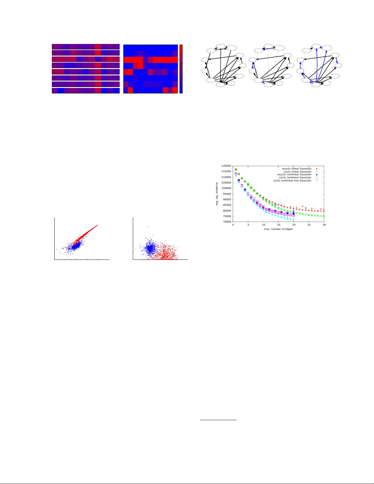
Cyclic Causal Disco v ery from Con tin uous Equilibrium Data Joris M. Mo oij ∗ Informatics Institute Univ ersity of Amsterdam The Netherlands T om Hesk es Institute for Computing and Information Sciences Radb oud Univ ersity Nijmegen The Netherlands Abstract W e prop ose a metho d for learning cyclic causal mo dels from a combination of obser- v ational and in terv entional equilibrium data. No vel asp ects of the prop osed metho d are its abilit y to w ork with con tinuous data (without assuming linearity) and to deal with feedback lo ops. Within the context of biochemical re- actions, we also prop ose a nov el wa y of mo d- eling in terven tions that modify the activity of comp ounds instead of their abundance. F or computational r easons, we approximate the nonlinear causal mechanisms by (coupled) lo- cal linearizations, one for eac h exp erimental condition. W e apply the method to recon- struct a cellular signaling netw ork from the flo w cytometry data measured b y Sachs et al. (2005). W e show that our metho d finds evi- dence in the data for feedback loops and that it gives a more accurate quan titative descrip- tion of the data at comparable mo del com- plexit y . 1 In tro duction A central question that arises in many empirical sci- ences is how to discov er cause- effect relationships b e- t ween v ariables from measured data. Kno wledge of causal relationships is essen tial in order to predict ho w a system will react to interv entions that p erturb the system from its natural state (Pearl, 2000), whic h is v ery useful for many practical applications. An exam- ple from biology is the problem of predicting in silic o ho w a signaling path wa y in a cell will react in vitr o when it is treated with a certain chemical comp ound. The abilit y to reliably mak e suc h causal predictions ∗ Also affiliated to Institute for Computing and Informa- tion Sciences, Radboud Universit y Nijmegen, The Nether- lands can b e a p ow erful tool for practical applications lik e drug design. A concrete example is the m ultiv ariate proteomics data set measured and analyzed b y Sac hs et al. (2005). Using flo w cytometry , abundances of 11 biochemi- cal c ompounds (phosphorylated proteins and phospho- lipid comp onen ts) w ere measured in single human im- m une system cells under v arious exp erimental p ertur- bations. Sachs et al. (2005) reconstructed the underly- ing “signaling net work” b y learning Ba y esian net works from the data. Their reconstruction turned out to be v ery close to the “well-established consensus netw ork” that had been obtained b y manually combining results from many different exp erimen ts, an effort that had tak en ab out tw o decades. The consensus netw ork contains 18 expected causal relationships. Sachs et al. (2005) found tw o new un- exp ected causal relations (and exp erimen tally verified one of them) and obtained one reversed relationship. Ho wev er, they did not reco ver three of the 18 expected causal relationships. Sac hs et al. (2005) h yp othesized that these three missing causal relationships are all in- v olved in feedback lo ops. As Ba yesian netw orks are acyclic by definition, this could explain why they were not found by their metho d. Additional supp ort for this hypothesis can b e found b y simple insp ection of the data, which already sho ws strong evidence for the presence of feedback lo ops. In later work (Itani et al., 2010), the authors prop osed a heuristic method for causal disco very that tak es in to account the possibility of feedbac k. An alternativ e approac h to dealing with cycles w as prop osed by Schmidt and Murphy (2009). A common feature of the causal disco very metho ds that hav e b een applied so far on this protein data set is that they all work with discr etize d data: although the ra w measuremen ts are con tinuous-v alued, the data is prepro cessed by discretization into three coarse cat- egories (lo w, medium and high abundance). W e argue that discretization of the data as a prepro cessing step should b e a voided if p ossible, as this thro ws a wa y muc h of the information in the data that could b e useful for causal disco very . Recen tly , several metho ds hav e b een prop osed for causal disco very from contin uous-v alued observ ational data by exploiting indep endence of the estimated noise with the input (Shimizu et al., 2006; Ho yer et al., 2009; Zhang and Hyv¨ arinen, 2009; Pe- ters et al., 2011). Similar ideas hav e also b een studied in the cyclic case (Lacerda et al., 2008; Mo oij et al., 2011). More recently , cyclic metho ds that can deal with hidden common causes and with a combination of observ ational and exp erimental data ha v e b een pro- p osed (Eb erhardt et al., 2010; Hyttinen et al., 2012). Ho wev er, none of these methods are directly applica- ble to the (Sachs et al., 2005) data set, among others b ecause they mo del interv entions in a different wa y . Most in terven tions p erformed by Sachs et al. (2005) c hange the activity of a comp ound, not its abundanc e , and therefore the standard formalism for in terven tions (P earl, 2000) is not applicable. Sac hs et al. (2005) and Itani et al. (2010) prop ose tw o different wa ys of mo deling these interv entions that both exploit the fact that the data has been discretized. Eaton and Murphy (2007) consider differen t possible in terven tion t yp es and learn the interv entions from the data, instead of using the biological background knowledge in (Sachs et al., 2005). Eaton and Murphy (2007) conclude that the data can b e b est explained by assuming that most in terven tions are not as sp ecific as originally assumed b y Sachs et al. (2005), but ac t on m ultiple comp ounds sim ultaneously (also known as “fat-hand” interv en- tions). In this work, we offer an alternativ e explana- tion, where we assume that interv entions are specific (i.e., act only on a single comp ound), but where most in terven tions change the activity of that comp ound (i.e., the w ay in whic h it influences the equilibrium dis- tributions of its direct effects). In addition, feedback lo ops may increase the impact of an in terven tion. The goal of this work is to develop a practical metho d for analyzing data sets such as the protein data col- lected by Sac hs et al. (2005). The metho d we pro- p ose here do es not start b y throwing aw ay informa- tion (by discretizing the data as a prepro cessing step), but works directly with the original contin uous-v alued measuremen ts. As we exp ect feedback lo ops to play a prominen t role in biological netw orks, we also drop the assumption of acyclicity . Another feature of our metho d that distinguishes it from many existing ap- proac hes is that we will not assume linearity of the causal mechanisms but allow for nonlinearities. Fi- nally , w e prop ose a natural and in our opinion more realistic w ay of mo deling activity interv entions. 2 Mo deling assumptions In this section we describ e our mo deling assumptions in detail. First of all, the data form a “snapshot” of a dynamical pro cess: for each individual cell we hav e one multiv ariate measurement done at a single p oin t in time. Therefore, we will assume that the cells hav e reac hed e quilibrium when the measurements are p er- formed (an assumption called “homeostasis” in biol- ogy). This is an approximation, but a necessary one in the ligh t of the absence of time-series data. 2.1 Structural Causal Mo dels W e will assume that the equilibrium data can be de- scrib ed by a Structur al Causal Mo del (SCM) (Pearl, 2000), also kno wn as Structur al Equation Mo del (SEM) (Bollen, 1989). In particular, for D observed v ariables x 1 , . . . , x D (corresp onding in our case to the abundances of the biochemical comp ounds), the mo del consists of D structur al e quations x i = f i ( x pa( i ) ,  i ) i = 1 , . . . , D (1) where pa( i ) ⊆ { 1 , . . . , D } \ { i } is the set of p ar ents (direct causes) of x i , f i is the c ausal me chanism de- termining the v alue of the effect x i in terms of its direct causes x pa( i ) and a disturb anc e variable  i represen t- ing all unobserv ed other causes of x i . In addition, an SCM sp ecifies a join t probabilit y densit y p (  ) on the disturbance v ariables  1 , . . . ,  D . F ollowing Sac hs et al. (2005), we will make the assumption of c ausal suffi- ciency , which means that w e exclude the p ossibilit y of c onfounders (i.e., hidden common causes of t wo or more observ ed v ariables). In other w ords, we assume that the disturbance v ariables are jointly independent: p (  ) = Q n i =1 p (  i ). Without loss of generality , we will additionally assume that E (  ) = 0 and V ar(  ) = I . The structure of a causally sufficient SCM M can b e visualized with a directed graph G M with v ertices { x 1 , . . . , x D } and edges x j → x i if and only if f i de- p ends on x j , i.e., if j ∈ pa( i ). As we do not exclude the p ossibilit y of feedback lo ops, the graph G M is not necessarily acyclic, but ma y contain directed cycles. W e will assume that for each joint v alue  of the dis- turbance v ariables, there exists a unique solution x (  ) of the D structural equations (1). Note that this as- sumption is automatically satisfied in the acyclic case, but that it induces additional constraints in the cyclic case. This assumption implies that the distribution p (  ) induces a distribution p ( x ) on the observed v ari- ables. This induced distribution is called the obser- vational distribution of the SCM. In addition, w e will assume that the mapping  7→ x is inv ertable. In that case, the observ ational density is given explicitly by: p ( x ) = p   ( x )      det d  d x     = D Y i =1 p (  i ) !     det d  d x     . (2) 2.2 In terven tions The SCM literature t ypically considers “p erfect inter- v entions”, whic h are mo deled as follows (Pearl, 2000). Under an in terven tion “do( x i = ξ i )” that forces the v ariable x i to attain the v alue ξ i , the SCM is adapted b y replacing the structural equation for x i with the equation x i = ξ i , while leaving the other asp ects of the SCM inv ariant. In particular, the distribution on the disturbance v ariables p (  ) stays the same; ho w- ev er, b ecause one of the structural equations changed, the induced distribution on the observed v ariables x c hanges into the interventional distribution, with den- sit y p  x | do( x i = ξ i )  . In the cyclic case, w e also need to assume that under the relev ant in terven tions, there exists a unique solution x (  ) of the (modified) struc- tural equations for each v alue of  ; otherwise, the in- duced (in terven tional) distribution will b e ill-defined. These “p erfect interv entions” corresp ond in the case of the signaling net work data with in terven tions that c hange the abundanc e of a comp ound. How ever, man y of the in terven tions actually p erformed by (Sachs et al., 2005) do not directly c hange the abundance, but rather its activity , i.e., the extent to whic h it influences abundances of other comp ounds. In their original pa- p er, (Sachs et al., 2005) mo del these “activity in terven- tions” in the follo wing w ay: if the activity of comp ound i is inhibite d , the actual measurements of x i are re- placed with the v alue “low”, whereas if comp ound i is activate d , the actual measuremen ts of x i are replaced with the v alue “high”. Not only do es this approach thro w aw a y data, it also dep ends on the discretization of the data. In later w ork, (Itani et al., 2010) mo del these interv entions in a different wa y: they split the v ariable x i in to tw o parts, x i and x int i , where x int i is assigned the v alue corresp onding to the interv en tion (either “lo w” in case of an inhibitor or “high” in case of an activ ator), and x i represen ts the abundance of com- p ound i measured in the in terven tional experiment. In the mo dified graph corresp onding to the interv ention, the outgoing arrows from x i no w b ecome outgoing ar- ro ws of x int i instead, and all incoming arrows go into x i . This approac h no longer throws a wa y data, but it still requires a coarse discretization of the data. Instead, w e propose to model these activit y in terv en- tions as follows: if an in terv ention c hanges the ac- tivity of comp ound i , w e adapt the SCM b y allow- ing the childr en 1 j of compound i to c hange their 1 The children of i are all j such that i ∈ pa( j ). causal mechanism f j ( x pa( j ) ,  j ) into a different func- tion ˜ f j ( x pa( j ) ,  j ), whereas the other asp ects of the SCM (including its structure) remain in v ariant. In our con text, this new causal mec hanism ˜ f j is unknown and w e learn it from the data. In particular, we do not use the background knowledge provided by Sachs et al. (2005) that specifies whether an activit y in terven tion is an inhibitor or an activ ator. 2.3 Appro ximating causal mechanisms So far, w e ha ve not assumed linearit y , and in theory we could proceed by mo deling the causal mec hanisms as nonparametric nonlinear functions, e.g., as Gaussian Pro cesses (Rasmussen and Williams, 2006). F or com- putational reasons, ho wev er, w e linearize the causal mec hanisms in the SCM lo cally around their a verage input ( h X pa( i ) i , 0): 2 f j ( x pa( j ) ,  j ) ≈ D X i =1 B ij x i + µ j + α j  j where w e in tro duced the matrix B ∈ R D × D and v ec- tors µ , α ∈ R D × 1 , defined b y: B ij := ∂ f j ∂ x i      ( h X pa( j ) i , 0) , α j := ∂ f j ∂  j      ( h X pa( j ) i , 0) , µ j := f j  h X pa( j ) i , 0  − X i ∈ pa( j ) ∂ f j ∂ x i      ( h X pa( j ) i , 0) h X i i . Note that the structure of the matrix B reflects the graph structure G M of the mo del: it has zero es on the diagonal, and B ij is the (linearized) direct effect of x i on x j , whic h can only b e nonzero if i ∈ pa( j ). This means that for a single exp erimental condition, w e assume the following linearized structural equa- tions: x j = x T B · j + µ j + α j  j . F or an i.i.d. sample of N data p oin ts arranged in the matrix X ∈ R N × D and latent disturbance v ariables E ∈ R N × D , these can b e written in matrix notation: X ( I − B ) = 1 N µ T + E α T . (3) Under some upstream in terven tion, the a verage input ( h X pa( i ) i , 0) of the causal mechanism f i for comp ound i may change. If the c hange is large with resp ect to the curv ature of f i , w e ma y need to relinearize f i around the new a verage input under the interv ention (even though the nonlinear function f i itself ma y hav e re- mained unchanged, see also Figure 2(a)). This will b e discussed in detail in section 2.5. 2 W e denote the empirical mean of a v ariable x by h X i . G x 1 x 2 x 3 x 4 c In terven tion type 1 none (observ ational) 2 activit y of x 1 3 activit y of x 2 4 abundance of x 3 5 abundance of x 1 m ic ( G ) =    1 1 1 1 2 1 2 1 1 1 1 2 1 3 1 1 1 2 1 1    M i ( G ) =    1 2 3 2    Figure 1: Example of a graph G , exp erimental meta- data, and the corresponding mec hanism labels m ic ( G ). As an example, m 32 ( G ) = 2 b ecause the second ex- p erimen tal condition, an activity interv ention on x 1 , c hanges the causal mechanism of x 3 . In the third con- dition, the causal mechanism of x 3 is identical to that in the first condition, so m 33 ( G ) = m 31 ( G ) = 1. 2.4 Lik eliho o d Assuming that all disturbance v ariables  i ha ve the same probabilit y density p (  i ) = p 0 , the lik eliho o d of i.i.d. data X for a single exp erimental condition follows directly from expressions (2) and (3): p ( X | B , µ , α ) = N Y n =1 " | det( I − B ) | · D Y i =1 1 α i p 0  ( X ( I − B )) ni − µ i α i  # . (4) W e will consider tw o c hoices for the noise density , Gaussian noise p 0 ( e ) = 1 √ 2 π exp( − 1 2 e 2 ) and sup er- Gaussian noise that is often used in the Indep en- den t Comp onen t Analysis (ICA) literature, p 0 ( e ) = 1 /  π cosh( e )  . Note that in the acyclic case, det( I − B ) = 1, and therefore the likelihoo d factorizes ov er v ariables. This simplification do es not o ccur in the cyclic case, as the likelihoo ds of differen t v ariables ma y b ecome coupled through the determinant. Com bining data from different experimental condi- tions c = 1 , . . . , K is straightforw ard: p  ( X ) K c =1 | ( B ( c ) , µ ( c ) , α ( c ) ) K c =1  = K Y c =1 p ( X ( c ) | B ( c ) , µ ( c ) , α ( c ) ) , where the superscript “( c )” lab els data and parameters corresp onding to the c ’th exp erimental condition. 2.5 P arameter priors W e denote all parameters of the linearized SCM cor- resp onding to experimental condition c by Θ ( c ) := X pa(i) X i f i condition A condition B (a) X pa(i) X i f i condition A condition B (b) Figure 2: (a) Even though some causal mechanism f i ( x pa( i ) ,  i ) stays inv ariant, its linearization around the new equilibrium may hav e changed. (b) In this case, even a nonlinear causal mechanism cannot fit the data well. Another structure, assigning different causal mec hanisms to conditions A and B, ma y b etter fit the data. ( B ( c ) , µ ( c ) , log α ( c ) ), and the subset of parameters cor- resp onding only to the causal mechanism f ( c ) i of the i ’th comp ound as Θ ( c ) i := ( B ( c ) · i , µ ( c ) i , log α ( c ) i ). Us- ing the Ba yesian approac h to m ulti-task learning, we couple these K learning problems by imp osing a prior p  Θ (1) , . . . , Θ ( K ) | G  on the parameters that em b o d- ies our assumption that these parameters should be re- lated in sp ecific w ays, conditional on the hypothetical causal structure G of the SCM. The h yp othetical struc- ture G alwa ys constrains the structure of B in the sense that if i 6∈ pa G ( j ), B ( c ) ij = 0 for all c = 1 , . . . , K . W e consider v arious c hoices to couple the nonzero parame- ters of the B ( c ) , and the location and scale parameters µ ( c ) and α ( c ) , across exp erimen tal conditions. F or each comp ound i , the prior introduces couplings b et ween Θ ( c ) i for all conditions c which hav e the same causal mechanism (i.e., if f ( c 0 ) i = f ( c ) i ). An interv en- tion ma y change f i in to another function ˜ f i ; whether or not such a mechanism change happ ens, dep ends on the exp erimental condition c and on the h yp o- thetical causal structure G (remember that an abun- dance interv ention on comp ound i changes its causal mec hanism f i and an activity interv ention on com- p ound i changes the causal mechanisms of its c hildren { f j } j ∈ ch G ( i ) ). Let the causal mec hanism for compound i in condition c b e given by f ( c ) i = φ i,m ic ( G ) , where the lab el m ic ( G ) ∈ { 1 , 2 , . . . , M i ( G ) } dep ends on the causal structure G (see also Figure 1). Here, M i ( G ) is the total num b er of different causal mechanisms for comp ound i needed to account for all exp erimental conditions. W e take a prior that couples parameters corresp onding to the same causal mec hanisms: p ( Θ | G ) = D Y i =1 M i ( G ) Y m =1 p  ( Θ ( c ) i ) m ic ( G )= m | G  . Note that this prior couples parameters Θ ( c ) i with Θ ( c 0 ) i only if m ic ( G ) = m ic 0 ( G ). W e will consider tw o different choices for the factors p  ( Θ ( c ) i ) m ic ( G )= m | G  , corresponding to different de- grees of approximation of the fact that the parameters { Θ ( c ) i } K c =1 corresp ond with linearizations of the latent nonlinear causal mec hanisms { φ i,m } M i ( G ) m =1 . 2.5.1 Linear mec hanisms prior This prior assumes that no relinearizations of the de- scendan ts of an in terven tion node are required. In other words, if one or more causal mechanisms change as a result of some in terven tion, the input distributions of the descendant v ariables are assumed to change not to o muc h, suc h that their linearization remains ap- pro ximately the same. W e can then use hard equality constrain ts: p  ( Θ ( c ) i ) m ic ( G )= m | G  = Z p ( Θ m i ) K Y c =1 m ic ( G )= m δ ( Θ ( c ) i − Θ m i ) d Θ m i with p  Θ m i = ( b , µ, a )  = N ( b | 0 D , λ 2 diag( G i, · )) N ( µ | 0 , τ ) N ( a | 0 , τ ) where a = log α and where w e let τ → ∞ , which yields a flat prior o ver the location µ i and Jeffrey’s prior o ver the scale α i . W e ha ve a single hyperparameter λ for p enalizing the nonzero comp onents of b = B ( c ) · i . 2.5.2 Nonlinear mec hanisms prior The previous prior do es not deal well with the sit- uation in Figure 2(a). Here, condition A could b e the baseline (observ ational condition), and condition B could b e an interv ention that c hanges something up- stream of x i , but keeps the mechanism f i unc hanged. Because the upstream in terven tion may lead to a c hange in input distribution of the paren ts x pa( i ) , relin- earization of f i around a new a verage input is desirable in general. Therefore, we in tro duce a prior that allows for do wnstream relinearizations. W e hav e tried a prior that allo ws al l descendan ts of an in terven tion target in condition c 6 = 1 to pick parameters Θ ( c ) i indep endent of the baseline parameters Θ (1) i in the observ ational setting c = 1. That prior does yield b etter results in the acyclic case than the prior in Section 2.5.1, but in the cyclic case it leads to “cheating” in the sense that the prior strongly encourages to in tro duce one big directed cycle that connects all the v ariables. Then, eac h v ariable is a descendant of each other v ariable, and can pick new (indep endent) parameters in e ach exp erimen tal condition, effectively completely decou- pling all exp erimen tal conditions. The solution we prop ose here is a compromise that replaces the hard equality constrain ts of the prior in section 2.5.1 b y soft constraints. The idea is to mo del each causal mec hanism f m ic ( G ) i ( x pa( i ) ,  i ) as a Gaussian Pro cess (GP) and interpret the parame- ters ( B ( c ) · i , µ ( c ) i , α ( c ) i ) as pseudo-data for the GP (Solak et al., 2003). They note that for Gaussian Pro cess regression, one is not necessarily restricted to using pairs of input and output, but one can com bine this data with data regarding the deriv ativ e of the output with resp ect to some input dimension, at a given in- put lo cation. In our case, the “data” are actually the linearized parameters ( B ( c ) · i , µ ( c ) i , α ( c ) i ), which are cou- pled to the real data via the likelihoo d (4). W e use an isotropic squared exp onen tial cov ariance function: k  ( x pa( i ) ,  i ) , ( ˜ x pa( i ) , ˜  i )  = σ 2 out exp  − ( x pa( i ) − ˜ x pa( i ) ) 2 2 σ 2 in  exp  − (  i − ˜  i ) 2 2 σ 2 in  and add a small “jitter” term for numerical stability purp oses (i.e., w e add σ 2 jitter I to the kernel matrix K ). Similar to the prior in 2.5.1, this GP prior couples differen t c for the same i . As the determinan t factor in the likelihoo d couples different i for the same c , w e cannot simply use the trick of Solak et al. (2003) (who use the p osterior distribution of the biases and slop es of Ba yesian linear regressions as pseudo-data), but hav e to apply a more global appro ximation sc heme (see Section 2.6). This prior deals well with the situation in Figure 2(a), as the pseudo-data corresp onding to the t wo lo cal lin- ear mo dels would hav e a high probabilit y under this GP prior. On the other hand, the GP prior strongly p enalizes situations such as in Figure 2(b), in line with our intuition that the same causal mechanism f i can- not b e a go o d mo del for the data of b oth condition A and B in that case. 2.6 Structure priors and scoring structures W e use an approximate Bay esian approac h to calculate the p osterior probability of a putative causal graph G , giv en the data and prior assumptions. In principle, exact Ba yesian scoring would yield automatic regular- ization (if our assumption that there is no confounding holds true). How ever, as the p osterior distribution is in tractable, we ha ve to approximate it. Given a hypo- thetical causal structure G , we numerically optimize the p osterior with resp ect to the parameter and em- plo y the Laplace approximation (Laplace, 1774) to get an approximation of the evidence (marginal lik eliho o d) for that structure. The num b er of p ossible causal graphs G gro ws very quic kly as a function of the num b er of v ariables: for the Sac hs et al. (2005) data, which has D = 11 v ari- ables, there are about 3 . 1 × 10 22 differen t directed acyclic graphs (DA Gs) and 2 D 2 − D ≈ 1 . 2 × 10 33 di- rected graphs. Even though calculating the evidence for a single structure is doable, exhaustiv e en umeration or scoring is clearly hopeless. Therefore, w e use greedy optimization methods (local search) in the hop e to find the important mo des of the p osterior o ver causal struc- tures. W e use simple priors o ver structures: a flat prior o ver directed graphs, a flat prior ov er acyclic graphs, and flat priors o ver all graphs (either acyclic or all di- rected graphs) that ha ve at most n edges. If exact Ba yesian inference w ere feasible, w e could ei- ther select the b est scoring structure, or av erage o v er structures according to their evidence, in order to ob- tain predictions. How ever, as we are using approx- imate inference, w e will also use stability sele ction (Meinshausen and B ¨ uhlmann, 2010) to assess the sta- bilit y of p osterior edge probabilities. 3 Application on real-world data In this section, we describe the results of our prop osed metho d on the flow cytometry data set. 3.1 Prop erties of the data The data published by Sachs et al. (2005) is a go o d test case for causal discov ery metho ds for several rea- sons. First, the high quality of the data: 3 eac h sample is a multiv ariate measurement in a single c el l (usually , only p opulation av erages are measured), the n umber of data p oin ts is large (ab out 10 4 in total), and the mea- suremen t noise seems to b e relatively low. F urther- more, knowledge ab out the “ground truth” is a v ail- able, which helps v erification of results. Finally , goo d results ha ve already b een demonstrated with acyclic causal discov ery metho ds, but the data is interesting for our purp oses as it shows evidence of feedback rela- tionships. Figure 3(a) shows a subset of the data as a heat map. T able 1 describes the biological background kno wledge ab out the different experimental conditions: whic h reagen t has b een added, and what is the known effect of this reagent? W e used a subset of 8 of the av ail- 3 Ho wev er, we did discov er an error in the published data: the first 848 measurements of RAF and MEK in the third experimental condition (AKT-inhibitor) are identical to those in the sev enth condition (L Y294002). W e informed the authors ab out this and decided to ignore this issue here. able 14 exp erimental conditions. Figure 3(b) shows whether the interv entional distributions are signifi- can tly different from the observ ational distribution, for eac h v ariable and each exp erimen tal condition. Fig- ure 4 shows tw o scatter plots of the data in tw o differ- en t exp erimen tal conditions. Note the almost p erfect linear relationship b et ween log-abundance of Raf and Mek in condition 5, which implies that the measure- men t noise (i.e., the noise added by the measuremen t device) must b e relatively small. This also shows a strong dep endence b et ween Raf and Mek, which is ex- p ected from the consensus netw ork (where Raf is a direct cause of Mek). On the other hand, note the absence of dep endence b etw een Mek and Erk. Assum- ing the consensus (Mek causes Erk) to b e true, this is an example of a faithfulness violation. The data ac- tually shows more suc h faithfulness violations, which mak es causal disco very c hallenging (but not necessar- ily imp ossible, since we do ha ve in terven tional data). F urthermore, note that the interv ention on Mek (con- dition 5) changes the Raf concen tration. So, assuming that the consensus that Raf causes Mek is true, this is an example of feedback. Another example of feed- bac k is that c hanging the activit y of Mek results in a c hange of abundance of Mek itself. 4 Finally , the fig- ure shows one more aspect of the data: it is censored b y the detection limit of the measurement device (i.e., all abundances low er than some threshold θ = 1 are assigned the v alue θ ). T able 1: Exp erimental metadata: conditions we used for inferring the causal structure. The information ab out the t yp e of in terven tion is used as bac kground kno wledge for causal discov ery . c Reagen t In terven tion 1 - none (observ ational) 2 Akt-inhibitor inhibits AKT activity 3 G0076 inhibits PKC activity 4 Psitectorigenin inhibits PIP2 abundance 5 U0126 inhibits MEK activity 6 L Y294002 c hanges PIP2/PIP3 mec hanisms 7 PMA activ ates PKC activity 8 β 2CAMP activ ates PKA activit y 3.2 Results The consensus netw ork and the reconstruction by Sac hs et al. (2005) are illustrated in Figure 5. W e exp erimented with several differen t combinations of structure and parameter priors. W e used h yp erpa- rameter λ = 10 for the linear mec hanisms prior (Sec- tion 2.5.1), and σ in = σ out = 10 for the nonlinear 4 An alternative explanation of these observ ations could b e non-sp ecificity of the interv ention reagents (Eaton and Murph y, 2007). 1 2 3 4 5 6 7 8 Raf Mek PLCg PIP2 PIP3 Erk Akt PKA PKC p38 JNK (a) Data Raf Mek PLCg PIP2 PIP3 Erk Akt PKA PKC p38 JNK 1 2 3 4 5 6 7 8 0 50 100 150 200 250 300 350 400 450 500 (b) Tw o-sample test Figure 3: (a) Subset of the data from Sachs et al. (2005). Color corresp onds with log-abundance (red is high, blue is low); columns corresp ond with com- p ounds (phosphorylated proteins and phospholipids); n umbered subsets correspond with differen t exp eri- men tal conditions (see also T able 1); lines within a ro w corresp ond with data samples (i.e., individual cells). (b) Negative log p -v alue of the Kolmogorov-Smirno v t wo-sample test, comparing the data of condition c (on the v ertical axis) with the observ ational data (condi- tion c = 1). Color indicates ho w significan tly differen t the t wo distributions are (red meaning that the differ- ence is extremely significan t). 0 2 4 6 8 10 0 2 4 6 8 10 ln Raf ln Mek 0 2 4 6 8 10 0 2 4 6 8 10 ln Mek ln Erk Figure 4: Scatter plot of log abundances of Mek vs. Raf (left) and Erk vs. Mek (righ t). Blue: condition 1 (no in terven tion); Red: condition 5 (MEK inhibitor). mec hanisms prior (Section 2.5.2), with σ jitter = 0 . 01. Using smaller v alues of the jitter did not yield sig- nifican tly differen t results, but increased computa- tion time considerably . Figure 6 sho ws how the log- evidence dep ends on n , the maximum num b er of edges. Eac h p oin t in the plot is the result of a new greedy optimization from a different random starting p oin t. Esp ecially for higher n umbers of edges, lo cal maxima o ver structures are present, but w e often seem to find the global maximum with only a few restarts of the lo cal search pro cedure. Our stability selection results with a constraint on the maximum num b er of edges are shown in Figure 5(c) (with acyclicity constraint) and Figure 7 (cycles allo wed). In the strongly regularized acyclic case (Figure 5(c)) the precise form of the multitask prior is not very relev ant: almost iden tical results are obtained with the (non)linear prior and/or (non-)Gaussian noise (not sho wn). The selected edges are very robust. Notice Raf Mek PLCg PIP2 PIP3 Erk Akt PKA PKC p38 JNK (a) Consensus Raf Mek PLCg PIP2 PIP3 Erk Akt PKA PKC p38 JNK (b) Sac hs et al. Raf Mek PLCg PIP2 PIP3 Erk Akt PKA PKC p38 JNK (c) This work Figure 5: (a) Consensus netw ork, according to Sachs et al. (2005); (b) Reconstruction of the signaling net- w ork b y Sachs et al. (2005), in comparison with the consensus netw ork; (c) Our b est acyclic reconstruc- tion with at most 17 edges. Black edges: exp ected. Blue edges: unexp ected, nov el findings. Red dashed edges: missing. 70000 75000 80000 85000 90000 95000 100000 105000 110000 115000 120000 0 5 10 15 20 25 30 neg. log. evidence max. number of edges acyclic linear Gaussian cyclic linear Gaussian acyclic nonlinear Gaussian cyclic nonlinear Gaussian cyclic nonlinear non- Gaussian Figure 6: Negative log-evidence as a function of the maxim um n umber of edges. Eac h point is a lo cal op- tim um with resp ect to structures. that our reconstruction shows less similarity with the consensus netw ork than the reconstruction of Sac hs et al. (2005) (cf. Figure 5(b)). How ever, when lo oking more closely at the unexp ected edges in our acyclic reconstruction, one sees that they actually explain the data quite w ell. F or example, our finding that Mek causes Raf (instead of vice versa) is consistent with the strong change in Raf abundance due to the Mek inhibitor (condition 5, see also Figure 4 and Fig- ure 3(b)). 5 Similarly , the other unexp ected edges in our reconstruction can all b e understo o d qualitatively b y combining the information in Figure 3(b) with that in T able 1. When allowing for cycles, the dep endence on the prior is more noticeable (see Figure 7). Nevertheless, there is reasonable agreement b etw een the results for differen t priors. W e see evidence for three tw o-cycles: Mek  PK C, Akt  Erk and Mek  PKA. When regularizing less strongly b y increasing n (the n umber of edges), re- 5 Giv en this strong effect, it is surprising that Sachs et al. (2005) do find the opp osite arrow. Presumably this is due to the fact that they are using information ab out the sign of the activit y interv ention (i.e., whether it is an activ ator or an inhibitor). Raf Mek PLCg PIP2 PIP3 Erk Akt PKA PKC p38 JNK Raf Mek PLCg PIP2 PIP3 Erk Akt PKA PKC p38 JNK Raf Mek PLCg PIP2 PIP3 Erk Akt PKA PKC p38 JNK Raf Mek PLCg PIP2 PIP3 Erk Akt PKA PKC p38 JNK Raf Mek PLCg PIP2 PIP3 Erk Akt PKA PKC p38 JNK 17 edges linear Gaussian 17 edges nonlinear Gaussian 17 edges nonlinear non-Gaussian 25 edges nonlinear Gaussian 25 edges nonlinear non-Gaussian Figure 7: Stability selection results with a constraint on the n umber of edges, for v arious priors. Edge thickness and in tensity reflect the probability of selecting that edge in the stability selection pro cedure. T able 2: Negative log-evidences of our estimated struc- tures (with max. 17 edges) for v arious structure and parameter priors in comparison with the negative log- evidences of the consensus structure and optimal struc- ture found by Sachs et al. (2005) with the same param- eter prior. All v alues are in units of 10 3 . Structure & Parameter Prior Consensus Sachs This work Acyclic, linear, Gaussian 96.5 92.0 83.7 Cyclic, linear, Gaussian 96.6 92.1 80.4 Acyclic, nonlinear, Gaussian 87.8 81.8 77.7 Cyclic, nonlinear, Gaussian 87.8 81.8 76.6 Cyclic, nonlinear, non-Gaussian 85.4 79.2 72.9 sults become more prior dep endent. There also seems to b e some evidence for a tw o-cycle PIP2  PLCg. In the acyclic case, parameter estimates conditional on graph structure are v ery robust. In the cyclic case, this no longer holds, and parameters can often not b e estimated reliably from the data (as can b e concluded from their p osterior v ariance according to the Laplace appro ximation, but also from the lack of robustness of their estimates and the o ccurence of local maxima of the p osterior parameter distribution). Empirically , we observ ed that the structur e of the estimated graph is m uch more robust, though. In T able 2 we compare the scores of some of our struc- tures with the score of the consensus structure and that of the reconstruction by Sac hs et al. (2005). Un- surprisingly , our scores are alw ays at least as go o d (b e- cause they result from an optimization of scores o ver structures, whereas the other structures are fixed), but in all cases, the impro vemen t is considerable. 4 Discussion P erforming a prop er causal analysis of the (Sachs et al., 2005) data is a c hallenging task for v arious rea- sons. First of all, time-series data are absen t, so w e can only work under the equilibrium assumption. Both confounders and feedbac k loops are exp ected to be presen t. Most of the in terven tions cannot be appropri- ately modeled with the standard formalism, the “do- op erator” (P earl, 2000), but need to be mo deled in an- other w ay . F urthermore, assumptions ab out the sp eci- ficit y of interv entions may b e unrealistic. Finally , sev- eral strong faithfulness violations seem to b e presen t. This w ork addresses several of these issues. Our analysis confirms the h yp othesis that sev eral feed- bac k lo ops are presen t in the underlying system. W e sho wed that our metho d giv es a more accurate quan- titativ e description of the data at comparable mo del complexit y compared to existing metho ds. An in- teresting question from the causal p oin t of view is whether or not our metho d also gives more accurate predictions for the eff ects of unseen interv entions. W e hop e to address this question in the future. How ever, it is likely that it can only b e answ ered definately by carrying out additional v alidation exp eriments. W e observed empirically that in the cyclic case, the parameters are often not identifiable, even though the structure is. This observ ation has imp ortant impli- cations for the ability to make predictions for unseen in terven tions: even though reliable qualitative predic- tions seem p ossible (e.g., “an interv en tion on x i has (no) effect on x j ”), quan titative predictions dep end strongly on the parameter estimates. As the parame- ters cannot b e estimated reliably from this data, the quan titative predictions will b e unreliable as well. This do es not mean that making such quantitativ e predic- tions is hopeless in principle, though. Indeed, the al- ternativ e conclusion could simply b e that more exp er- imen tal data is needed in order to do so reliably . In future w ork, we plan to compare our lo cal lineariza- tion approac h with other approximations, e.g., FITC (Snelson and Ghahramani, 2006). Also, a w ay to take in to accoun t the information ab out the sign of the ac- tivit y in terven tion may further impro ve the results. Fi- nally , we hop e to find collab orators for exp erimental v alidation of our findings. Ac knowledgemen ts W e thank Bram Thijssen, Tjeerd Dijkstra and T om Claassen for stimulating discussions. W e also thank Karen Sac hs for kindly answ ering our questions ab out the data. JM was supp orted by NW O, the Netherlands Organization for Scien tific Research (VENI gran t 639.031.036). References Bollen, K. A. (1989). Structur al Equations with L a- tent V ariables . John Wiley & Sons. Eaton, D. and Murphy , K. (2007). Exact bay esian structure learning from uncertain interv entions. In Pr o c e e dings AIST A TS 2007 . Eb erhardt, F., Hoy er, P . O., and Scheines, R. (2010). Com bining experiments to disco ver linear cyclic mo d- els with latent v ariables. Pr o c e e dings AIST A TS 2010 , pages 185–192. Ho yer, P . O., Janzing, D., Mo oij, J. M., Peters, J., and Sch¨ olkopf, B. (2009). Nonlinear causal discov ery with additive noise mo dels. In Koller, D., Sch uur- mans, D., Bengio, Y., and Bottou, L., editors, A d- vanc es in Neur al Information Pr o c essing Systems 21 (NIPS*2008) , pages 689–696. Hyttinen, A., Eb erhardt, F., and Hoy er, P . (2012). Learning linear cyclic causal mo dels with latent v ari- ables. Journal for Machine L e arning R ese ar ch , 13:33873439. Itani, S., Ohannessian, M., Sachs, K., Nolan, G. P ., and Dahleh, M. A. (2010). Structure learning in causal cyclic netw orks. In JMLR Workshop and Con- fer enc e Pr o c e e dings , volume 6, page 165176. Lacerda, G., Spirtes, P ., Ramsey , J., and Ho y er, P . O. (2008). Disco vering cyclic causal mo dels by indep en- den t comp onents analysis. In Pr o c e e dings of the 24th Confer enc e on Unc ertainty in Artificial Intel ligenc e (UAI-2008) . Laplace, P . (1774). Memoir on the probability of causes of even ts. In M´ emoir es de Math´ ematique et de Physique, T ome Sixi ` eme . Meinshausen, N. and B ¨ uhlmann, P . (2010). Stabil- it y selection (with discussion). Journal of the R oyal Statistic al So ciety Series B , 72:417–473. Mo oij, J. M., Janzing, D., Heskes, T., and Sch¨ olkopf, B. (2011). On causal discov ery with cyclic addi- tiv e noise mo dels. In Shaw e-T aylor, J., Zemel, R., Bartlett, P ., P ereira, F., and W einberger, K., editors, A dvanc es in Neur al Information Pr o c essing Systems 24 (NIPS*2011) , pages 639–647. P earl, J. (2000). Causality: Mo dels, R e asoning, and Infer enc e . Cam bridge Universit y Press. P eters, J., Mo oij, J. M., Janzing, D., and Sc h¨ olkopf, B. (2011). Identifiabilit y of causal graphs using func- tional mo dels. In Cozman, F. G. and Pfeffer, A., ed- itors, Pr o c e e dings of the 27th Annual Confer enc e on Unc ertainty in Artificial Intel ligenc e (UAI-11) , pages 589–598. AUAI Press. Rasm ussen, C. E. and Williams, C. (2006). Gaussian Pr o c esses for Machine Le arning . MIT Press. Sac hs, K., P erez, O., Pe’er, D., Lauffen burger, D., and Nolan, G. (2005). Causal protein-signaling net- w orks derived from m ultiparameter single-cell data. Scienc e , 308:523–529. Sc hmidt, M. and Murphy , K. (2009). Mo deling dis- crete interv en tional data using directed cyclic graph- ical models. In Pr o c e e dings of the 25th A nnual Confer enc e on Unc ertainty in Artificial Intel ligenc e (UAI-09) . Shimizu, S., Hoy er, P . O., Hyv¨ arinen, A., and Ker- minen, A. J. (2006). A linear non-Gaussian acyclic mo del for causal disco very . Journal of Machine L e arning R ese ar ch , 7:2003–2030. Snelson, E. and Ghahramani, Z. (2006). Sparse gaussian pro cesses using pseudo-inputs. In W eiss, Y., Sc h¨ olkopf, B., and Platt, J., editors, A d- vanc es in Neur al Information Pr o c essing Systems 18 (NIPS*2005) , pages 1257–1264. MIT Press, Cam- bridge, MA. Solak, E., Murray-Smith, R., Leithead, W. E., Leith, D. J., and Rasmussen, C. E. (2003). Deriv ative ob- serv ations in gaussian process mo dels of dynamic sys- tems. In S. Bec ker, S. T. and Obermay er, K., editors, A dvanc es in Neur al Information Pr o c essing Systems 15 (NIPS*2002) , pages 1033–1040. MIT Press, Cam- bridge, MA. Zhang, K. and Hyv¨ arinen, A. (2009). On the iden- tifiabilit y of the post-nonlinear causal mo del. In Pr o c e e dings of the 25th Annual Confer enc e on Un- c ertainty in Artificial Intel ligenc e (UAI-09) .