SparsityBoost: A New Scoring Function for Learning Bayesian Network Structure

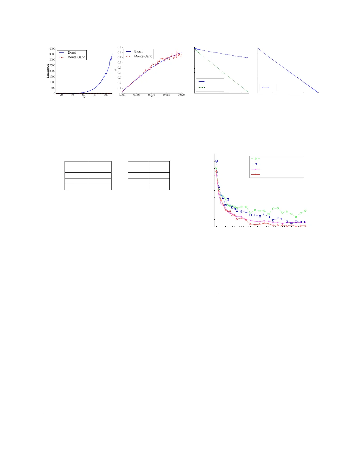
Sparsit yBo ost: A New Scoring F unction for Learning Ba y esian Net w ork Structure Eliot Brenner, ∗ Da vid Sontag Couran t Institute of Mathematical Sciences New Y ork Universit y Abstract W e give a new consistent scoring function for structure learning of Bay esian net works. In con trast to traditional approaches to score- based structure learning, such as BDeu or MDL, the complexity p enalt y that we pro- p ose is data-dependent and is given by the probabilit y that a conditional indep endence test correctly sho ws that an edge cannot ex- ist. What really distinguishes this new scor- ing function from earlier work is that it has the property of becoming computationally e asier to maximize as the amount of data in- creases. W e pro ve a p olynomial sample com- plexit y result, sho wing that maximizing this score is guarante ed to correctly learn a struc- ture with no false edges and a distribution close to the generating distribution, when- ev er there exists a Bay esian netw ork which is a perfect map for the data generating distri- bution. Although the new score can b e used with any searc h algorithm, w e giv e empirical results sho wing that it is particularly effec- tiv e when used together with a linear pro- gramming relaxation approach to Bay esian net work structure learning. 1 In tro duction W e consider a fundamental problem in statistics and mac hine learning: ho w can one automatically extract structure from data? Mathematically this problem can b e formalized as that of learning the structure of a Ba yesian netw ork with discrete v ariables. Ba yesian net works refer to a compact factorization of a m ul- tiv ariate probabilit y distribution, one-to-one with an ∗ Curren t Affiliation: Search & Algorithms, Shutter- stock Inc., New Y ork acyclic graph structure, in whic h the conditional prob- abilit y distribution of each random v ariable depends only on the v alues of its parent v ariables. One ap- plication of Ba yesian netw ork structure learning is for the disco very of protein regulatory netw orks from gene expression or flo w cytometry data (Sac hs et al. , 2005). Existing approac hes to structure learning follo w tw o basic metho dologies: they either search o ver struc- tures that maximize the li kelihoo d of the observ ed data (score-based methods), or they test for conditional in- dependencies and use these to constrain the space of p ossible structures. The former approac h leads to ex- tremely difficult combinatorial optimization problems, as the space of all p ossible Bay esian net works is expo- nen tially large, and no efficient algorithms are known for maximizing the scores. The latter approach gives fast algorithms but often leads to p oor structure re- co very because the outcomes of the indep endence tests can b e inconsistent, due to sample size problems and violations of assumptions. W e form ulate a new ob jectiv e function for structure learning from complete data which obtains the b est of b oth worlds: it is a score-based metho d, based pre- dominan tly on the likelihoo d, but it also makes use of conditional indep endence information. In particular, the new ob jectiv e has a “sparsit y b oost” corresp onding to the log-probability that a conditional indep endence test correctly shows that an edge cannot exist. W e sho w empirically that this new ob jectiv e substantially outperforms the previous state-of-the-art metho ds for structure learning. In particular, on synthetic distri- butions we find that it learns the true netw ork struc- ture with less than half the data and one tenth the computation. The contributions of this paper are the introduction of this new scoring function, a pro of of its consistency (w e show p olynomial sample complexit y), and a care- fully designed imp ortance sampling algorithm for ef- ficien tly computing the confidence scores used in the ob jective. F or b oth the pro of of sample complexity and the imp ortance sampling algorithm, w e develop several new results in information theory , constructing precise mappings b etw een a parametrization of distributions on tw o v ariables and m utual information, and charac- terizing the rate of conv ergence of v arious quan tities relating to m utual information. W e expect that man y of the techniques that w e dev elop ed will b e broadly useful b eyond Ba yesian netw ork structure learning. 2 Bac kground This pap er considers the problem of learning Bay esian net work structure from complete data (no hid- den v ariables or unobserv ed factors). Let X = ( X 1 , X 2 , . . . , X n ) b e a collection of random v ariables. F or reasons that w e explain in the next section, our results are restricted to the case when the v ariables X i are binary , i.e. V al( X i ) = { 0 , 1 } . F ormally , a Ba yesian netw ork ov er X is specified by a pair ( G, P ), where G = ( V , E ) is a directed acyclic graph (DA G) satisfying the following conditions: the no des V cor- respond to the v ariables X i ∈ X and E is such that ev ery v ariable is conditionally indep enden t of its non- descendan ts given its parents. The joint distribution can then be shown to factorize as P ( x 1 , . . . , x n ) = Q i ∈ V P ( X i = x i | X Pa( i ) = x Pa( i ) ), where Pa( i ) de- notes the paren t set of v ariable X i in the DA G G , and x Pa( i ) refers to an assignmen t to the paren ts. A Bay esian net work G is called an indep endence map (I-map) for a distribution P if all the (conditional) independence relationships implied by G are presen t in P . Going one step further, G is called a p erfect map for P if it is an indep endence map and the con- ditional indep endence relationships implied by G are the only ones presen t in P . By ω N (or in some con- texts, Y N ) we denote a sequence of observ ations of the random v ariables X , generated i.i.d. from an unkno wn Ba yesian netw ork ( G, P ), where G is a p erfect map for P . The problem that w e study is that of learn- ing the Bay esian net work structure and distribution ( G, P ) from the samples ω N . The simplest case of learning BN structure is when we ha ve tw o random v ariables, which we will call X A and X B . There are only tw o nonequiv alent BN structures: G 0 : X A X B ( “disconnected” ) , G 1 : X A − → X B ( “connected” ) . The structure learning problem in this case is to re- turn, based on ω N , a decision X A ⊥ ⊥ X B ( G 0 ) or X A 6⊥ ⊥ X B ( G 1 ). In other words, in this case, the structure learning problem is st rictly equiv alent to one case of hyp othesis testing , a w ell-studied and classic problem in statistics, sp ecifically testing the hypothe- sis of whether X A and X B are indep endent. In the case of three or more v ariables, the equiv alence no longer holds in any strict sense. Constr aint-b ase d appr o aches use the results of conditional independence tests to infer the mo del structure. These metho ds solve the structure learning problem sequentially by first learning the undirec ted skeleton of the graph, Skel( G ), and then ori enting the edges to obtain a DA G. Assum- ing that G is a p erfect map for P , if A is conditionally independent of B then we can conclude that neither A → B nor B → A can b e in G . It can b e shown that either A ’s parents or B ’s paren ts will b e a separat- ing set proving their conditional indep endence (there ma y b e others). Th us, if we make the key assump- tion that eac h v ariable has at most a fixed n umber of paren ts d , then this can yield a polynomial time al- gorithm for structure learning (Spirtes et al. , 2001; P earl & V erma, 1991). How ever, this approach has a num b er of draw backs: difficult y setting thresholds, propagation of errors, and inconsistencies. Let p = p ( ω N , A, B | s ) denote the empirical distribu- tion of A and B conditioned on an assignmen t S = s for S ⊆ V \{ A, B } , and marginalized ov er all of the other v ariables. The mutual information statistic, M I ( p ) = X a ∈ V al( A ) , b ∈ V al( B ) p ( a, b | s ) log  p ( a, b | s ) p ( a | s ) p ( b | s )  is a measure of the conditional indep endence of A and B conditioned on S = s . Giv en infinite data, tw o v ariables are indep enden t if and only if their mutual information is zero. Ho wev er, with finite data, mutual information is biase d aw ay from zero (Paninski, 2003). As a result, it can b e very difficult to distinguish b e- t ween indep endence and dep endence. An alternativ e approac h is to construct a scoring fun c- tion which assigns a v alue to ev ery possible structure, and then to find the structure which maximizes the score (Lam & Bacch us, 1994; Heck erman et al. , 1995). P erhaps the most p opular score is the BIC (Bay esian Information Criterion) score: S ψ 1 ( ω N , G ) = LL ( ω N | G ) − ψ 1 ( N ) · | G | . (1) Here, LL ( ω N | G ) is the log-lik eliho od of the data giv en G , | G | is the num b er of parameters of G , and ψ 1 ( N ) is a weigh ting function with the prop ert y that ψ 1 ( N ) → ∞ and ψ 1 ( N ) / N → 0 as N → ∞ . When ψ 1 ( N ) := log N 2 , the score, now called MDL, can b e theoretically justified in terms of Bay esian probabil- it y . In tuitively , we can explain the BIC/MDL score as a log-lik eliho od regularized by a c omplexity p enalty to keep fully connected mo dels (with the most pa- rameters) from alwa ys winning. Finding the struc- ture whic h maximizes the score is known to b e NP- hard (Chic kering, 1996; Chic kering et al. , 2004; Das- gupta, 1999). Heuristic algorithms hav e b een prop osed for maximizing this score, suc h as greedy hill-clim bing (Chic kering, 2002; F riedman et al. , 1999) and, more recen tly , by formulating the structure learning prob- lem as an in teger linear program and solving using branc h-and-cut (Cussens, 2011; Jaakk ola et al. , 2010). The running time of solving the integer linear pro- grams dramatically increases as the amoun t of data used for learning increases (see, e.g., Fig 4). This is coun ter-intuitiv e: more data should mak e the learning problem easier, not harder. The core problem is that as the amount of data increases, the likelih o o d term gro ws in magnitude whereas the complexity penalty shrinks. This is necessary to pro ve that these scoring functions are consisten t, i.e. that in the limit of infi- nite data the structure which maximizes the score in fact is the true structure. As a consequence, ho wev er, the score b ecomes very flat near the optim um with a large num b er of lo cal maxima, making the optimiza- tion problem extremely difficult to solve. 3 Sparsit yBo ost: A New Score for Structure Learning W e design a new scoring function for structure learning that is b oth consisten t and easy to solve regardless of the amount of data that is av ailable for learning. The k ey prop ert y that w e wan t our new scoring function to hav e is that as the amount of data increases, opti- mization b ecomes easier, not harder. When little data is av ailable, it should reduce to the existing scoring functions. Our approach is to add, to the BIC score, new terms deriv ed from statistical indep endence tests. Before in- troducing the new score w e provide some background on hypothesis testing. Let P denote the simplex of (join t) probabilit y distributions o ver a pair of random v ariables, and let P 0 denote the subset of pro duct dis- tributions: P 0 = { q ∈ P | M I ( q ) = 0 } . F or q / ∈ P 0 , the magnitude of M I ( q ) pro vides a measure of how far q is from the set of product distributions. F or η > 0, we define P η := { q | M I ( q ) ≥ η } . The testing pro cedure has ω N as input, n ull hypothesis H 0 (independence) for p ∈ P 0 , and alternativ e hypothesis H 1 for p ∈ P η . The T yp e I err or α N is defined as the probability of the test rejecting a true H 0 , the T yp e II err or β N is defined as the probabilit y of the test falsely accepting H 0 , and the p ower is defined as 1 − β N . The theory of Neyman-Pearson hypothesis testing for comp osite hypotheses tells us how to construct a hy- p othesis test of maximal p ower for any α N (Ho effd- ing, 1965; Dem b o & Zeitouni, 2009). In our set- ting, the test corresp onds to computing M I ( ω N ) := M I ( p ( ω N )) and deciding on H 1 if the test statistic ex- ceeds a threshold γ . Let β N ( γ ) denote the Type I I error of the Neyman-P earson test with threshold γ . W e prop ose using in our score the Type I I error of the test with threshold M I ( ω N ), β p η N ( M I ( ω N )) := Pr Y N ∼ p η { M I ( Y N ) ≤ M I ( ω N ) } , where p η is the M -pro jection of p ( ω N ) onto P η , that is, with H ( ·k· ) denoting the Kullback-Leibler divergence, p η := argmin p ∈P η H ( p ( ω N ) k p ) . (2) An intuitiv e explanation for the Type I I error is that β p η N ( γ ) is the probabilit y of obtaining a test statis- tic M I ( Y N ) , Y N ∼ p η , that is mor e extr eme , in the wr ong direction of independence, than the observed test statistic γ . On the one hand, if ω N ∼ p 0 ∈ P 0 , then with high probability the pow er of the test with threshold M I ( ω N ) approac hes 1 and β p η N ( M I ( ω N )) approac hes 0, exp onenti ally fast as N → ∞ ; on the other hand, if ω N ∼ p 1 ∈ P  , where  > η , then with high probability the pow er approache s 0 and β p η N ( M I ( ω N )) approaches 1, as N → ∞ . No w w e can state our new score for structure learning and explain its remaining features: S η ,ψ 1 ,ψ 2 ( ω N , G ) = LL ( ω N | G ) − ψ 1 ( N ) · | G | + ψ 2 ( N ) · X ( A,B ) / ∈ G max S ∈ S A,B ( G ) min s ∈ v al( S ) − ln h β p η N ( M I ( p ( ω N , A, B | s ))) i The first line is the BIC score. In the second line ψ 2 ( N ) is a w eighting function suc h that ψ 2 ( N ) / N → 0 as N → ∞ : ψ 2 ( N ) := 1 in the exp erimen ts. Each term in the sum is called a sp arsity b o ost . The sum con tains one sparsit y b o ost for each nonexistent edge ( A, B ) / ∈ G . If A ⊥ ⊥ B | ( S = s ), then the sparsit y b o ost is Θ( N ) as N → ∞ , and if A 6⊥ ⊥ B | ( S = s ), then it is O (1), and further, in that case the sparsit y b oost b ecomes insignificant compared to the LL term (since ψ 2 ( N ) / N → 0). Second, the sets S A,B ( G ), called sep ar ating sets , are certain subsets of the pow er set of V − { A, B } , which pro vide c ertific ates for statistic al r e c overy of G . More precisely , we hav e ( A, B ) / ∈ G , if and only if there is a witness S ∈ S A,B ( G ) suc h that A ⊥ ⊥ B | S . The most common wa ys of defining S A,B ( G ) are as follo ws: S A,B ( G ) = { S ⊂ V \{ A, B } | | S | ≤ d } , (3) S A,B ( G ) = { Pa G ( A ) \ B , P a G ( B ) \ A } . (4) The family of assignmen ts ( A, B , G ) 7→ S A,B ( G ) for all ( A, B ) ranging ov er distinct pairs of vertices and G o ver some family G of DA Gs, constitutes a c ol le ction of sep ar ating sets , denoted b y S . In order for A ⊥ ⊥ B | S to hold, we m ust ha ve A ⊥ ⊥ B | s , for every join t assignment s ∈ V al( S ). This is the reason for taking the minimum ov er s ∈ V al( S ) of the p ossible sparsity b oosts. The existence of just one S ∈ S A,B ( G ) suc h that A ⊥ ⊥ B | S suffices to rule out ( A, B ) as an edge in G . This is the reason for taking the maximum o ver S ∈ S A,B ( G ). The sparsit y b oost is O (1) for an ( A, B ) ∈ G , and Θ( N ) for an ( A, B ) / ∈ G . It remains to explain how to compute β p η N ( γ ) in the im- plemen tation of the score S η ,ψ 1 ,ψ 2 . According to the definition (2), p η is data-dep enden t, and this mak es it impractical to compute β p η N ( M I ( ω N )) quic kly enough for use in our algorithm. W e make an appro ximation b y fixing p η to b e a singl e “reference” distribution, with uniform marginals and satisfying M I ( p η ) = η . In the case when V al( X i ) = { 0 , 1 } , there are t wo such distri- butions. Namely , let p 0 denote the uniform distribu- tion, and let p 0 ( t ) =   1 4 + t 1 4 − t 1 4 − t 1 4 + t   for all t ∈  − 1 4 , 1 4  . (5) Clearly , p 0 ( t ) has uniform marginals. Consider the function M I ( p 0 ( t )) for t ∈  0 , 1 4  . On this inter- v al M I ( p 0 ( t )) is p ositiv e, increasing, and has range  0 , M I  p 0  1 4  . Thus for eac h η in the range, there is a unique parameter v alue t + η suc h that M I ( p 0 ( t + η )) = η . By symmetry , w e also hav e M I ( p 0 ( − t + η ))) = η ; fix p η := p 0 ( t + η ) . (6) W e compute t + η b y a binary search in the interv al  0 , 1 4  ; by (5) and (6) this suffices to compute p η , and has to b e done only once during the algorithm’s setup. Ha ving computed p η , w e can compute β p η N ( γ ) for many v alues of N , γ , and store them in a table. During the learning phase, we ev aluate β p η N ( M I ( ω N )) by interpo- lation. W e explain more details in Sec. 5. Related w ork . Our new score is similar to other “hy- brid” algorithms that use both conditional indep en- dence tests and score-based searc h for structure learn- ing, notably F ast 2010’s Greedy Relaxation algorithm ( Relax ) and Tsamardi nos e t al. 2006’s Max-Min Hill- Clim bing (MMHC) algorithm. The MMHC algorithm has tw o stages, first using indep endence tests to con- struct a skelet on of the Bay esian net work, and then p erforming a greedy searc h o ver orientations of the edges using the BDeu score. The Relax algorithm starts b y p erforming c onditional indep endence tests to learn constraints, follow ed b y edge orientation to pro- duce an initial mo del. After the first mo del has b een iden tified, Relax uses a local greedy search ov er pos- sible relaxations of the constrain ts, at eac h step choos- ing the single constrain t which, if relaxed, leads to the largest improv emen t in the score. Both of these al- gorithms separate the constraint- and score-based ap- proac hes into tw o distinct steps, in contrast to our approac h whic h directly incorp orates the conditional independence tests as a term in the score itself. The only other work that we are aw are of that has studied the incorp oration of reliabilit y of indep endence tests in score-based structure search is de Camp os (2006). Their ob jective function is v ery different from ours, comparing the empirical mutual information to its exp ected v alue assuming indep endence (using the χ 2 distribution). In con trast to de Camp os’s MIT score, the SparsityBoost score is consistent, prov ably able to recov er the true structure. Imp ortance of using Type II error. T o our knowl- edge, all previous approac hes for Bay esian netw ork structure learning use the Type I error α N in assessing the reliability of an indep endence test, whic h is asymp- totically giv en b y the χ 2 distribution. A relativ ely high threshold needs to be specified in order to preven t the false rejection of indep endence and to correct for m ulti- ple hypothesis testing. One of our key contri butions is to show how to use β N , the Type I I error. Minimizing the T yp e II err or is essential b e c ause we want to err on the side of c aution , only having a large sparsit y bo ost if w e are sure that the corresponding edge does not ex- ist. Type I errors, on the other hand, can b e corrected b y the part of the ob jectiv e corresponding to the BIC score. If we had instead used the T yp e I error prob- abilit y within our score, it would hav e corresponded to a dependence bo ost rather than independence, and w ould b e fo oled if w e failed to find a go od separating set (e.g., for computational reasons). 4 P olynomial Sample Complexity of the Sparsit yBo ost Score 4.1 Statemen t of Main Results In this section, w e prov e the consistency of the Spar- sit yBo ost score. In order to state our main results, we need to define certain additional parameters. First, there is a (small) p ositiv e integer, d , which b ounds the in-degree of all vertices in G . The family of BNs on n v ertices satisfying this condition is called G d . Second, w e formalize the notion of the minimal edge strength  in G . Define S A,B ( G d ) := [ G ∈G d S A,B ( G ) . Recall that the witness sets in S provide certificates for statistical recov ery of G . W e quantify the edge strength of ( A, B ) ∈ G with resp ect to S A,B ( G d ), i.e. the amount of dep endence even after conditioning, b y  (( A, B ) , S A,B ( G d )) := min S ∈ S A,B ( G d ) max s ∈ V al( S ) M I ( p ( A, B | s )) Then, let  =  ( G ) = min ( A,B ) ∈ G  (( A, B ) , S A,B ( G d )). Next, we need the notion of an err or toler anc e ζ > 0, whic h in turn follows from a notion of a G 0 ∈ G d b eing ζ -far from the true net work ( G, P ). F or any G 0 ∈ G d , define the probabilit y distribution p G 0 ,P o ver X to b e the distribution which factors according to G 0 and minimizes the KL-divergence from P , i.e. p G 0 ,P := argmin Q : G 0 is an I-map for Q H ( P k Q ) . W e call H ( P k p G 0 ,P ) the div ergence of P from G 0 , and if H ( P k p G 0 ,P ) > ζ w e say that G 0 is ζ -far from ( G, P ) . In Theorem 1(a) w e set an error tol- erance of ζ , which is to say that w e sp ecify that our learning algorithm should rule out all G 0 whic h are ζ -far from ( G, P ). Finally , we need m , the (m aximum) in verse probability of an assignment to a separating set. More precisely , for any A, B ∈ V 2 , A 6 = B , and S ∈ S A,B ( G d ), let m P ( S ) := max s ∈ V al( S ) [ P ( S = s )] − 1 . Then let m = m P ( G, G d , S ) = max ( A,B ) ∈ G max S ∈ S A,B ( G d ) m P ( S ) . (7) F or all ( A, B ) / ∈ G , there will b e at least one witness S ∈ S A,B ( G ) such that A ⊥ ⊥ B | S . Let ˆ S P (( A, B ) , G ) := argmin S ∈ S A,B ( G ) : A ⊥ ⊥ B | S m P ( S ) . Finally , let ˆ m P ( G, S ) := max ( A,B ) / ∈ G m P ( ˆ S P (( A, B ) , G )) . (8) Theorem 1 Supp ose that ( G, P ) ∈ G d is a Bayesian network of n binary r andom variables and G is a p er- fe ct map for P . Set S A,B ( G ) = { S ⊂ V \{ A, B } | | S | ≤ d } . Assume that ( G, P ) ∈ G d has minimal e dge str ength  > 0 , and minimal assignment pr ob abilities m , as define d in (7) and ˆ m P ( G, S ) , as define d in (8) . Fix η = λ for λ ∈ (0 , 1) , an err or pr ob ability δ > 0 , and a toler anc e ζ > 0 . L et S η denote our sc or e S η ,ψ 1 ,ψ 2 for ψ 1 ( N ) := κ log ( N ) and ψ 2 ( N ) = 1 . L et ω N b e a se quenc e of observations sample d i.i.d. fr om P . (a) Ther e is a function N ( , m, n ; δ, ζ ; η , κ ) in ˜ O  max  log( n ) m  2 , n 2 ζ 2  log 1 δ  as , ζ , δ → 0 + , n, m → ∞ , such that for al l N > N ( , m, n ; δ, ζ ; η , κ ) , with pr ob ability 1 − δ , we have S η ( G, ω N ) > S η ( G 0 , ω N ) , for al l G 0 ∈ G d which ar e ζ -far fr om G . (b) Then ther e is a function N ( , m, ˆ m P , n ; δ ; η , κ ) in ˜ O  max  log( n ) m  2 , n 2 ˆ m 2 P  2  log 1 δ  as , δ → 0 + , n, m, ˆ m P → ∞ , such that for al l N > N ( , m, ˆ m P , n ; δ ; η , κ ) , with pr ob ability 1 − δ , we have S η ( G, ω N ) > S η ( G 0 , ω N ) , for al l G 0 ∈ G d such that Skel( G 0 ) 6⊆ Sk el( G ) . In order to explain the significance of this result, it is helpful to relate it to three representativ e sample complexit y results in the literature: H ¨ offgen (1993), F riedman & Y akhini (1996), Zuk et al. (2006). The result of Zuk et al. differs from the other tw o and from our result b ecause it only giv es conditions for the (BIC) score of G to beat that of an individual comp et- ing net work G 0 , not a family , such as G d . The main difference betw een H ¨ offgen and F riedman & Y akhini is that, like our result, H ¨ offgen assumes that the com- p eting net wor k lies in G d and ac hieves a sample com- plexit y that is p olynomial in n = card( V ), while F ried- man & Y akhini puts no restriction on the in-degree of comp eting net works, and obtains complexity that is exponential in n . Our result and Zuk et al. differ from b oth H ¨ offgen and F riedman & Y akhini in that w e prov ide guaran tees for learning the correct DA G structure G (or at least a G without false edges), not just a distribution P 0 whic h is ζ -close to P . F or this reason, only our paper and Zuk et al. need to define a minimal edge strength as a parameter, whereas for H ¨ offgen and F riedman & Y akhini the main parameter is the error tolerance ζ , whic h they call  . 4.2 Ov erview of Pro ofs The pro of of Theorem 1 consists of showing that for all sufficien tly large N we can find a (probable) low er b ound on the sc or e differ enc e , S η ( G, ω N ) − S η ( G 0 , ω N ) , G, G 0 ∈ G d , ω N ∼ G. (9) The score difference breaks do wn into a sum of the follo wing terms: (a) The difference of log-likelihoo d terms, LL ( G, ω N ) − LL ( G 0 , ω N ). (b) The difference of complexity p enalties, κ log( N )( | G 0 | − | G | ). (c) F or each distinct pair of vertices A, B ∈ V suc h that neither G nor G 0 has ( A, B ) as an edge, the difference of the sparsity b o osts in the ob jective functions of G and G 0 , for that nonexisten t edge. (d) F or each true e dge ( A, B ) ∈ G missing from G 0 , the negativ e of the sparsit y b o ost for ( A, B ) / ∈ G 0 . (e) F or each false e dge ( A, B ) 6∈ G presen t in G 0 , the (p ositiv e) sparsit y b o ost for ( A, B ) / ∈ G . With the choice of S in the Theorem, S A,B ( G 0 ) = S A,B ( G ) for all A, B ∈ V 2 , which implies that (c) is exactly 0. F urthermore, (b) is clearly O (log N ) for G, G 0 ∈ G d , while b oth (a) and (e) will turn out to b e Θ( N α ) for α > 0, so that (b) has only minor impact on the sample complexit y . So we will fo cus on how to estimate (a), (d), and (e). Conceptually , estimating each of these terms calls for the same typ e of r esult : a c onc entr ation lemma stating ho w quickly the empirical LL ( · , ω N ) (for (a)), respectively M I ( ω N , A, B | s ) (for (d) and (e)) con- v erges to the “ideal” coun terpart LL ( I ) ( · , P ), resp ec- tiv ely M I ( P , A, B | s ). In fact, both of the latter consist of a p olynomial in n num b er of terms (whic h is where w e use the hypothesis G ∈ G d ) of the form p log p for parameters p of certain Bernoulli random v ariables. Prop osition 1 L et p ∈ (0 , 1) b e given and X ( p ) the Bernoul li r andom variable with p ar ameter p . L et ˆ , δ ≥ 0 b e given. F or Y N ∼ p , denote the empiric al p ar ameter p Y N by ˜ p N . Then ther e is a function N (ˆ , δ ) ∈ O  1 ˆ   2 log 1 δ ! , (10) as ˆ , δ → 0 + with the pr op erty that for N > N ( ˆ , δ ) , Pr ( | ˜ p N log ˜ p N − p log p | < ˆ  ) ≥ 1 − δ. Proposition 1 impro ves sligh tly on Lemma 1 in H ¨ offgen (1993), by replacing ˜ O ( · ) with O ( · ) in (10). A k ey feature of Proposition 1, for obtaining our con- cen tration results for LL and M I is that (10) is in- dependent of the Bernoulli parameter p . F rom the concen tration result for LL , we can show that (a) is with high probability p ositiv e and larger than N ζ / 3, for all G 0 whic h are ζ -far from G and for sufficiently large N . F rom the concentrat ion result for M I we can sho w that a sparsit y b o ost from a true edge is b ounded ab o ve by a constan t for sufficiently large N (linear in m ). So the negative con tribution of (d) is b ounded. These b ounds suffice to pro ve Theorem 1(a). In the pro of of Theorem 1(b), from the concen tra- tion result for LL , we can show that (a) is with high probabilit y larger than a constan t times − n p log( n ) N . F urthermore, a sparsity bo ost from a false edge is Ω(Γ( η ) N ), where the speed Γ( η ) of the linear growt h is on the order of η 2 as η → 0 + . T o show the latter, w e first apply Prop osition 1, giv en a witness, to prov e that M I ( ω N , A, B | s ) is (likely) less than η / 2. Second, using a Chernoff b ound, we sho w that − log β p η N ( γ ) is Ω( η 2 N ) for γ less than η / 2. So, with high probabilit y the p ositiv e contribution of (e) even tually ov erwhelms an y negativ e con tribution of (a). The techniques deriv ed from the Chernoff b ound yield a v ersion of Theorem 1(b) with an exp onent of 4 on the  in the denominator of the term n 2 ˆ m 2 P / 2 . T o impro ve the exp onen t to 2, w e need a strengthened result on the linear gro wth of a sparsit y b oost from a false edge, in which the sp eed Γ( η ) is on the order of only η instead of η 2 , as η → 0 + . W e hav e to use a new metho d derived from Sano v’s Theorem instead of Chernoff ’s Bound. T o our knowl- edge, the wa y we use Sanov’s Theorem to study the concen tration of mutual information is a no vel contri- bution to information theory . F or all of the following w e are assuming that V al( X i ) = { 0 , 1 } for all X i ∈ V so that P is the space of probabilit y distributions ov er the alphab et { 0 , 1 } 2 . W e hav e already , in (5), given a parameterization of the path of distributions of uni- form marginals in P . W e now generalize (5) and the asso ciated parameterization by defining p ( p A, 0 , p B , 0 , t ) :=  p A, 0 p B , 0 + t p A, 1 p B , 0 − t p A, 0 p B , 1 − t p A, 1 p B , 1 + t  (11) where p A, 1 := 1 − p A, 0 and p B , 1 := 1 − p B , 0 . When ( p A, 0 , p B , 0 ) ranges ov er [0 , 1] 2 and t ov er ( t min , t max ) (an interv al dep ending on p A, 0 , p B , 0 ), (11) parameter- izes the whole space P . Since the t parameter is a measure of ho w far p is from P 0 , it is not surprising that we can derive formulas relating t to √ M I . In order to carry this out, we consider the function M I ( p ( p A, 0 , p B , 0 , t )) as a function of t and carefully study the T a ylor series expansion of this function around the basepoint t = 0. The reason for preferring the t parameter to M I itself is that b y means of Sano v’s Theorem and Pinsk er’s In- equalit y , we obtain a very general result which bounds − log β p η N ( γ ) from b elo w b y N times the squared L ∞ - distance of p η from a distribution q γ . More sp ecifically , defining the complemen t of P γ b y A γ := { p ∈ P | M I ( p ) ≤ γ } , (12) the distribution q γ is defined as the I-pro jection of p η on to A γ . W e would lik e to relate k p η − q γ k ∞ to | M I ( p η ) − M I ( q γ ) | = | η − γ | , and the t -parameters act as an effectiv e intermediary , b ecause it is easy to show that k p η − q γ k ∞ is on the order of | t + η − t + γ | , where t + γ is the t -parameter of q γ . Applying the relation of the preceding paragraph b et ween t and √ M I , we obtain a b ound, from b elo w, of − log β p η N ( γ ) by something on the order of ( √ η − √ γ ) 2 N . 5 Computation of β v alues Exact computation. Here we giv e an exact for- m ula for β p η N ( γ ) using the Method of T yp es (Cov er & Thomas, 2006, Chapter 11). Denoting the en tries of p η ∈ P by ( p 0 , 0 , p 0 , 1 , p 1 , 0 , p 1 , 1 ), we hav e β p η N ( γ ) = X Y N 1 Y i,j =0 p T i,j ( Y N ) i,j 1 [ M I ( Y N ) ≤ γ ] , where T i,j ( Y N ) is the num ber of observ ations of ( i, j ) in the sampled sequence Y N of length N . Consider the set T N of length-4 v ectors of nonnegativ e in tegers ( T 0 , 0 , T 0 , 1 , T 1 , 0 , T 1 , 1 ) summing to N . Ev ery T ∈ T N corresponds one-to-one with a distribution p T ∈ P (obtained by dividing ev ery entry in T b y N ). Let | T | denote the num b er of sequences Y N corresponding to type T . Then it is not difficult to see that | T | is giv en b y a m ultinomial co efficient and that β p η N ( γ ) = X T ∈T N | T | 1 Y i,j =0 p T i,j i,j 1 A γ ( p T ) , (13) where 1 A γ is the c haracteristic function of A γ (see Eq. 12). W e can use (13) to exactly compute β p η N ( γ ), but b ecause of the summation ov er T N the running time of this algorithm is O ( N 3 ), which will not scale to the range of N we need for our experiments. Mon te Carlo computation. In place of exact cal- culation, we estimate β p η N b y means of Monte Carlo in tegration, using imp ortance sampling of the domain to reduce the v ariance. In order to implement this, we first observ e that (13) is essentially a Riemann sum for a definite integral, so that we may replace the summa- tion with an in tegral. Second, the in tegrand w e ini- tially obtain in this manner has n umerous discon tinu- ities, b ecause of th e | T | factor. It mak es the next steps easier to implement if we replace | T | with a (sligh tly larger) contin uous approximation (Csiszar & K ¨ orner, 2011, p. 39). W e finally obtain the following in tegral whic h appro ximates β p η N ( γ ) giv en in (13):  N 2 π  ( | X |− 1) / 2 Z P e − N H ( q k p η ) 1 Y i,j =0 q − 1 2 i,j 1 A γ ( q ) d q . F or the Mon te Carlo integration w e use an imp ortance sampling scheme based on the following idea: the in- tegrand is largest when H ( q k p η ) is small and q ∈ A γ , and so it should b e strongly concentrated around q γ (the I-pro jection of p η on to A γ ). W e ha ve an un- pro ven conjecture, supp orted by numerical evidence, that q γ = p γ := p 0 ( t + γ ) (the unprov en part of this is that q γ has uniform marginals) for η less than appro x- imately 0 . 1109. The importance sampling algorithm samples p oints p ∈ P i.i.d., fa voring p oin ts near p γ . W e use the parameterization (11) of P and sample the parameters p A, 0 , p B , 0 & t indep enden tly according to Gaussian distributions. F or the selection of the tw o marginals, we use iden tical Gaussians centered at 1 2 and b ecoming more concentrat ed (exp onen tially fast) around their mean as N → ∞ . F or the t parame- ter, we use use a third Gaussian centered at t + γ . F or eac h ( N , γ ) we determine the concent ration of the third Gaussian by sampling the integrand along the path p  1 2 , 1 2 , t  , in the segmen t (0 , t + γ ). Since we cannot p ossibly tabulate β p η N ( ω N ) for ev- ery empirical sequence that migh t arise, we tabulate β p η N ( γ ) for N , γ in a strategically c hosen grid of v alues, and during the learning phase w e interpolate or extrap- olate (as the need arises) from these tabulated v alues. W e in terp olate/extrapolate − ln β p η N ( γ ) line arly in the statistics N and H ( p γ k p η ). Sano v’s Theorem gives heuristic support to this procedure, but ultimately our justification for this pro cedure rests on the empirical results presented in Section 6 below. 6 Exp erimen tal Results Computing the confidence measure. In Figure 1 w e present several empirical results that help to justify our metho ds for calculating β p η N ( γ ), our new measure of the reliability of an independence test. First, in (a), w e show that using the metho d of summing o ver t yp es to calculate β p η N ( γ ) has a running time whic h is O ( N 4 ), whereas the Mon te Carlo metho d explained in Section 5 is O (1) as N → ∞ . Thus, although it is feasible to pre-compute β p η N ( γ ) for small v alues of N , exact calculation is impractical for N muc h larger than 200. As for the accuracy of the Mon te Carlo estimation, the table in Figure 2 shows that for very small N , e.g. N < 50, some m ultiplicative errors for our method of ≈ 30% are observed, but by the time we reach N = 100, the errors are consisten tly < 10%. Figure 1(b) sho ws that, for N = 200, the Mon te Carlo estimate has a consisten tly small error ov er the range of γ . The linear in terp olation pro cedure for obtaining ln β p η N ( M I ( ω N )) from the pre-computed tables of ln β p η N ( γ ) receives heuristic supp ort from Sano v’s The- orem; it receives empirical supp ort from Figure 1(c) (resp. (d)), whic h sho ws that the dep endence of ln β p η N ( γ ) on N (resp., H ( p γ k p η )), assuming all other inputs are fixed, is roughly linear. Sample Complexity . In this section w e study the accuracy of our learning algorithm as a function of the amoun t of data w e provide it. W e compare our algorithm to tw o baselines: BIC and Max-Min Hill- Clim bing. BIC is equiv alent to our score without 20 40 60 80 100 N 0 500 1000 1500 2000 2500 3000 3500 4000 seconds Exact Monte Car lo 0 . 000 0 . 005 0 . 010 0 . 015 0 . 020 γ 0 . 1 0 . 2 0 . 3 0 . 4 0 . 5 0 . 6 0 . 7 0 . 8 0 . 9 β Exact Monte Car lo 0 2000 4000 6000 8000 10000 N 10  20 10  16 10  12 10  8 10  4 10 0  (0 . 005)  (0 . 001) 0 . 0000 0 . 0025 0 . 0050 0 . 0075 0 . 01 00 H ( p  k p ⌘ ) 10  38 10  32 10  26 10  20 10  14 10  8 10  2  (a) (b) (c) (d) Figure 1: Computation of β p η N . All results shown are for η = 0 . 01. (a) Running time of the exact algorithm to compute β p η N gro ws cubically in N , but for Monte Carlo approximation remains constan t (results shown for γ = 0 . 005 and 0 . 001 com bined). (b) Mon te Carlo estimate of β p η N ( γ ) for fixed η , N = 200. (c) Exponentia l deca y of β p η N ( γ ) in N for fixed γ . (d) Exponential decay of β p η N ( γ ) as a function of KL-div ergence H ( p γ k p η ), as γ is v aried, for large N = 9000. γ N 0 . 001 0 . 005 20 12.20% 29.15% 30 24.65% 1.18% 40 39.77% 7.07% 50 2.45% 4.88% 60 3.52% 0.30% γ N 0 . 001 0 . 005 70 1.03% 3.59% 80 9.06% 4.13% 90 0.77% 4.05% 100 1.01% 0.03% 110 2.27% 3.01% Figure 2: Multiplicativ e error of Mont e Carlo approxima- tion, | β p η N − ˆ β p η N | /β p η N , for η = 0 . 01 as N , γ v ary . the sparsity b o ost terms. MMHC is state-of-the-art in terms of b oth speed and quality of recov ery , and has been shown to outperform most other constrain t- based approaches (Tsamardinos et al. , 2006). As w e discussed earlier, MMHC is also a hybrid algorithm, using b oth conditional indep endence tests and score- based search. W e use the implementation of MMHC pro vided by the authors as part of Causal Explorer 1.4 (Aliferis et al. , 2003), with the default parameters. 1 W e use an integer linear program to exactly solv e for the Bay esian netw ork that maximizes the BIC or Sparsit yBo ost scores (Jaakk ola et al. , 2010; Cussens, 2011). T o solv e the ILP , we use Cussens’ GOB- NILP 1.2 soft ware together with SCIP 3.0 (Ac hter- b erg, 2009). Conv eniently , since the sparsity b oost terms in our ob jective can be subsumed into the par- en t set scores, w e can use these off-the-shelf Ba yesian net work solvers without an y modification. The data that we use for learning is sampled from syn thetic distributions based on the Alarm netw ork structure (Beinlic h et al. , 1989). The Alarm net- w ork has 37 v ariables, 46 edges, and a maxim um in-degree of 4. In our syn thetic distributions, ev- ery v ariable has only t wo states, and its conditional probabilit y distribution is given by a logistic function, p ( X i = 1 | x Pa( i ) ) = 1 / (1 + e − ~ θ i · x Pa( i ) − u i ). W e sam- 1 Threshold for χ 2 test of . 05 and Dirichlet h yp erparam- eters equal to 10. V arying these did not improv e results. 0 500 1000 1500 2000 2500 3000 3500 4000 0 5 10 15 20 25 30 35 40 45 50 Number of samples Structural Hamming Distance MMHC BIC SparsityBoost eta=0.04 SparsityBoost eta=0.01 Figure 3: Comparison of the sample complexit y of MMHC, BIC, and our new Sparsit yBo ost ob jective. Each point is the av erage of the SHD of the learned netw ork from truth for 10 synthetic distributions. pled 10 differen t distributions, with parameters dra wn according to θ ij ∼ U [ − . 5 , . 5] + 1 4 N (0 , 1) for j ∈ Pa( i ) and u i ∼ 1 4 N (0 , 1). F or eac h v alue of N , a new set of N samples were dra wn from the corresp onding syn- thetic distribution. The results shown are the a verage for each of these 10 synt hetic distributions. W e use S A,B ( G ) from Eq. 3 with d = 2, en umerating o ver all separating sets of size at most tw o. Larger separating sets are less useful because they lead to a smaller  , less data, and more computation to cre- ate the ob jectiv e. In the Alarm net work, for ev ery ( A, B ) 6∈ G there is a separating set S such that | S | ≤ 2 and A ⊥ B | S . Regardless, if a separating set for an inexisten t edge cannot b e found, our score simply re- duces to the BIC score, so no harm is done. Our results are shown in Figure 3. W e measure the qualit y of structure recov ery using the Structural Ham- ming Distance (SHD) b et ween the partially directed acyclic graphs (PDA G) representing the equiv alence classes of the true and learned netw orks (Tsamardi- nos et al. , 2006). The SHD is defined as the n umber 0 1000 2000 3000 4000 5000 6000 7000 8000 0 200 400 600 800 1000 1200 1400 Number of samples Running time (seconds) BIC SparsityBoost eta=0.01 MMHC Figure 4: T otal running time to learn a Bay esian net- w ork from data for BIC, SparsityBoost, and MMHC. W e maximize the BIC and Sparsit yBo ost scores by solving an in teger linear program to optimality . of edge additions, deletions, or rev ersals to make the t wo PD AGs matc h. The plots for SparsityBoost with η = 0 . 005 and η = 0 . 02 (not shown) are nearly iden- tical to that of η = 0 . 01. SparsityBoost consistently learns b etter structures than MMHC or BIC, an d often p erfectly reco vers the netw orks after only 1600 sam- ples. SparsityBoost obtains a smaller av erage error with 3000 samples than BIC do es with 6000, repre- sen ting a more than 50% reduction in the num b er of samples needed for learning. W e also found that the Sparsit yBo ost results had substan tially less v ariance than either BIC or MMHC. Our theoretical results only guarantee exact recov ery when η <  . F or each of the synthetic distributions w e computed  ( A, B ) for all of the edges ( A, B ) in the true structure (see Sec. 4.1 for definition). The mini- m um of these, that is to say  , ranged from . 000028 to . 0047, which i s in fact smal ler than the largest v alue of η considered in our exp erimen ts (.005). Despite this, w e obtained excellent empirical results for Sparsity- Bo ost with η ∈ { . 005 , . 01 , . 02 } . This ma y b e partially explained by the aver age v alue of  ( A, B ) b eing . 062. Ev en when we push η to b e as high as . 04, Sparsity- Bo ost con verges to an a verage SHD of at most 3 (see Fig. 3). Thus, our new ob jective app ears to b e partic- ularly robust to choosing the wrong v alue of η . Running Time. W e sho w the running time of our new ob jective compared to BIC in Figure 4. The fig- ure sho ws the total time, whic h includes b oth the time to compute the score of all parent sets and the time to solv e the ILP to optimality . These results confirm our h yp othesis that the new score would b e substantially easier to optimize. W e found that the linear program- ming relaxation for Sparsit yBo ost (with η = 0 . 01) w as tigh t on ne arly al l instances: branc h-and-b ound did not need to b e p erformed. Once the Sparsit yBo ost ob jective has b een computed, the ILP is solved within 6 seconds in ev ery single instance. The timing exp eriments reported in this section were p erformed on a single core of a 2.66 Ghz Intel Core i7 pro cessor with 4 GB of memory . MMHC’s av erage running time was less than 8 seconds for all sample sizes. MMHC is significan tly faster because it quickly prunes edges that cannot exist and in its second step uses a greedy (rather than exact) optimization algo- rithm for score-based search. 7 Discussion Our ap proach maintains the adv antages of other score- based approaches to structure learning, suc h as the abilit y to find the K -b est Bay esian net works and ease of introducing additional constraints (e.g., from inte r- v entional data). In order to optimize our score, virtu- ally any optimization pro cedure can b e used. Since the ILP is easy t o solv e, this suggests that greedy struc ture searc h ma y also b e able to easily find the best-scoring Ba yesian netw ork under the Sparsit yBo ost score. One sub ject for future inv estigations is to generalize and sharp en our results in v arious wa ys. Using a simi- lar construction for p η , w e b eliev e it should b e possible to extend our score and pro of of consistency to non- binary v ariables. W e also b elieve it will b e p ossible to eliminate the dependence of N ( , m, ˆ m P , n ; δ, ζ ; η , κ ) in b oth parts of Theorem 1 on the parameter m , leaving only the dep endence on ˆ m P in part (b), which is in some cases muc h smaller than m . Another issue to b e explored as a future line of in v esti- gation is the choice of p η in our measure of reliabilit y , β p η N ( γ ). The o verall motiv ation for β p η N ( γ ) is to capture the probabilit y of Type I I error of a statistical test with independent distributions P 0 as the n ull hypothesis H 0 and all distributions P η as the alternative h yp othesis H 1 . The choice of uniform marginals for p η represen ts an exp edien t choi ce, providing an ob jective function that is manageable to implemen t and compute, yet still has a reasonable theoretical and empirical sam- ple complexity . Better results might b e obtained by setting the marginals of p η to approximate those of p ( ω N ). More generally , one can contemplate incorpo- rating v arious other statistically deriv ed probabilities in to the ob jective function. This leads to the broader p oin t that ob jectiv e func- tions, and the optimization of them ov er discrete spaces of structures, are ubiquitous throughout com- puter science and statistics. Our work suggests a new paradigm for incorp orating information from “classi- cal” hypothesis tests into the ob jectiv e functions used for mac hine learning. This new paradigm pro vides b oth computational and statistical efficiency . References Ac hterberg, T obias. 2009. SCIP: Solving constraint inte- ger programs. Mathematic al Pr o gramm ing Computation , 1 (1), 1–41. Aliferis, Constantin F., Tsamardinos, Ioannis, Statniko v, Alexander R., & Brown, Laura E. 2003. Causal Ex- plorer: A Causal Probabilistic Netw ork Learning T o olkit for Biomedical Disco very . Pages 371–376 of: METMBS . Beinlic h, I. A., Suermondt, H. J., Chav ez, R. M., & Coop er, G. F. 1989. The ALARM Monitoring System: A Case Study with Two Probabilistic Inference T echniques for Belief Netw orks. Pages 247–256 of: Pro c e e dings of the 2nd Eur op e an Confer enc e on Artificial Intel ligenc e in Me dicine . Springer-V erlag. Chic kering, D. 1996. Learning Bay esian Netw orks is NP- Complete. Pages 121–130 of: Fisher, D., & Lenz, H.J. (eds), L e arning fr om Data: A rtificial Intel ligenc e and Statistics V . Springer-V erlag. Chic kering, D. 2002. Learning Equiv alence Classes of Ba yesian-Net work Structures. Journal of Machine L e arning Res ear ch , 2 , 445–498. Chic kering, D., Heck erman, D., & Meek, C. 2004. Large- Sample Learning of Ba yesian Netw orks is NP-Hard. Journal of Machine L e arning R ese ar ch , 5 , 1287–1330. Co ver, T.M., & Thomas, J.A. 2006. Elements of informa- tion the ory . John Wiley & Sons. Csiszar, I., & K ¨ orner, J. 2011. Information theo ry: c o ding the or ems for discr ete memoryless systems . Cambridge Univ ersity Press. Cussens, James. 2011. Ba yesian netw ork learning with cutting planes. Pages 153–160 of: Pro c e e dings of the Twenty-Seventh Confer enc e Annu al Confer ence on Un- c ertainty in Artificial Intel ligenc e (UAI-11) . Corv allis, Oregon: A UAI Press. Dasgupta, S. 1999. Learning p olytrees. In: Pr o c. of the 15th Confer enc e on Uncer tainty in Artificial Intel- ligenc e . de Campos, Luis M. 2006. A Scoring F unction for Learning Ba yesian Netw orks based on Mutual Information and Conditional Indep endence T ests. J. Mach. L e arn. R es. , 7 (Dec.), 2149–2187. Dem b o, A., & Zeitouni, O. 2009. L ar ge deviations tech - niques and applic ations . V ol. 38. Springer. F ast, A. 2010. Le arning the structur e of Bayesian networks with c onstr aint satisfaction . Ph.D. thesis, Universit y of Massac husetts Amherst. F riedman, N., & Y akhini, Z. 1996. On the Sample Com- plexit y of Learning Bay esian Netw orks. In: Pr o c. of the 12th Confer enc e on Unc ertainty in Artifici al Intel li- genc e . F riedman, Nir, Nac hman, Iftach, & P e’er, Dana. 1999. Learning Ba yesian Net wo rk Structure from Massiv e Datasets: The “Sparse Candidate” Algorithm. Pages 206–215 of: UAI . Hec kerman, D., Geiger, D., & Chick ering, D. M. 1995. Learning Ba yesian Net works: The Combination of Kno wledge and Statistical Data. Machine L e arning , 20 (3), 197–243. Av ailable as T ec hnical Rep ort MSR- TR-94-09. Hoeffding, W. 1965. Asymptotically optimal tests for m ultinomial distributions. The Annals of Mathematic al Statistics , 369–401. H ¨ offgen, K.U. 1993. Learning and robust learning of pro d- uct distributions. Pages 77–83 of: Pr oc e e dings of the sixth annual c onfer enc e on Computational le arning the- ory . AC M. Jaakk ola, T ommi, Son tag, Da vid, Glob erson, Amir, & Meila, Marina. 2010. Learning Bay esian Netw ork Struc- ture using LP Relaxations. Pages 358–365 of: Pr o- c e e dings of the Thirte enth International Confer enc e on Ar tificial Intel ligenc e and Statistics (AI-ST A TS) , vol. 9. JMLR: W&CP . Lam, W ai, & Bacch us, F ahiem. 1994. Learning Bay esian Belief Netw orks: An Approach Based on the MDL Prin- ciple. Computational Intel ligenc e , 10 , 269–294. P aninski, Liam. 2003. Estimation of entrop y and m utual information. Neur al Comput. , 15 (6), 1191–1253. P earl, Judea, & V erma, Thomas. 1991. A Theory of In- ferred Causation. Pages 441–452 of: KR . Sac hs, Karen, Perez, Omar, P e’er, Dana, Lauffen- burger, Douglas A., & Nolan, Garry P . 2005. Causal Protein-Signaling Netw orks Derived from Multiparame- ter Single-Cell Data. Science , 308 (5721), 523–529. Spirtes, P ., Glymour, C., & Sc heines, R. 2001. Causation, Pr e diction, and Se ar ch, 2nd Edition . The MIT Press. Tsamardinos, I., Brown, L. E., & Aliferis, C. F. 2006. The Max-Min Hill-Climbing Bay esian Netw ork Struc- ture Learning Algorithm. Machine L e arning , 65 (1), 31– 78. Zuk, Or, Margel, Shiri, & Doman y , Eytan. 2006. On the Num b er of Samples Needed to Learn the Correct Struc- ture of a Ba yesian Netw ork. In: UAI . AUAI Press.