Latent Fisher Discriminant Analysis

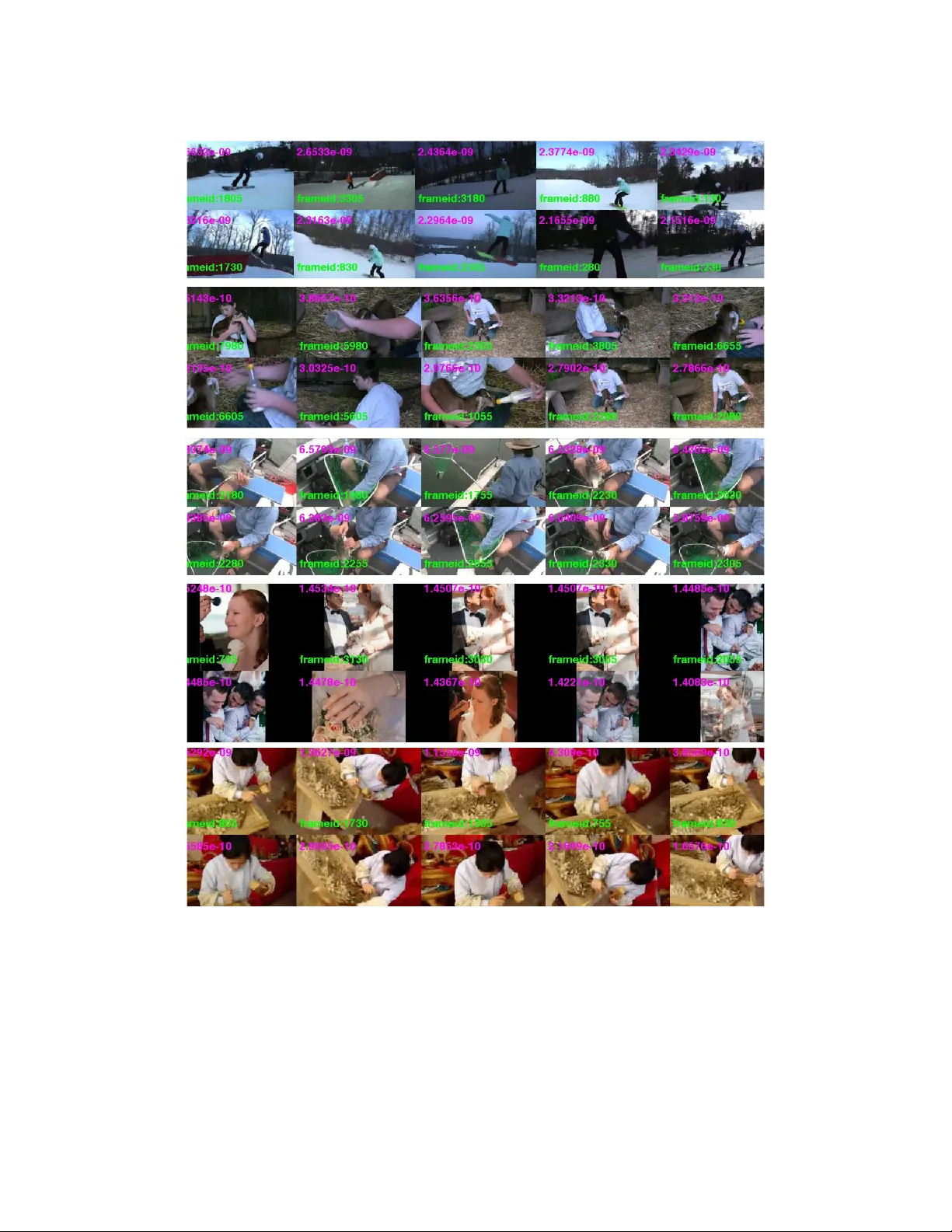
Latent Fisher Discriminant Analysis Gang Chen Department of Computer Science and Engineering SUNY at Buf falo gangchen@buffalo.edu September 24, 2013 Abstract Linear Discriminant Analysis (LD A) is a well-known method for dimensionality reduction and clas- sification. Previous studies have also extended the binary-class case into multi-classes. Howe v er , many applications, such as object detection and keyframe extraction cannot provide consistent instance-label pairs, while LD A requires labels on instance lev el for training. Thus it cannot be directly applied for semi-supervised classification problem. In this paper , we ov ercome this limitation and propose a latent variable Fisher discriminant analysis model. W e relax the instance-lev el labeling into bag-le vel, is a kind of semi-supervised (video-level labels of ev ent type are required for semantic frame e xtraction) and in- corporates a data-driven prior over the latent v ariables. Hence, our method combines the latent variable inference and dimension reduction in an unified bayesian frame work. W e test our method on MUSK and Corel data sets and yield competitiv e results compared to the baseline approach. W e also demonstrate its capacity on the challenging TRECVID MED11 dataset for semantic keyframe extraction and conduct a human-factors ranking-based experimental e v aluation, which clearly demonstrates our proposed method consistently extracts more semantically meaningful ke yframes than challenging baselines. 1 Intr oduction Linear Discriminant Analysis (LDA) is a powerful tool for dimensionality reduction and classification that projects high-dimensional data into a low-dimensional space where the data achie ves maximum class sepa- rability [10, 12]. The basic idea in classical LDA, kno wn as the Fisher Linear Discriminant Analysis (FD A) is to obtain the projection matrix by minimizing the within-class distance and maximizing the between-class distance simultaneously to yield the maximum class discrimination. It has been pro ved analytically that the optimal transformation is readily computed by solving a generalized eigenv alue problem [12]. In order to deal with multi-class scenarios [10], LD A can be easily extended from binary-case and generally used to find a subspace with d − 1 dimensions for multi-class problems, where d is the number of classes in the training dataset. Because of its ef fectiveness and computational efficienc y , it has been applied successfully in many applications, such as face recognition [3] and microarray gene expression data analysis. Moreov er , LD A w as sho wn to compare fav orably with other supervised dimensionality reduction methods through experiments [20]. Ho wev er, LD A expects instance/label pairs which are surprisingly prohibitiv e especially for large training data. In the last decades, semi-supervised methods have been proposed to utilize unlabeled data to aid clas- 1 sification or regression tasks under situations with limited labeled data, such as Transducti ve SVM (TSVM) [21, 14] and Co-T raining [4]. Correspondently , it is reasonable to extend the supervised LD A into a semi- supervised method, and many approaches [5, 26, 20] hav e been proposed. Most of these methods are based on transductiv e learning. In other words, they still need instance/label pairs. Howe ver , many real applications require bag-le vel labeling [1], such as object detection [11] and e vent detection [19]. In this paper, we propose a Latent Fisher Discriminant Analysis model (or LFD A in short), which generalizes Fisher LD A model [10]. Our model is inspired by MI-SVM [1] or latent SVM [11] and multiple instance learning problems [8, 17]. On the one hand, recently applications in image and video analysis require a kind of bag-lev el label. Moreov er , using latent variable model for this kind of problem shows great improv ement on object detection [11]. On the other hand, the requirement of instance/label pairs in the training data is surprisingly prohibitive especially for lar ge training data. The bag-level labeling methods are a good solution to this problem. MI-SVM or latent SVM is a kind of discriminati ve model by maximizing a posterior probability . Our model unify the discriminative nature of the Fisher linear discriminant with a data dri ven Gaussian mixture prior ov er the training data in the Bayesian framework. By combining these two terms in one model, we infer latent v ariables and projection matrix in alternativ e way until con vergence. W e demonstrate this capability on MUSK and Corel data sets for classification, and on TRECVID MED11 dataset for keyframe extraction on fi ve video e vents [19]. 2 Related W ork Linear Discriminant Analysis (LD A) has been a popular method for dimension reduction and classification. It searches a projection matrix that simultaneously maximizes the between-class dissimilarity and minimizes the within-class dissimilarity to increase class separability , typically for classification applications. LD A has attracted an increasing amount of attention in many applications because of its ef fecti veness and compu- tational efficiency . Belhumeur et al proposed PCA+LD A [3] for face recognition. Chen et al projects the data to the null space of the within-class scatter matrix and then maximizes the between-class scatter in this space [6] to deal with the situation when the size of training data is smaller than the dimensionality of feature space. [22] combines the ideas abo ve, maximizes the between-class scatter matrix in the range space and the null space of the within-class scatter matrix separately and then inte grates the two parts together to get the final transformation. [25] is also a two-stage method which can be di vided into two steps: first project the data to the range space of the between-class scatter matrix and then apply LD A in this space. T o deal with non-linear scenarios, the kernel approach [21] can be applied easily via the so-called kernel trick to extend LD A to its kernel v ersion, called kernel discriminant analysis [2], that can project the data points nonlinearly . Recently , sparsity induced LDA is also proposed [18]. Ho wev er, many real-world applications only provide labels on bag-le vel, such as object detection and e vent detection. LD A, as a classical supervised learning method, requires a training dataset consisting of instance and label pairs, to construct a classifier that can predict outputs/labels for novel inputs. Howe ver , directly casting LD A as a semi-supervised method is challenging for multi-class problems. Thus, in the last decades, semi-supervised methods become a a hot topic. One of the main trend is to e xtend the supervised LDA into a semi-supervised method [5, 26, 20], which attempts to utilize unlabeled data to aid classification or re gression tasks under situations with limited labeled data. [5] propose a novel method, called Semi- supervised Discriminant Analysis, which makes use of both labeled and unlabeled samples. The labeled 2 data points are used to maximize the separability between dif ferent classes and the unlabeled data points are used to estimate the intrinsic geometric structure of the data. [20] propose a semi-supervised dimensionality reduction method which preserves the global structure of unlabeled samples in addition to separating labeled samples in dif ferent classes from each other . Most of these semi-supervised methods model the geometric relationships between all data points in the form of a graph and then propagate the label information from the labeled data points through the graph to the unlabeled data points. Another trend prefers to e xtent LDA into an unsupervised senarios. For example, Ding et al propose to combine LD A and K-means clustering into the LD A-Km algorithm [9] for adapti ve dimension reduction. In this algorithm, K-means clustering is used to generate class labels and LD A is utilized to perform subspace selection. Our solution is a ne w latent v ariable model called Latent Fisher Discriminant Analysis (LFD A), which com- plements existing latent v ariable models that ha ve been popular in the recent vision literature [11] by making it possible to include the latent variables into Fisher discriminant analysis model. Unlik e previous latent SVM [11] or MI-SVM [1] model, we extend it with prior data distrib ution to maximize a joint probability when inferring latent variables. Hence, our method combines the latent variable inference and dimension reduction in an unified Bayesian frame work. 3 Latent Fisher discriminant analysis W e propose a LFD A model by including latent variables into the Fisher discriminant analysis model. Let X = { x 1 , x 2 , ..., x n } represent n bags, and the corresponding labels L = { l 1 , l 2 , ..., l n } . For each x i ∈ X , x i can be treated as a bag (or video) in [1], and its label l i is categorical and assumes values in a finite set, e.g. { 1 , 2 , ..., C } . Let x i ∈ R d × n i , which means it contains n i instances (or frames), x i = { x 1 i , x 2 i , ..., x n i i } , and its j th instance is a vector in R d , namely x j i ∈ R d . Fisher’ s linear discriminant analysis pursue a subspace Y to separate tw o or more classes. In other words, for any instance x ∈ X , it searches for a projection f : x → y , where y ∈ R d 0 and d 0 ≤ d . In general, d 0 is decided by C , namely d 0 = C − 1 . Suppose the projection matrix is P , and y = f ( x ) = P x , then latent Fisher LD A proposes to minimize the follo wing ratio: ( P ∗ ) = arg min P ,z J ( P , z ) = arg min P ,z trace  P T Σ w ( x, z ) P P T Σ b ( x, z ) P + β P T P  (1) where z is the latent v ariable, β is an weighting parameter for re gularization term. The set z ∈ Z ( x ) defines the possible latent values for a sample x . In our case, z ∈ { 1 , 2 , ..., C } . Σ b ( x, z ) is between class scatter matrix and Σ w ( x, z ) is within class scatter matrix. Howe ver , LD A is dependent on a categorical v ariable (i.e. the class label) for each instance x to compute Σ b and Σ w . In our case, we only know bag-le v el labels, not on instance-le vel labels. T o minimize J ( P , z ) , we need to solve z ( x ) for any given x . This problem is a chicken and e gg problem, and can be solved by alternating algorithms, such as EM [7]. In other words, solve P in Eq. (1) with fixed z , and vice v ersa in an alternating strategy . 3.1 Updating z Suppose we ha ve found the projection matrix P , and corresponding subspace Y = P X , where Y = { y 1 , y 2 , ..., y n } . Instead of inferring latent variables at instance-level in latent SVM, we propose latent v ariable inference at clustering-le vel in the projected space Y . That means all elements in the same cluster 3 hav e same label. Such assumption is reasonable because elements in the same cluster are close to each other . On the other hand, cluster-le vel inference can speed up the learning process. W e extend mixture discriminati ve analysis model in [13] by incorporating latent v ariables o ver all instances for an giv en class. As in [13], we assume each class i is a K components of Gaussians, p ( x | λ i ) = K X j =1 π j i g ( x | µ j i , Σ j i ) (2) where x is a d -dimensional continuous-valued data vector (i.e. measurement or features); π i = { π j i } K j =1 are the mixture weights, and g ( x | µ j i , Σ j i ) , j ∈ [1 , K ] , are the component Gaussian densities with µ i = { µ j i } K j =1 as mean and Σ i = { Σ j i } K j =1 as co v ariance. λ i is the parameters for class i which we need to estimate, λ i = { π i , µ i , Σ i } . Hence, for each class i ∈ { 1 , 2 , . . . , C } , we can estimate λ i and get its K subsets S i = { S 1 i , S 2 i , ..., S K i } with EM algorithm. Suppose we hav e the discriminati ve weights (or posterior probability) for the K centers in each class, w i = { w 1 i , w 2 i , ..., w K i } , which are the posterior probability determined by the latent FD A and will be discussed later . W e maximize one of the follo wing two equations: Maximizing a posterior probability: µ j i = arg max µ j i ∈ µ i ,j ∈ [1 ,K ] w i = arg max µ j i ∈ µ i ,j ∈ [1 ,K ] p ( z i | µ i , P ) (3a) Maximizing the joint probability with prior: µ j i = arg max µ j i ∈ µ i ,j ∈ [1 ,K ] ( π i ◦ w i ) (3b) where z i is the latent label assignment, π i is the prior clustering distributions for λ i in class i , w i is the pos- terior (or weight) determined by kNN v oting (see further) in the subspace and ◦ is the pointwise production or Hadamard product. W e treat Eq. (3a) as the latent Fisher discriminant analysis model (LFD A), because it takes the same strategy as the latent SVM model [1, 11]. As for Eq. (3b), we extend LFD A by combining the both factors (representative and discriminati ve) together , and find the cluster S j i in class i by maximizing Eq. (3b). In a sense, Eq. (3b) considers the prior distribution from the training dataset, thus, we treat it as the joint latent Fisher discriminant analysis model (JLFD A) or LFD A with prior . In the nutshell, we propose a way to formulate discriminative and generativ e methods under the unified Bayesian framew ork. W e comparativ ely analyze both of these models (Section 4). Consequently , if we select the cluster S j i with the mean µ j i which maximizes the above equation for class i , we can relabel all samples x positi ve for class i and the rest neg ati ve, subject to y = P x and y ∈ S j i . Then, we construct a ne w training data X + = { x + 1 , x + 2 , ..., x + n } , with labels L + = { z + 1 , z + 2 , ..., z + n } , where x + i = S j i for class i with n j 0 i elements, and its labels z + i = { z 1 i , z 2 i , ..., z n j 0 i i } on instance lev el. Obviously , x + i ⊆ x i and X + is a subset of X . The dif ference between X + and X lies that e very element x + i ∈ x + i has label z ( x + i ) decided by Eq. ( ?? ), while x i ⊂ X only has bag lev el label. 4 3.2 Updating projection P When we hav e labels for the new training data X + , we use the Fisher LDA to minimize J ( P , z ) . Note that Eq. (1) is in variant to the scale of the v ector P . Hence, we can al ways choose P such that the denominator is simply P T Σ b P = 1 . F or this reason we can transform the problem of minimizing Eq. (1) into the follo wing constrained optimization problem [10, 12, 24]: P ∗ = arg min P trace  P T Σ w ( x, z ) P + β P T P  s. t. P T Σ b ( x, z ) P = 1 (4) where 1 is the identity matrix in R d 0 × d 0 . The optimal Multi-class LD A consists of the top eigen vectors of (Σ w ( x, z ) + β ) † Σ b ( x, z ) corresponding to the nonzero eigen v alues [12], here (Σ w ( x, z ) + β ) † denotes the pseudo-in verse of Σ w ( x, z ) + β . After we calculated P , we can project X + into subspace Y + . Note that in the subspace Y + , any y + ∈ Y + preserves the same labels as in the original space. In other words, Y + has corresponding labels L + at element le vel, namely z ( y + ) = z ( x + ) . In general, multi-class LD A [24] uses kNN to classify ne w input data. W e compute w i using the follo wing kNN strategy: for each sample x ∈ X , we get y = P x by projecting it into subspace Y . Then, for y ∈ Y , we choose its N nearest neighbors from Y + , and use their labels to voting each cluster S j i in each class i . Then, we compute the follo wing posterior probability: w j i = p ( z i = 1 | µ j i ) = p ( µ j i | z i = 1) p ( z i = 1) = p ( z i = 1) p ( µ j i , z i = 1) P C i =1 p ( µ j i , z i = 1) (5) It counts all y ∈ Y fall into N nearest neighbor of µ j i with label z i . Note that kNN is widely used as the classifier in the subspace after LD A transformation. Thus, Eq. (5) consider all training data to v ote the weight for each discriminativ e cluster S j i in e very class i . Hence, we can find the most discriminati ve cluster S j i , s.t. w j i > w k i , k ∈ [1 , K ] , k 6 = j . Algorithm. W e summarize the abov e discussion in pseudo code. T o put simply , we update P and z in an alternati ve manner , and accept the new projection matrix P with LD A on the relabeled instances. Such algo- rithm can al ways con venge in around 10 iterations. After we learned matrix P and { λ i } C i =1 by maximizing Eq. (3), we can use them to select representati ve and discriminativ e frames from video datasets by nearest neighbor searching. 3.3 Con vergence analysis Our method updates latent v ariable z and then P in an alternati ve manner . Such strate gy can be attrib uted to the hard assignment of EM algorithm. Recall the EM approach: P ∗ = arg max P p ( X , L | P ) = arg max P C X i =1 p ( X , L | z i ) p ( z i | P ) (6) then the likelihood can be optimized using iterati ve use of the EM algorithm. 5 Algorithm 1 Input : training data X and its labels L at video lev el, β , K , N , T and  . Output : P , { λ i } C i =1 1: Initialize P and w i ; 2: for I ter = 1 to T do 3: for i = 1; i < = C ; i + + do 4: Project all the training data X into subspace Y using Y = P X ; 5: For each class i ∈ [1 , C ] , using Gaussian mixture model to partition its elements in the subspace, and compute λ i = { π i , µ i , Σ i } ; 6: Maximize Eq. (3) to find S j i with center µ j i ; 7: Relabel all elements positiv e in the cluster S j i for class i according to Eq. ( ?? ); 8: end for 9: Update z and construct the new subset X + and its labels L + for all C classes; 10: Do Fisher linear discriminant analysis and update P 11: if P conv erge (change less than  ), then break 12: Compute N nearest neighbors for each training data, and calculate discriminativ e weight w i for each class i according to Eq. (5). 13: end for 14: Return P and cluster centers { λ i } C i =1 learned respectiv ely for all C classes; Theorem 3.1 Assume the latent variable z is inferr ed for each instance in X , then to maximize the above function is equal to maximize the following auxiliary function P = arg max P C X i =1 p ( z i | X , L , P 0 ) ln  p ( X , L | z i ) p ( z i | P )  (7) This proof can be sho wn using Jensen’ s inequality . Lemma 3.2 The hard assignment of latent variable z by maximizing Eq. (3) is a special case of EM algo- rithm. Proof C X i =1 p ( z i | X , L , P 0 ) ln  p ( X , L | z i ) p ( z i | P )  = C X i =1 p ( z i | X , L , P 0 ) ln ( p ( z i | X , L , P )) + C X i =1 p ( z i | X , L , P 0 ) ln ( p ( X , L | P )) = C X i =1 p ( z i | X , L , P 0 ) ln ( p ( z i | X , L , P )) + l n ( p ( X , L | P )) (8) Gi ven P 0 , we can infer the latent v ariable z . Because the hard assignment of z , the first term in the right hand side of Eq. (8) assigns z i into one class. Note that p ( z | X , L , P ) l n ( p ( z | X , L , P )) is a monotoni- cally increasing function, which means that by maximizing the posterior likelihood p ( z | X , L , P ) for each instance, we can maximize Eq. (8) for the hard assignment case in Eq. (3). Thus, the updating strate gy in our algorithm is a special case of EM algorithm, and it can con verge into a local maximum as EM algo- rithm. Note that in our implement, we infer the latent variable in cluster le v el. In other words, to maximize 6 p ( z i | X , L , P 0 ) , we can include another latent variable π j , j ∈ [1 , K ] . In other words, we need to maximize P K j =1 p ( z i , π j | X , L , P 0 ) , which we can recursi vely determine the latent v ariable π i using an embedded EM algorithm. Hence, our algorithm use two steps of EM algorithm, and it can con verge to a local maximum. Refer [23] for more details about the con vergence of EM algorithm. 3.4 Probabilistic understanding f or the model The latent SVM model [11, 1] propose to label instance x i in positi ve bag, by maximize p ( z ( x i ) = 1 | x i ) , which is the optimal Bayes decision rule. Similarly , Eq. (3a) takes the same strategy as latent SVM to € y i j € µ i € π i € h i j € Σ i € w i € n i € x i j € z i Figure 1: Example of graphical representation only for one class (e vent). h j i is the hidden v ariable, x j i is the observ able input, y j i is the projection of x j i in the subspace, j ∈ [1 , n i ] , and n i is the number of total training data for class i . The K cluster centers µ i = { µ 1 i , µ 2 i , ..., µ K i } is determined by both π i and w i . The graphical model of our method is similar to GMM model in v ertical. By adding z i into LD A, the graphical model can handle latent v ariables. maximize a posterior probability . Moreo ver , instead of only maximizing the p ( z = 1 | x ) , we also maximize the joint probability p ( z = 1 , x ) , using the Bayes rule, p ( z = 1 , x ) = p ( x ) p ( z = 1 | x ) . In this paper , we use Gaussian mixture model to approximate the prior p ( x ) in this generativ e model. W e argue that to maximize a joint probability is reasonable, because it considers both discriminativ e (posterior probability) and representati ve (prior) property in the video dataset. W e gi ve the graphical representation of our model in Fig. (1). 4 Experiments and r esults In this section, we perform experiments on various data sets to ev aluate the proposed techniques and compare it to other baseline methods. For all the experiments, we set T = 20 and β = 40 ; and initialize uniformly weighted w i and projection matrix P with LD A. 4.1 Classification on toy data sets The MUSK data sets 1 are the benchmark data sets used in virtually all previous approaches and hav e been described in detail in the landmark paper [8]. Both data sets, MUSK1 and MUSK2, consist of descrip- tions of molecules using multiple low-energy conformations. Each conformation is represented by a 166- dimensional feature vector deriv ed from surface properties. MUSK1 contains on a verage approximately 6 conformation per molecule, while MUSK2 has on a verage more than 60 conformations in each bag. The Corel data set consists three dif ferent categories (elephant, fox, tiger) , and each instance is represented with 1 www .cs.columbia.edu/ andrews/mil/datasets.html 7 Data set inst/Dim MI-SVM LD A LFDA JLFD A MUSK1 476/166 77.9 70.4 81.4 87.1 MUSK2 6598/166 84.3 51.8 76.4 81.3 Elephant 1391/230 81.4 70.5 74.5 79.0 Fox 1320/230 57.8 53.5 61.5 59.5 T iger 1220/230 84.0 71.5 74.0 80.5 T able 1: Accuracy results for v arious methods on MUSK and Corel data sets. Our approach outperform LD A on both datasets, and we get better result than MI-SVM on MUSK1 and Fox data set. 230 dimension features, characterized by color , te xture and shape descriptors. The data sets hav e 100 posi- ti ve and 100 negati ve example images. The latter have been randomly drawn from a pool of photos of other animals. W e first use PCA reduce its dimension into 40 for our method. For parameter setting, we set K =3, T = 20 and N = 4 (namely the 4-Nearest-Neighbor (4NN) algorithm is applied for classification). The a v- eraged results of ten 10-fold cross-v alidation runs are summarized in T able (1). W e set LD A 2 and MI-SVM as our baseline. W e can observ e that both LFDA and JLFD A outperform MI-SVM on MUSK1 and Fox data sets, while has comparati ve performance as MI-SVM on the others. 4.2 Semantic keyframe extraction W e conduct experiments on the challenging TRECVID MED11 dataset 3 . It contains fiv e ev ents: attempting a board trick feeding an animal, landing a fish, wedding ceremon y and working on a woodw orking project. All of fi ve e vents consist of a number of human actions, processes, and acti vities interacting with other people and/or objects under different place and time. At this moment, we take 105 videos from 5 events for testing and the remaining 710 videos for training. For parameters, we set K = 10 and N = 10 . W e learned the representativ e clusters for each class, and then use them to find semantic frames in videos with the same labels. Then we ev aluation the semantic frames for each video through human-factors analysis—the semantic keyframe e xtraction problem demands a human-in-the-loop for ev aluation. W e explain our human factors experiment in full detail in e xperiment setup. Our ultimate findings demonstrate that our proposed latent FD A with prior model is most capable of extraction semantically meaningful keyframes among latent FD A and competitive baselines. V ideo representation. For all videos, we extract HOG3D descriptors [16] e very 25 frames (about sampling a frame per second). T o represent videos using local features we apply a bag-of-words model, using all detected points and a codebook with 1000 elements. Benchmark methods. W e make use of SVM as the benchmark method in the e xperiment. W e take the one- vs-all strate gy to train a linear MI-SVM classifier using S V M lig ht [15], which is v ery f ast in linear time, for each kind of e vent. Then we choose 10 frames for each video which are far from the margin and close to the margin on positiv e side. F or the frames chosen farthest aw ay from the mar gin, we refer it SVM(1), while for frames closest to the mar gin we refer it SVM(2). W e also randomly select 10 frames from each video, and we refer it RAND in our experiments. 2 we use the bag label as the instance label to test its performance 3 http://www .nist.gov/itl/iad/mig/med11.cfm 8 Experiment setup T en highly motiv ated graduate students (range from 22 to 30 years’ old) served as subjects in all of the follo wing human-in-the-loop experiments. Each novel subject to the annotation-task paradigm underwent a training process. T wo of the authors gave a detailed description about the dataset and problem, including its background, definition and its purpose. In order to indicate what representativ e and discrimi- nati ve means for each e vent, the two authors sho wed videos for each kind of e v ent to the subjects, and mak e sure all subjects understand what semantic k eyframes are. The training procedure was terminated after the subject’ s performance had stabilized. W e take a pairwise ranking strategy for our e v aluation. W e extract 10 frames per video for 5 dif ferent methods (SVM(1), SVM(2), LFD A, JLFD A and RAND) respecti vely . For each video, we had about 1000 image pairs for comparison. W e had dev eloped an interface using Matlab to display two image pair and three options (Y es, No and Equal) to compare an image pair each time. The students are taught ho w to use the softw are; a trial requires them to give a ranking: If the left is better than the right, then choose ’Y es’; if the right is better than the left, choose ’No’. If the tw o image pair are same, then choose ’Equal’. The subjects are again informed that better means a better semantic keyframe. The ten subjects each installed the software to their computers, and conducted the image pair comparison indepen- dently . In order to speed up the annotation process, the interface can randomly sample 200 pairs from the total 1000 image pairs for each video, and we also ask subjects to random choose 10 videos from the test dataset. Experimental Results W e hav e scores for each image pair . By sampling 10 videos from each ev ent, we at last had annotations of 104 videos. It means our sampling videos got from 10 subjects almost cov er all test data (105 videos). T able (2) sho ws the win-loss matrix between fi ve methods by counting the pairwise comparison results on all 5 events. It shows that JLFD A and LFD A always beat the three baseline methods. Furthermore, JLFD A is better than LFD A because it considers a prior distribution from training data, which will help JLFD A to find more representative frames. See Fig. (3) for keyframes e xtracted with JLFD A. E001 E002 E003 E004 E005 0 500 1000 1500 2000 2500 3000 statistical data statistical comparison of 5 different methods for five events JLFDA LFDA SVM(1) SVM(2) RAND Figure 2: Comparison of 5 methods for fiv e e vents. Higher v alue, better performance. Method W in-Loss matrix JLFD A FLD A RAND SVM(1) SVM(2) JLFD A - 3413 2274 2257 3758 LFD A 2957 - 2309 2230 3554 RAND 2111 2175 - 1861 2274 SVM(1) 2088 2270 2010 - 2314 SVM(2) 3232 3316 2113 2125 - T able 2: W in-Loss matrix for fi ve methods. It rep- resents ho w man y times methods in each row win methods in column. W e compared the fiv e methods on the basis of Condorcet voting method. W e treat ’Y es’, ’No’ and ’Equal’ are voters for each method in the image pairwise comparison process. If ’Y es’, we cast one ballot to the left method; else if ’No’, we add a ballot to the right method; else do nothing to the two methods. Fig. (2) sho ws ballots for each method on each ev ent. It demonstrates our method JLFD A always beat other methods, e xcept for E004 dataset. W e also compared the fi ve methods based on Elo rating system. For each video, we ranked the fi ve methods according to Elo ranking system. Then, we counted the number of No.1 methods in each e vent. The results in T able (3) show that our method is better than others, e xcept E004. Such results based on 9 Elo ranking is consistent with Condorcet ranking method in Fig. (2). E004 is the wedding ceremony e vent and our method is consistently outperformed by the SVM baseline method. W e believ e this is due to the distinct nature of the E004 videos in which the video scene conte xt itself distinguishes it from the other four e vents (the wedding ceremonies typically have very many people and are inside). Hence the discriminati ve component of the methods are taking over , and the SVM is able to outperform the Fisher discriminant. This ef fect seems more likely due to the nature of the fi ve events in the data set than the proposed method intrinsically . Method the number of No.1 method in each e vent E001 E002 E003 E004 E005 JLFD A 6 7 7 3 7 LFD A 6 4 4 5 1 SVM(1) 4 4 4 2 4 SVM(2) 6 3 1 7 6 RAND 2 2 4 3 2 T able 3: For each video, we ranked the fi ve methods according to Elo ranking system. Then, we counted the number of No.1 method one video le vel in each ev ent. For example, E002 has total 20 videos, and JLFD A has rank first on 7 videos, while RAND has rank first on only two videos. Higher v alue, better results. It demonstrates that our method is more capable at extracting semantically meaningful k eyframes. 5 Conclusion In this paper , we hav e presented a latent Fisher discriminant analysis model, which combines the latent v ariable inference and dimension reduction in an unified frame work. Ongoing work will e xtend the kernel trick into the model. W e test our method on classification and semantic keyframe extraction problem, and yield quite competitiv e results. T o the best of our knowledge, this is the first paper to study the extraction of semantically representativ e and discriminative keyframes—most keyframe extraction and video summa- rization focus on representation summaries rather than jointly representati ve and discriminativ e ones. W e hav e conducted a thorough ranking-based human factors experiment for the semantic ke yframe e xtraction on the challenging TRECVID MED11 data set and found that our proposed methods are able to consistently outperform competiti ve baselines. Refer ences [1] S. Andre ws, I. Tsochantaridis, and T . Hofmann. Support v ector machines for multiple-instance learning. In NIPS , pages 561–568, 2002. [2] G. Baudat and F . Anouar . Generalized discriminant analysis using a kernel approach. Neural Computation , 12:2385–2404, 2000. [3] P . N. Belhumeur , J. P . Hepanha, and D. J. Kriegman. Eigenfaces vs. fisherfaces: recognition using class specific linear projection. IEEE TP AMI , 19:711–720, 1997. [4] A. Blum and T . Mitchell. Combining labeled and unlabeled data with co-training. In Pr oceedings of the W orkshop on Computational Learning Theory , pages 92–100, 1998. [5] D. Cai, X. He, and J. Han. Semi-supervised discriminant analysis. In ICCV . IEEE, 2007. 10 [6] L. Chen, H. Liao, M. Ko, J. Lin, and G. Y u. A ne w lda-based face recognition system which can solve the small sample size problem. P attern Recognition , 33:1713–1726, 2000. [7] A. P . Dempster , N. M. Laird, and D. B. Rubin. Maximum likelihood from incomplete data via the em algorithm. JOURN AL OF THE R O Y AL ST A TISTICAL SOCIETY , SERIES B , 39(1):1–38, 1977. [8] T . G. Dietterich, R. H. Lathrop, and T . Lozano-P ´ erez. Solving the multiple instance problem with axis-parallel rectangles. Artif. Intell. , 89:31–71, January 1997. [9] C. Ding and T . Li. Adaptiv e dimension reduction using discriminant analysis and k-means clustering. In ICML , pages 521–528, New Y ork, NY , USA, 2007. A CM. [10] R. O. Duda, P . E. Hart, and D. G. Stork. P attern Classification (2nd Edition) . Wile y-Interscience, 2000. [11] P . F . Felzenszwalb, R. B. Girshick, D. McAllester , and D. Ramanan. Object detection with discriminatively trained part based models. TP AMI , 32:1627–1645, 2010. [12] K. Fukunaga. Intr oduction to statistical pattern r ecognition (2nd ed.) . Academic Press Professional, Inc., San Diego, CA, USA, 1990. [13] T . Hastie and R. T ibshirani. Discriminant analysis by gaussian mixtures. Journal of the Royal Statistical Society , Series B , 58:155–176, 1996. [14] T . Joachims. T ransducti ve inference for text classification using support vector machines. In Pr oceedings of the Sixteenth International Confer ence on Machine Learning , pages 200–209, 1999. [15] T . Joachims, T . Finley , and C.-N. J. Y u. Cutting-plane training of structural svms. JMLR , 77:27–59, October 2009. [16] A. Klaser , M. Marszalek, and C. Schmid. A spatio-temporal descriptor based on 3d-gradients. In BMVC , 2008. [17] O. Maron and T . Lozano-Prez. A framework for multiple-instance learning. In NIPS , 1998. [18] L. F . S. Merchante, Y . Grandv alet, and G. Gov aert. An efficient approach to sparse linear discriminant analysis. In ICML , 2012. [19] P . Over , G. A wad, J. Fiscus, B. Antonishek, A. F . Smeaton, W . Kraaij, and G. Quenot. Trecvid 2010 – an ov ervie w of the goals, tasks, data, e v aluation mechanisms and metrics. In Pr oceedings of TRECVID 2010 . NIST , USA, 2011. [20] M. Sugiyama, T . Id ´ e, S. Nakajima, and J. Sese. Semi-supervised local fisher discriminant analysis for dimension- ality reduction. In Machine Learning , v olume 78, pages 35–61, 2010. [21] V . N. V apnik. Statistical learning theory . John W iley & Sons, 1998. [22] X. W ang and X. T ang. Dual-space linear discriminant analysis for face recognition. In CVPR , pages 564–569, 2004. [23] C. F . J. W u. On the con vergence properties of the EM algorithm. The Annals of Statistics , 11(1):95–103, 1983. [24] J. Y e. Least squares linear discriminant analysis. In ICML , 2007. [25] J. Y e and Q. Li. A two-stage linear discriminant analysis via qr -decomposition. IEEE T ransactions on P attern Analysis and Machine Intelligence , 27:929–941, 2005. [26] Y . Zhang and D.-Y . Y eung. Semi-supervised discriminant analysis via cccp. In ECML . IEEE, 2008. 11 Figure 3: Sample keyframes from the first fiv e events (each row from top to do wn): (a) snowboard trick, (b) feeding animal, (c) fishing, (d) marriage ceremony , and (e) wood making. Each ro w indicates sample results from the same videos for each event. It sho ws that our method can extract the representati ve and discriminati ve images for each kind of ev ents. In other words, we can decide what’ s happen when we scan the images. 12