A Comparative Analysis of Ensemble Classifiers: Case Studies in Genomics

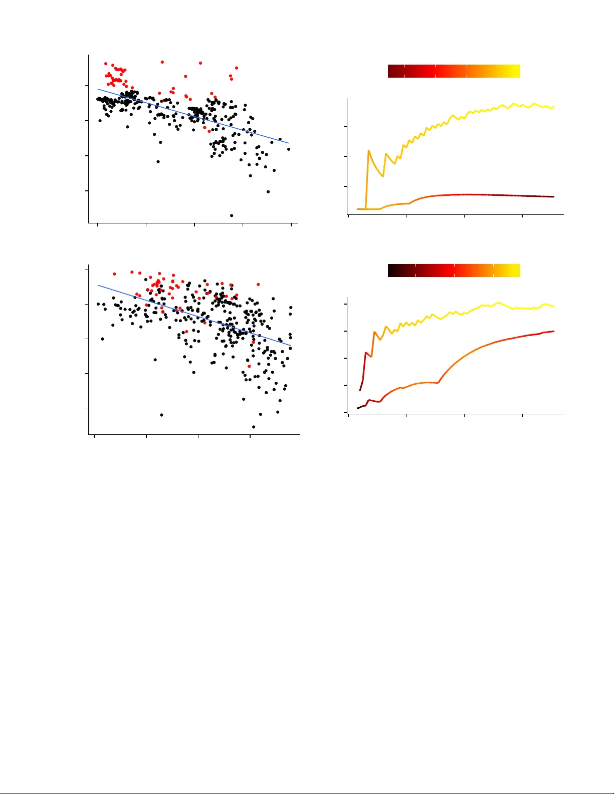
A Comparati v e Analysis of Ensemble Classifiers: Case Studies in Genomics Sean Whalen and Gaurav P andey Department of Genetics and Genomic Sciences Icahn Institute for Genomics and Multiscale Biology Icahn School of Medicine at Mount Sinai, New Y ork, USA { sean.whalen,gaurav .pandey } @mssm.edu Abstract —The combination of multiple classifiers using ensem- ble methods is increasingly important f or making progr ess in a variety of difficult pr ediction pr oblems. W e present a comparative analysis of several ensemble methods through two case studies in genomics, namely the prediction of genetic interactions and protein functions, to demonstrate their efficacy on real-w orld datasets and draw useful conclusions about their behavior . These methods include simple aggregation, meta-learning, cluster -based meta-learning, and ensemble selection using heterogeneous clas- sifiers trained on resampled data to improv e the diversity of their predictions. W e present a detailed analysis of these methods across 4 genomics datasets and find the best of these methods offer statistically significant improvements over the state of the art in their respectiv e domains. In addition, we establish a novel connection between ensemble selection and meta-learning, demonstrating how both of these disparate methods establish a balance between ensemble diversity and performance. Index T erms —Bioinformatics; Genomics; Supervised learning; Ensemble methods; Stacking; Ensemble selection I . I N T RO D U C T I O N Ensemble methods combining the output of indi vidual clas- sifiers [1], [2] hav e been immensely successful in producing accurate predictions for many comple x classification tasks [3]– [9]. The success of these methods is attributed to their ability to both consolidate accurate predictions and correct errors across many diverse base classifiers [10]. Div ersity is ke y to ensemble performance: If there is complete consensus the ensemble cannot outperform the best base classifier , yet an ensemble lacking any consensus is unlikely to perform well due to weak base classifiers. Successful ensemble methods establish a balance between the div ersity and accuracy of the ensemble [11], [12]. Howe ver , it remains largely unknown how different ensemble methods achie ve this balance to extract the maximum information from the av ailable pool of base classifiers [11], [13]. A better understanding of how different ensemble methods utilize div ersity to increase accuracy using complex datasets is needed, which we attempt to address with this paper . Popular methods like bagging [14] and boosting [15] gener- ate div ersity by sampling from or assigning weights to training examples but generally utilize a single type of base classifier to build the ensemble. Howe ver , such homogeneous ensembles may not be the best choice for problems where the ideal base classifier is unclear . One may instead build an ensemble from the predictions of a wide variety of heter ogeneous base clas- sifiers such as support vector machines, neural networks, and decision trees. T wo popular heterogeneous ensemble methods include a form of meta-learning called stacking [16], [17] as well as ensemble selection [18], [19]. Stacking constructs a higher-le vel predictiv e model over the predictions of base clas- sifiers, while ensemble selection uses an incremental strategy to select base predictors for the ensemble while balancing div ersity and performance. Due to their ability to utilize heterogeneous base classifiers, these approaches ha ve superior performance across sev eral application domains [6], [20]. Computational genomics is one such domain where classi- fication problems are especially difficult. This is due in part to incomplete kno wledge of how the cellular phenomenon of interest is influenced by the variables and measurements used for prediction, as well as a lack of consensus regarding the best classifier for specific problems. Even from a data perspectiv e, the frequent presence of extreme class imbalance, missing values, heterogeneous data sources of different scale, ov erlapping feature distributions, and measurement noise fur- ther complicate classification. These difficulties suggest that heterogeneous ensembles constructed from a large and di verse set of base classifiers, each contrib uting to the final predictions, are ideally suited for this domain. Thus, in this paper we use real-world genomic datasets (detailed in Section II-A) to analyze and compare the performance of ensemble methods for two important problems in this area: 1) prediction of pro- tein functions [21], and 2) predicting genetic interactions [9], both using high-throughput genomic datasets. Constructing accurate predictive models for these problems is notoriously difficult for the abov e reasons, and e ven small impro vements in predictiv e accuracy ha ve the potential for lar ge contrib utions to biomedical knowledge. Indeed, such improvements uncovered the functions of mitochondrial proteins [22] and sev eral other critical protein families. Similarly , the computational discovery of genetic interactions between the human genes EGFR-IFIH1 and FKBP9L-MOSC2 potentially enables novel therapies for glioblastoma [23], the most aggressive type of brain tumor in humans. W orking with important problems in computational ge- nomics, we present a comparativ e analysis of several methods used to construct ensembles from large and diverse sets of base classifiers. Sev eral aspects of heterogeneous ensemble T ABLE I D E T A I L S O F G E N E TI C I NT E R AC T IO N ( G I) A N D P ROT E I N F U N CT I O N ( P F ) DAT A S E T S I N CL U D I NG T H E N U MB E R O F F E A T U RE S , N U M B ER O F E X AM P L E S I N T H E M I N O RI T Y ( P O S IT I V E ) A N D M A J O RI T Y ( N E GAT IV E ) C L AS S E S , A N D T OTA L N U M B ER O F E X A M PL E S . Problem Features Positiv es Negati ves T otal GI 152 9,994 125,509 135,503 PF1 300 382 3,597 3,979 PF2 300 344 3,635 3,979 PF3 300 327 3,652 3,979 construction that ha ve not previously been addressed are examined in detail including a novel connection between ensemble selection and meta-learning, the optimization of the di versity/accurac y tradeoff made by these disparate ap- proaches, and the role of calibration in their performance. This analysis sheds light on ho w variants of simple greedy ensemble selection achieve enhanced performance, why meta-learning often out-performs ensemble selection, and several directions for future work. The insights obtained from the performance and behavior of ensemble methods for these complex domain- driv en classification problems should hav e wide applicability across div erse applications of ensemble learning. W e begin by detailing our datasets, experimental method- ology , and the ensemble methods studied (namely ensemble selection and stacking) in Section II. This is followed by a discussion of their performance in terms of standard e valuation metrics in Section III. W e next examine ho w the roles of div ersity and accuracy are balanced in ensemble selection and establish a connection with stacking by examining the weights assigned to base classifiers by both methods (Section IV -A). In Section IV -B, we discuss the impact of classifier calibration on heterogeneous ensemble performance, an important issue that has only recently receiv ed attention [24]. W e conclude and indicate directions for future work in Section V. I I . M AT E R I A LS A N D M E T H O D S A. Pr oblem Definitions and Datasets For this study we focus on two important problems in computational genomics: The prediction of protein functions, and the prediction of genetic interactions. Belo w we describe these problems and the datasets used to assess the efficacy of various ensemble methods. A summary of these datasets is giv en in T able I. 1) Pr otein Function Prediction: A key goal in molecular biology is to infer the cellular functions of proteins. T o keep pace with the rapid identification of proteins due to adv ances in genome sequencing technology , a large number of computa- tional approaches hav e been dev eloped to predict various types of protein functions. These approaches use various genomic datasets to characterize the cellular functions of proteins or their corresponding genes [21]. Protein function prediction is essentially a classification problem using features defined for each gene or its resulting protein to predict whether the protein performs a certain function ( 1 ) or not ( 0 ). W e use the gene expression compendium of Hughes et al. [25] to predict the T ABLE II F E A T U R E M ATR I X O F G EN E T I C I N TE R AC T I ON S W H ER E n RO W S R E PR E S E NT PAI R S O F G E NE S M EA S U R ED B Y F E A T UR E S F 1 . . . F m H A V I NG L A BE L 1 I F T HE Y A R E K N OW N T O I N T E RA CT , 0 I F T HE Y D O N OT , A N D ? I F T H EI R I NT E R AC T IO N H A S N OT B EE N E S T A B L I SH E D . Gene Pair F 1 F 2 · · · F m Interaction? Pair 1 0.5 0.1 · · · 0.7 1 Pair 2 0.2 0.7 · · · 0.8 0 . . . . . . . . . . . . . . . . . . Pair n 0.3 0.9 · · · 0.1 ? functions of roughly 4,000 baker’ s yeast ( S. cer evisiae ) genes. The three most abundant functional labels from the list of Gene Ontology Biological Process terms compiled by Myers et al. [26] are used in our e v aluation. The three corresponding prediction problems are referred to as PF1, PF2, and PF3 respectiv ely and are suitable targets for classification case studies due to their difficulty . These datasets are publicly av ailable from Pandey et al. [27]. 2) Genetic Interaction Pr ediction: Genetic interactions (GIs) are a category of cellular interactions that are inferred by comparing the effect of the simultaneous knockout of two genes with the effect of knocking them out individually [28]. The knowledge of these interactions is critical for under- standing cellular pathways [29], ev olution [30], and numerous other biological processes. Despite their utility , a general paucity of GI data exists for sev eral organisms important for biomedical research. T o address this problem, Pandey et al. [9] used ensemble classification methods to predict GIs between genes from S. cer evisiae (baker’ s yeast) using functional relationships between gene pairs such as correlation between expression profiles, extent of co-ev olution, and the presence or absence of physical interactions between their corresponding proteins. W e use the data from this study to assess the ef ficacy of heterogeneous ensemble methods for predicting GIs from a set of 152 features (see T able II for an illustration) and measure the improvement of our ensemble methods ov er this state-of-the-art. B. Experimental Setup A total of 27 heterogeneous classifier types are trained using the statistical language R [31] in combination with its various machine learning packages, as well as the R W eka interface [32] to the data mining software W eka [33] (see T able III). Among these are classifiers based on boosting and bagging which are themselves a type of ensemble method, but whose performance can be further improved by inclusion in a heterogeneous ensemble. Classifiers are trained using 10-fold cross-validation where each training split is resampled with replacement 10 times then balanced using undersampling of the majority class. The latter is a standard and essential step to pre vent learning decision boundaries biased to the majority class in the presence of extreme class imbalance such as ours (see T able I). In addition, a 5-fold nested cross-validation is performed on each training split to create a validation set for T ABLE III I N DI V I D UA L P E RF O R M AN C E O F 2 7 B A SE C L A SS I FI ER S O N G E N ET I C I N TE R AC T I ON A N D P ROT E I N F U N CT I O N DAT A S ET S E V A L UA T E D U S I N G A C O MB I NATI O N O F R [ 3 1 ] , C A R E T [ 3 4] , A N D T H E RW E K A I N T ER FAC E [ 3 2 ] T O W E K A [ 3 3 ]. D E T A I LS O F E AC H C LA S S I FIE R A R E O M I T TE D F O R B R EV I T Y . R PAC KA G ES I N CL U D E A C I T AT IO N D ES C R I BI N G T H E M E T H OD . F O R A L L O T HE R S , S E E T H E W E KA D O C UM E N T A T I O N . F O R B O O S TI N G M E TH O D S W I T H S E L E CTA B LE BA S E L E A R NE R S , T H E D E FAULT ( N O R MA L LY A D E C I SI O N S T U M P ) I S U S E D . Performance Classifier GI PF1 PF2 PF3 Functions glmboost [35] 0.72 0.65 0.71 0.72 glmnet [36] 0.73 0.63 0.71 0.73 Logistic 0.73 0.61 0.66 0.71 MultilayerPerceptron 0.74 0.64 0.71 0.74 multinom [37] 0.73 0.61 0.67 0.71 RBFClassifier 0.73 0.62 0.69 0.74 RBFNetwork 0.56 0.51 0.52 0.58 SGD 0.73 0.63 0.70 0.73 SimpleLogistic 0.73 0.65 0.72 0.73 SMO 0.73 0.64 0.70 0.73 SPegasos 0.66 0.52 0.56 0.56 V otedPerceptron 0.65 0.62 0.70 0.71 T rees AdaBoostM1 0.71 0.65 0.67 0.73 ADT ree 0.73 0.64 0.67 0.75 gbm [38] 0.77 0.68 0.72 0.78 J48 0.75 0.60 0.65 0.71 LADT ree 0.74 0.64 0.69 0.75 LMT 0.76 0.62 0.71 0.75 LogitBoost 0.73 0.65 0.69 0.75 MultiBoostAB 0.70 0.63 0.66 0.70 RandomT ree 0.71 0.57 0.60 0.63 rf [39] 0.79 0.67 0.72 0.76 Rule-Based JRip 0.76 0.63 0.67 0.70 P AR T 0.76 0.59 0.65 0.73 Other IBk 0.70 0.61 0.66 0.70 pam [40] 0.71 0.62 0.66 0.64 VFI 0.64 0.55 0.56 0.63 the corresponding test split. This validation set is used for the meta-learning and ensemble selection techniques described in Section II-C. The final result is a pool of 270 classifiers. Performance is measured by combining the predictions made on each test split resulting from cross-validation into a single set and calculating the area under the Receiv er Oper- ating Characteristic curve (A UC). The performance of the 27 base classifiers for each dataset is giv en in T able III, where the bagged predictions for each base classifier are av eraged before calculating the A UC. These numbers become important in later discussions since ensemble methods in volve a tradeoff between the div ersity of predictions and the performance of base classifiers constituting the ensemble. C. Ensemble Methods 1) Simple Aggre gation: The predictions of each base clas- sifier become columns in a matrix where rows are instances and the entry at row i , column j is the probability of instance i belonging to the positive class as as predicted by classifier j . W e ev aluate ensembles using A UC by applying the mean across rows to produce an aggregate prediction for each instance. 2) Meta-Learning: Meta-learning is a general technique for improving the performance of multiple classifiers by using the meta information they provide. A common approach to meta- learning is stacked generalization ( stacking ) [17] that trains a higher-le vel ( level 1 ) classifier on the outputs of base ( level 0 ) classifiers. Using the standard formulation of Ting and W itten [41], we perform meta-learning using stacking with a level 1 lo- gistic regression classifier trained on the pr obabilistic outputs of multiple heterogeneous lev el 0 classifiers. Though other classifiers may be used, a simple logistic regression meta- classifier helps avoid ov erfitting which typically results in superior performance [41]. In addition, its coefficients hav e an intuitive interpretation as the weighted importance of each lev el 0 classifier [6]. The layer 1 classifier is trained on a validation set created by the nested cross-validation of a particular training split and ev aluated against the corresponding test split to prev ent the leaking of label information. Ov erall performance is ev aluated as described in Section II-B. In addition to stacking across all classifier outputs, we also e valuate stacking using only the aggr e gate output of each resampled (bagged) base classifier . For example, the outputs of all 10 SVM classifiers are av eraged and used as a single level 0 input to the meta learner . Intuitiv ely this combines classifier outputs that hav e similar performance and calibration, which allo ws stacking to focus on weights between (instead of within) classifier types. 3) Cluster-Based Meta-Learning: A variant on traditional stacking is to first cluster classifiers with similar predictions, then learn a separate le vel 1 classifier for each cluster [6]. Alternately , classifiers within a cluster can first be combined by taking their mean (for example) and then learning a lev el 1 classifier on these per-cluster av eraged outputs. This is a generalization of the aggregation approach described in Section II-C2 but using a distance measure instead of restricting each cluster to bagged homogeneous classifiers. W e use hierarchical clustering with 1 − | ρ | (where ρ is Pearson’ s correlation) as a distance measure. W e found little difference between alternate distance measures based on Pearson and Spearman correlation and so present results using only this formulation. For simplicity , we refer to the method of stacking within clusters and taking the mean of le vel 1 outputs as intra-cluster stacking . Its complement, inter-cluster stacking , averages the outputs of classifiers within a cluster then performs stacking on the averaged lev el 0 outputs. The intuition for both approaches is to group classifiers with similar (but ideally non-identical) predictions together and learn how to best resolve their dis- agreements via weighting. Thus the div ersity of classifier predictions within a cluster is important, and the effecti veness of this method is tied to a distance measure that can utilize both accuracy and div ersity . 4) Ensemble Selection: Ensemble selection is the pro- cess of choosing a subset of all available classifiers that perform well together , since including every classifier may decrease performance. T esting all possible classifier com- binations quickly becomes infeasible for ensembles of any practical size and so heuristics are used to approximate the optimal subset. The performance of the ensemble can only improv e upon that of the best base classifier if the ensem- ble has a sufficient pool of accurate and div erse classifiers, and so successful selection methods must balance these two requirements. W e establish a baseline for this approach by performing simple greedy ensemble selection, sorting base classifiers by their individual performance and iterativ ely adding the best unselected classifier to the ensemble. This approach disregards how well the classifier actually complements the performance of the ensemble. Improving on this approach, Caruana et al. ’ s ensemble selection (CES) [18], [19] begins with an empty ensemble and iterativ ely adds ne w predictors that maximize its performance according to a chosen metric (here, A UC). At each iteration, a number of candidate classifiers are randomly selected and the performance of the current ensemble including the candidate is e v aluated. The candidate resulting in the best ensemble performance is selected and the process repeats until a maxi- mum ensemble size is reached. The ev aluation of candidates according to their performance with the ensemble, instead of in isolation, improves the performance of CES over simple greedy selection. Additional improvements over simple greedy selection in- clude 1) initializing the ensemble with the top n base clas- sifiers, and 2) allowing classifiers to be added multiple times. The latter is particularly important as without replacement, the best classifiers are added early and ensemble performance then decreases as poor predictors are forced into the ensem- ble. Replacement giv es more weight to the best performing predictors while still allowing for div ersity . W e use an initial ensemble size of n = 2 to reduce the effect of multiple bagged versions of a single high performance classifier dominating the selection process, and (for completeness) ev aluate all candidate classifiers instead of sampling. Ensemble predictions are combined using a cumulativ e moving average to speed the ev aluation of ensemble perfor- mance for each candidate predictor . Selection is performed on the validation set produced by nested cross-validation and the resulting ensemble ev aluated as described in Section II-B. D. Diversity Measures The div ersity of predictions made by members of an en- semble determines the ensemble’ s ability to outperform the best indi vidual, a long-accepted property which we explore in the following sections. W e measure div ersity using Y ule’ s Q - statistic [42] by first creating predicted labels from thresholded classifier probabilities, yielding a 1 for values greater than 0.5 and 0 otherwise. Giv en the predicted labels produced by each pair of classifiers D i and D k , we generate a contingenc y table counting ho w often each classifier produces the correct label in relation to the other: D k correct (1) D k incorrect (0) D i correct (1) N 11 N 10 D i wrong (0) N 01 N 00 The pairwise Q statistic is then defined as: Q i,k = N 11 N 00 − N 01 N 10 N 11 N 00 + N 01 N 10 . (1) This produces values tending towards 1 when D i and D k correctly classify the same instances, 0 when they do not, and − 1 when they are negativ ely correlated. W e ev aluated additional di versity measures such as Cohen’ s κ -statistic [43] but found little practical dif ference between the measures (in agreement with Kunche v a et al. [11]) and focus on Q for its simplicity . Multicore performance and diversity measures are implemented in C++ using the Rcpp package [44]. This prov es essential for their practical use with large ensembles and nested cross validation. W e adjust raw Q values using the transformation 1 − | Q | so that 0 represents no div ersity and 1 represents maximum div ersity for graphical clarity . I I I . E N S E M B L E P E R F O R M A N C E Performance of the methods described in Section II-C is summarized in T able IV. Overall, aggregated stacking is the best performer and edges out CES for all our datasets. The use of clustering in combination with stacking also performs well for certain cluster sizes k . Intra-cluster stacking performs best with cluster sizes 2, 14, 20, and 15 for GI, PF1, PF2, and PF3, respectiv ely . Inter-cluster stacking is optimal for sizes 24, 33, 33, and 36 on the same datasets. Due to the size of the GI dataset, only 10% of the validation set is used for non-aggreg ate stacking and cluster stacking methods. Performance lev els off beyond 10% and so this approach does not significantly penalize these methods. This step was not necessary for the other methods and datasets. Ensemble selection also performs well, though we anticipate issues of calibration (detailed in Section IV -B) could hav e a negati ve impact since the mean is used to aggreg ate ensemble predictions. Greedy selection achieves best performance for ensemble sizes of 10, 14, 45, and 38 for GI, PF1, PF2, and PF3, respecti vely . CES is optimal for sizes 70, 43, 34, and 56 for the same datasets. Though the best performing ensembles for both selection methods are close in performance, simple greedy selection is much worse for non-optimal ensemble sizes than CES and its performance typically degrades after the best few base classifiers are selected (see Section IV -A). Thus, on av erage CES is the superior selection method. In agreement with Altman et al. [6], we find the mean is the highest performing simple aggregation method for combining ensemble predictions. Howe ver , because we are using heterogeneous classifiers that may hav e uncalibrated outputs, the mean combines predictions made with different T ABLE IV AU C O F E N S EM B L E L E A RN I N G M E T HO D S F O R P RO TE I N F U N C TI O N A N D G E NE T I C I N T ER AC T I O N D A TA SE T S . M E T HO D S I N C L UD E M EA N AG G R EG ATI O N , G R E EDY E N S EM B L E S E LE C T I ON , S E LE C T IO N W I TH R E PL AC E M E NT ( C E S) , S T A C KI N G W I T H L O GI S T I C R E GR E S S IO N , AG G R EG ATE D S T AC K I NG ( A V E RA G IN G R ES A M P LE D H O MO G E NE O U S B AS E C L AS S I FI ER S B E F O RE S TAC KI N G ) , S TAC K IN G W I TH I N C L U S TE R S T H E N A V E R AG IN G ( I NT R A ) , A N D A V E RA GI N G W I T H IN C L US T E R S T H EN S T AC K I NG ( I N TR A ) . T H E B E S T P E R FO R M I NG BA S E C L A S SI FI E R ( R A ND O M F O RE S T F O R T H E G I DAT A S E T A N D G B M F O R P F S ) I S G IV E N F O R R E FE R E N CE . S T A R R E D V A L U ES A R E G E N ER A T E D F RO M A S U BS A M P LE O F T H E VAL I DATI O N S E T D U E T O I T S S I Z E ; S E E T E X T F O R D E TAI L . Performance Method GI PF1 PF2 PF3 Best Base Classifier 0.79 0.68 0.72 0.78 Mean Aggregation 0.763 0.669 0.732 0.773 Greedy Selection 0.792 0.684 0.734 0.779 CES 0.802 0.686 0.741 0.785 Stacking (Aggregated) 0.812 0.687 0.742 0.788 Stacking (All) 0.809 ∗ 0.684 0.726 0.773 Intra-Cluster Stacking 0.799 ∗ 0.684 0.725 0.775 Inter-Cluster Stacking 0.786 ∗ 0.683 0.735 0.783 T ABLE V P A I RW IS E P E R F OR M A N CE C O M P A R I SO N O F M U L T I PL E N ON - E N SE M B L E A N D E N SE M B L E M E T H OD S AC RO S S D A TAS E T S . O N LY PA I RS W I T H S T A T IS T I C AL LY S I GN I FI C AN T D I FFE R E NC E S , D E T ER M I N ED B Y F R IE D M A N / N E M EN Y I T E S TS AT α = 0 . 05 , A R E S H OW N . Method A Method B p-value Best Base Classifier CES 0.001902 Best Base Classifier Stacking (Aggregated) 0.000136 CES Inter-Cluster Stacking 0.037740 CES Intra-Cluster Stacking 0.014612 CES Mean Aggregation 0.000300 CES Stacking (All) 0.029952 Greedy Selection Mean Aggregation 0.029952 Greedy Selection Stacking (Aggregated) 0.005364 Inter-Cluster Stacking Mean Aggregation 0.047336 Inter-Cluster Stacking Stacking (Aggregated) 0.003206 Intra-Cluster Stacking Stacking (Aggregated) 0.001124 Mean Aggregation Stacking (Aggregated) 0.000022 Stacking (Aggregated) Stacking (All) 0.002472 T ABLE VI G RO U PE D P E RF O R M AN C E C O M P A R I S ON O F M U LTI P L E N O N - E N S EM B L E A N D E N SE M B L E M E T H OD S AC RO S S D A TAS E T S . M E T H OD S S H AR I N G A G RO U P L E TT E R H A V E S T A T IS T I C AL LY S I MI L A R P E R FO R M A NC E , D E TE R M I NE D B Y F RI E D M AN / N E ME N Y I T E ST S A T α = 0 . 05 . A GG R E G A T E D S T AC K I NG A N D C E S D E M ON S T RAT E T H E B E ST P E RF O R M AN C E , W H I LE G R EE DY S E LE C T I ON I S S I M IL A R T O C E S ( B U T N OT S T A C KI N G ) . Group Method Rank Sum a Stacking (Aggregated) 32 ab CES 27 bc Greedy Selection 18 c Inter-Cluster Stacking 17 cd Stacking (All) 16.5 cd Intra-Cluster Stacking 15 cd Best Base Classifier 11 d Mean Aggregation 7.5 scales or notions of probability . This explains its poor perfor- mance compared to the best base classifier in a heterogeneous ensemble and emphasizes the need for ensemble selection or weighting via stacking to take full adv antage of the ensemble. W e discuss the issue of calibration in Section IV -B. Thus, we observe consistent performance trends across these methods. Ho wev er, to draw meaningful conclusions it is criti- cal to determine if the performance differences are statistically significant. For this we employ the standard methodology giv en by Dem ˇ sar [45] to test for statistically significant perfor- mance dif ferences between multiple methods across multiple datasets. The Friedman test [46] first determines if there are statistically significant differences between any pair of methods over all datasets, followed by a post-hoc Nemenyi test [47] to calculate a p-value for each pair of methods. This is the non-parametric equiv alent of ANO V A combined with a T ukey HSD post-hoc test where the assumption of normally distributed v alues is remov ed by using rank transformations. As many of the assumptions of parametric tests are violated by machine learning algorithms, the Friedman/Nemenyi test is preferred despite reduced statistical power [45]. Using the Freidman/Nemeyi approach with a cutoff of α = 0 . 05 , the pairwise comparison between our ensemble and non-ensemble methods is shown in T able V. For brevity , only methods with statistically significant performance differ - ences are shown. The ranked performance of each method across all datasets is shown in T able VI. Methods sharing a label in the group column have statistically indistinguishable performance based on their summed rankings. This table shows that aggregated stacking and CES have the best perfor- mance, while CES and pure greedy selection have similar per - formance. Howe ver , aggregated stacking and greedy selection do not share a group as their summed ranks are too distant and thus have a significant performance dif ference. The remaining approaches including non-aggregated stacking are statistically similar to mean aggregation and motiv ates our inclusion of cluster-based stacking, whose performance may improve gi ven a more suitable distance metric. These rankings statistically reinforce the general trends presented earlier in T able IV. W e note that nested cross-validation, relative to a single validation set, improv es the performance of both stacking and CES by increasing the amount of meta data av ailable as well as the bagging that occurs as a result. Both effects reduce ov erfitting but performance is still typically better with smaller ensembles. More nested folds increase the quality of the meta data and thus af fects the performance of these methods as well, though computation time increases substantially and motiv ates our selection of k = 5 nested folds. Finally , we emphasize that each method we ev aluate out- performs the previous state of the art A UC of 0.741 for GI prediction [9]. In particular , stacked aggregation results in the prediction of 988 additional genetic interactions at a 10% false discovery rate. In addition, these heterogeneous ensemble methods out-perform random forests and gradient boosted regression models which are themselv es homogeneous ensembles. This demonstrates the value of heterogeneous 0.60 0.65 0.70 0.75 0.00 0.25 0.50 0.75 1.00 P airwise Div ersity (1 − |Q|) P airwise P erformance (A UC) 0.55 0.60 0.65 0.70 0.75 0.00 0.25 0.50 0.75 P airwise Div ersity (1 − |Q|) P airwise P erformance (A UC) Fig. 1. Performance as a function of diversity for all pairwise combinations of 27 base classifiers on the GI (top figure) and PF3 (bottom figure) datasets. More div erse combinations typically result in less performance except for high-performance classifiers such as random forests and generalized boosted regression models, whose points are shown in red if they are part of a pair . Raw Q values are adjusted so that larger values imply more div ersity . ensembles for improving predictiv e performance. I V . E N S E M B L E C H A R A C T E R I S T I C S A. The Role of Diversity The relationship between ensemble div ersity and perfor- mance has immediate impact on practitioners of ensemble methods, yet has not formally been proven despite extensiv e study [11], [13]. For brevity we analyze this tradeoff using GI and PF3 as representativ e datasets, though the trends observed generalize to PF1 and PF2. Figure 1 presents a high-le vel view of the relationship between performance and div ersity , plotting the div ersity of pairwise classifiers against their performance as an ensemble by taking the mean of their predictions. This figure shows the 0.1 0.2 0.3 0 20 40 60 Iteration Ensem ble Div ersity (1 − |Q|) .76 .77 .78 .79 Ensem ble P erformance (A UC) 0.1 0.2 0.3 0.4 0.5 0 20 40 60 Iteration Ensem ble Div ersity (1 − |Q|) .76 .77 .78 Ensem ble P erformance (A UC) Fig. 2. Ensemble div ersity and performance as a function of iteration number for both greedy selection (bottom curve) and CES (top curve) on the GI and PF3 datasets. For GI (top figure), greedy selection fails to improve diversity and performance decreases with ensemble size, while CES successfully balances diversity and performance (shown by a shift in color from red to yellow as height increases) and reaches an equilibrium over time. For PF3 (bottom figure), greedy selection manages to improve di versity around iteration 30 but accuracy decreases, demonstrating that di verse predictions alone are not enough for accurate ensembles. complicated relationship between div ersity and performance that holds for each of our datasets: T wo highly div erse classifiers are more likely to perform poorly due to lower prediction consensus. There are exceptions, and these tend to include well-performing base classifiers such as random forests and gradient boosted regression models (shown in red in Figure 1) which achiev e high A UC on their o wn and stand to gain from a div erse partner . Div ersity works in tension with performance, and while improving performance depends on div ersity , the wrong kind of div ersity limits performance of the ensemble [48]. Figure 2 demonstrates this tradeoff by plotting ensemble div ersity and performance as a function of the iteration number of the simple greedy selection and CES methods detailed in T ABLE VII T H E M O ST - WE I G H TE D C L AS S I FIE R S P RO D U C ED B Y S TAC K IN G W I TH L O GI S T I C R E G R ES S I O N ( W E I GH T m ) A N D C E S ( W E I GH T c ) F O R T H E P F 3 DAT A S E T , A L O N G W I T H T H E IR A V E R AG E PA IR WI S E D I V ER S I T Y A N D P E RF O R M AN C E . Classifier W eight m W eight c Div . A UC rf 0.25 0.21 0.39 0.71 gbm 0.20 0.27 0.42 0.72 RBFClassifier - 0.05 0.45 0.71 MultilayerPerceptron 0.09 - 0.46 0.70 SGD 0.09 0.04 0.47 0.69 VFI 0.11 0.11 0.71 0.66 IBk 0.09 0.13 0.72 0.68 Section II for the GI (top figure) and PF3 (bottom figure) datasets. These figures rev eal how CES (top curve) success- fully exploits the tradeoff between di versity and performance while a purely greedy approach (bottom curve) actually de- creases in performance over iterations after the best individual base classifiers are added. This is shown via coloring, where CES shifts from red to yellow (better performance) as its div ersity increases while greedy selection grows darker red (worse performance) as its diversity only slightly increases. Note that while greedy selection increases ensemble diversity around iteration 30 for PF3, ov erall performance continues to decrease. This demonstrates that div ersity must be balanced with accuracy to create well-performing ensembles. T o illustrate using the PF3 panel of Figure 2, the first classi- fiers chosen by CES (in order) are rf.1, rf.7, gbm.2, RBFClas- sifier .0, MultilayerPerceptron.9, and gbm.3 where numbers indicate bagged versions of a base classifier . RBFClassifier .0 is a lo w performance, high div ersity classifier while the others are the opposite (see T able III for a summary of base classifiers). This ensemble shows ho w CES tends to repeatedly select base classifiers that improve performance, then selects a more div erse and typically worse performing classifier . Here the former are different bagged versions of a random forest while the latter is RBFClassifier .0. This manifests in the left part of the upper curve where diversity is low and then jumps to its first peak. After this, a random forest is added again to balance performance and di versity drops until the next peak. This process is repeated while the algorithm approaches a weighted equilibrium of high performing, low diversity and low performing, high div ersity classifiers. This agrees with recent observations that di versity enforces a kind of regularization for ensembles [13], [49]: Performance stops increasing when there is no more div ersity to extract from the pool of possible classifiers. W e see this in the PF3 panel of Figure 2 as performance reaches its peak, where small oscillations in diversity represent re-balancing the weights to maintain performance past the optimal ensemble size. Since ensemble selection and stacking are top performers and can both be interpreted as learning to weight different base classifiers, we next compare the most heavily weighted classifiers selected by CES (W eight c ) with the coefficients of a lev el 1 logistic regression meta-learner (W eight m ). W e com- T ABLE VIII C A ND I DATE C L A SS I FI ER S S O RTE D B Y M E AN PA IR WI S E D I V ER S I T Y A N D P E RF O R M AN C E . T H E M O S T H E A V I L Y W E I GH T E D C L AS S I FI ER S F OR B OT H C E S A N D S TAC K IN G A R E S H OW N I N B O L D . T H IS T R E ND , W HI C H H O L D S AC RO S S D A TA SE T S , S H OW S T H E PA IR I N G O F H I G H - P E R F OR M A N CE L OW - D IV E R S IT Y C LA S S I FIE R S W I T H T H E IR C O MP L E M EN T S , D E MO N S T RATI N G H O W S E EM I N G L Y D I SPA R A T E A P P ROA CH E S C R E A T E A BA L A N CE O F D I V ER S I T Y A N D P E R F OR M A N CE . Classifier Div ersity A UC rf 0.386 0.712 gbm 0.419 0.720 glmnet 0.450 0.694 glmboost 0.452 0.680 RBFClassifier 0.453 0.713 SimpleLogistic 0.459 0.689 MultilayerPer ceptron 0.459 0.706 SMO 0.462 0.695 SGD 0.470 0.693 LMT 0.472 0.692 pam 0.525 0.673 LogitBoost 0.528 0.691 ADT ree 0.539 0.682 V otedPerceptron 0.540 0.694 multinom 0.553 0.677 LADT ree 0.568 0.678 Logistic 0.574 0.669 AdaBoostM1 0.584 0.684 P AR T 0.615 0.652 MultiBoostAB 0.615 0.679 J48 0.632 0.645 JRip 0.687 0.627 VFI 0.713 0.662 IBk 0.720 0.682 RBFNetwork 0.778 0.653 RandomT ree 0.863 0.602 SPegasos 0.980 0.634 pute W eight c as the normalized counts of classifiers included in the ensemble, resulting in greater weight for classifiers selected multiple times. These weights for PF3 are shown in T able VII. Nearly the same classifiers receive the most weight under both approaches (though logistic regression coefficients were not restricted to positiv e v alues so we cannot directly compare weights between methods). Howe ver , the general trend of the relativ e weights is clear and explains the oscillations seen in Figure 2: High performance, lo w di versity classifiers are repeatedly paired with higher di versity , lower performing classifiers. A more complete picture of selection emerges by examining the full list of candidate base classifiers (T able VIII) with the most weighted ensemble classifiers shown in bold. The highest performing, lowest div ersity GBM and RF classi- fiers appear at the top of the list while VFI and IBk are near the bottom. Though there are more di verse classifiers than VFI and IBk, they were not selected due to their lower performance. This example illustrates how diversity and performance are balanced during selection, and also gi ves new insight into the nature of stacking due to the con vergent weights of these seemingly dif ferent approaches. A metric incorporating both measures should increase the performance of hybrid methods such as cluster-based stacking, which we plan to in vestigate in future work. Base Classifiers Ensembles (CES) Ensembles (Greedy) 0.6 0.7 0.7875 0.7900 0.7925 0.7950 0.76 0.77 0.78 0.1 0.2 0.3 0.140 0.145 0.150 0.155 0.15 0.16 0.17 0.18 Brier Score P erformance (A UC) Fig. 3. Performance as a function of calibration as measured by the Brier score [50] for base classifiers (left), ensembles for each iteration of CES (middle), and ensembles for each strictly greedy iteration (right). Iterations for greedy selection move from the upper left to the lo wer right, while CES starts in the lower right and moves to the upper left. This shows better-calibrated (lower Brier score) classifiers and ensembles have higher average performance and illustrates the iterative performance differences between the methods. Stacking with logistic regression produces outputs with approximately half the best Brier score of CES, explaining the difference in final classifier weights leading to the superior performance of stacking. B. The Role of Calibration A ke y factor in the performance dif ference between stacking and CES is illustrated by stacking’ s selection of Multilayer- Perceptron instead of RBFClassifier for PF3. This difference in the relative weighting of classifiers, or the exchange of one classifier for another in the final ensemble, persists across our datasets. W e suggest this is due to the ability of the layer 1 classifier to learn a function on the probabilistic outputs of base classifiers and compensate for potential differences in calibration , resulting in the superior performance of stacking. A binary classifier is said to be well-calibrated if it is cor- rect p percent of the time for predictions of confidence p [24]. Howe ver , accuracy and calibration are related b ut not the same: A binary classifier that flips a fair coin for a balanced dataset will be calibrated but not accurate. Relatedly , many well- performing classifiers do not produce calibrated probabilities. Measures such as A UC are not sensiti ve to calibration for base classifiers, and the effects of calibration on heterogeneous ensemble learning hav e only recently been studied [24]. This section further in vestigates this relationship. T o illustrate a practical example of calibration, consider a support vector machine. An uncalibrated SVM outputs the distance of an instance from a hyperplane to generate a probability . This is not a true posterior probability of an instance belonging to a class, but is commonly conv erted to such using Platt’ s method [51]. In fact, this is analogous to fitting a layer 1 logistic regression to the uncalibrated SVM outputs with a slight modification to av oid overfitting. This approach is not restricted to SVMs and additional methods such as isotonic regression are commonly used for both binary and multi-class problems [52]. Regardless of the base classifier , a lack of calibration may effect the performance of ensemble selection methods such as CES since the predictions of many heterogeneous classifiers are combined using simple aggregation methods such as the mean. Several methods exist for ev aluating the calibration of probabilistic classifiers. One such method, the Brier scor e , assesses how close (on av erage) a classifier’ s probabilistic output is to the correct binary label [50]: B S = 1 N N X i =1 ( f i − o i ) 2 (2) ov er all instances i . This is simply the mean squared error ev aluated in the context of probabilistic binary classification. Lower scores indicate better calibration. Figure 3 plots the Brier scores for each base classifier against its performance for the GI dataset as well as the ensemble Brier scores for each iteration of CES and greedy selection. This shows that classifiers and ensembles with calibrated outputs generally perform better . Note in particular the calibration and performance of simple greedy selection, with initial iterations in the upper left of the panel showing high performing well-calibrated base classifiers chosen for the ensemble, but moving to the lower right as sub-optimal classifiers are forced into the ensemble. In contrast, CES starts with points in the lo wer right and moves to the upper left as both ensemble calibration and performance improv e each iteration. The upper left of the CES plot suggests the benefit of additional classifiers outweighs a loss in calibration during its final iterations. Stacking produces a layer 1 classifier with approximately half the Brier score (0.083) of CES or the best base classifiers. Since this approach learns a function ov er probabilities it is able to adjust to the different scales used by potentially ill- calibrated classifiers in a heterogeneous ensemble. This ex- plains the difference in the final weights assigned by stacking and CES to the base classifiers in T able VII: Though the relativ e weights are mostly the same, logistic regression is able to correct for the lack of calibration across classifiers and better incorporate the predictions of MultilayerPerceptron whereas CES cannot. In this case, a calibrated MultilayerPerceptron serves to improv e performance of the ensemble and thus stacking outperforms CES. In summary , this section demonstrates the tradeof f between performance and di versity made by CES and examines its connection with stacking. There is significant ov erlap in the relativ e weights of the most important base classifiers selected by both methods. From this set of classifiers, stacking often assigns more weight to a particular classifier as compared to CES and this result holds across our datasets. W e attribute the superior performance of stacking to this dif ference, originat- ing from its ability to accommodate differences in classifier calibration that are likely to occur in large heterogeneous ensembles. This claim is substantiated by its significantly lower Brier score compared to CES as well as the correlation between ensemble calibration and performance. This suggests the potential for improving ensemble methods by accommo- dating differences in calibration. V . C O N C L U S I O N S A N D F U T U R E W O R K The aim of ensemble techniques is to combine div erse clas- sifiers in an intelligent way such that the predictiv e accuracy of the ensemble is greater than that of the best base classifier . Since enumerating the space of all classifier combinations quickly becomes infeasible for ev en relativ ely small ensemble sizes, other methods for finding well performing ensembles hav e been widely studied and applied in the last decade. In this paper we apply a variety of ensemble approaches to two difficult problems in computational genomics: The prediction of genetic interactions and the prediction of pro- tein functions. These problems are notoriously difficult for their extreme class imbalance, prev alence of missing values, integration of heterogeneous data sources of different scale, and ov erlap between feature distributions of the majority and minority classes. These issues are amplified by the inherent complexity of the underlying biological mechanisms and in- complete domain knowledge. W e find that stacking and ensemble selection approaches offer statistically significant improv ements ov er the previous state-of-the-art for GI prediction [9] and moderate improve- ments over tuned random forest classifiers which are par- ticularly effecti ve in this domain [5]. Here, even small im- prov ements in accuracy can contribute directly to biomedical knowledge after wet-lab verification: These include 988 addi- tional genetic interactions predicted by aggre gated stacking at a 10% false disco very rate. W e also uncov er a novel connection between stacking and Caruana et al. ’ s ensemble selection method (CES) [18], [19], demonstrating how these two dis- parate methods con verge to nearly the same final base classifier weights by balancing div ersity and performance in different ways. W e e xplain how v ariations in these weights are related to the calibration of base classifiers in the ensemble, and finally describe how stacking improves accuracy by accounting for differences in calibration. This connection also sho ws how the utilization of diversity is an emergent, not explicit, property of how CES maximizes ensemble performance and suggests directions for future work including formalizing the ef fects of calibration on heterogeneous ensemble performance, modifica- tions to CES which explicitly incorporate di versity [49], and an optimization-based formulation of the div ersity/performance tradeoff for improving cluster-based stacking methods. V I . A C K N OW L E D G E M E N T S W e thank the Genomics Institute at Mount Sinai for their generous financial and technical support. R E F E R E N C E S [1] L. Rokach, “Ensemble-Based Classifiers, ” Artificial Intelligence Review , vol. 33, no. 1-2, pp. 1–39, 2009. [2] G. Seni and J. Elder , Ensemble Methods in Data Mining: Impr oving Accuracy Through Combining Predictions . Morgan & Claypool, 2010. [3] J. Shotton, A. Fitzgibbon, M. Cook, T . Sharp, M. Finocchio, R. Moore, A. Kipman, and A. Blake, “Real-Time Human Pose Recognition in Parts from Single Depth Images, ” in Proceedings of the 2011 IEEE Confer ence on Computer V ision and P attern Recognition , 2011, pp. 1297–1304. [4] D. Kim, “Forecasting Time Series with Genetic Fuzzy Predictor Ensem- ble, ” IEEE T ransactions on Fuzzy Systems , vol. 5, no. 4, pp. 523–535, 1997. [5] P . Y ang, Y . H. Y ang, B. B. Zhou, and A. Y . Zomaya, “A Review of Ensemble Methods in Bioinformatics, ” Curr ent Bioinformatics , vol. 5, no. 4, pp. 296–308, 2010. [6] A. Altmann, M. Rosen-Zvi, M. Prosperi, E. Aharoni, H. Neuvirth, E. Sch ¨ ulter , J. B ¨ uch, D. Struck, Y . Peres, F . Incardona, A. S ¨ onnerborg, R. Kaiser, M. Zazzi, and T . Lengauer, “Comparison of Classifier Fusion Methods for Predicting Response to Anti HIV -1 Therapy , ” PLoS ONE , vol. 3, no. 10, p. e3470, 2008. [7] M. Liu, D. Zhang, and D. Shen, “Ensemble Sparse Classification of Alzheimer’ s Disease, ” Neuroima ge , vol. 60, no. 2, pp. 1106–1116, 2012. [8] A. Khan, A. Majid, and T .-S. Choi, “Predicting Protein Subcellular Location: Exploiting Amino Acid Based Sequence of Feature Spaces and Fusion of Di verse Classifiers, ” Amino Acids , vol. 38, no. 1, pp. 347–350, 2010. [9] G. Pandey , B. Zhang, A. N. Chang, C. L. Myers, J. Zhu, V . Kumar , and E. E. Schadt, “An Integrative Multi-Network and Multi-Classifier Approach to Predict Genetic Interactions, ” PLoS Computational Biology , vol. 6, no. 9, p. e1000928, 2010. [10] K. T umer and J. Ghosh, “Error Correlation and Error Reduction in Ensemble Classifiers, ” Connection Science , vol. 8, no. 3-4, pp. 385– 404, 1996. [11] L. I. Kunchev a and C. J. Whitaker, “Measures of Div ersity in Classi- fier Ensembles and Their Relationship with the Ensemble Accuracy , ” Machine Learning , vol. 51, no. 2, pp. 181–207, 2003. [12] T . G. Dietterich, “An Experimental Comparison of Three Methods for Constructing Ensembles of Decision Trees: Bagging, Boosting, and Randomization, ” Machine Learning , vol. 40, no. 2, pp. 139–157, 2000. [13] E. K. T ang, P . N. Suganthan, and X. Y ao, “An Analysis of Diversity Measures, ” Machine Learning , vol. 65, no. 1, pp. 247–271, 2006. [14] L. Breiman, “Bagging Predictors, ” Machine Learning , vol. 24, no. 2, pp. 123–140, 1996. [15] R. E. Schapire and Y . Freund, Boosting: F oundations and Algorithms . MIT Press, 2012. [16] C. J. Merz, “Using Correspondence Analysis to Combine Classifiers, ” Machine Learning , vol. 36, no. 1-2, pp. 33–58, 1999. [17] D. H. W olpert, “Stacked Generalization, ” Neural Networks , vol. 5, no. 2, pp. 241–259, 1992. [18] R. Caruana, A. Niculescu-Mizil, G. Crew , and A. Ksikes, “Ensemble Selection from Libraries of Models, ” in Pr oceedings of the 21st Inter- national Confer ence on Machine Learning , 2004, pp. 18–26. [19] R. Caruana, A. Munson, and A. Niculescu-Mizil, “Getting the Most Out of Ensemble Selection, ” in Proceedings of the 6th International Confer ence on Data Mining , 2006, pp. 828–833. [20] A. Niculescu-Mizil, C. Perlich, G. Swirszcz, V . Sindhwani, and Y . Liu, “W inning the KDD Cup Orange Challenge with Ensemble Selection, ” Journal of Machine Learning Resear ch Pr oceedings T rack , vol. 7, pp. 23–24, 2009. [21] G. Pandey , V . Kumar , and M. Steinbach, “Computational Approaches for Protein Function Prediction: A Survey, ” University of Minnesota, T ech. Rep., 2006. [22] D. C. Hess, C. L. Myers, C. Huttenhower , M. A. Hibbs, A. P . Hayes, J. Pa w , J. J. Clore, R. M. Mendoza, B. S. Luis, C. Nislow , G. Giaev er , M. Costanzo, O. G. Troyanskaya, and A. A. Caudy , “Computationally Driv en, Quantitativ e Experiments Discover Genes Required for Mito- chondrial Biogenesis, ” PLoS Genetics , vol. 5, no. 3, p. e1000407, 2009. [23] E. Szczurek, N. Misra, and M. V ingron, “Synthetic Sickness or Lethality Points at Candidate Combination Therapy T argets in Glioblastoma, ” International Journal of Cancer , 2013. [24] A. Bella, C. Ferri, J. Hern ´ andez-Orallo, and M. J. Ram ´ ırez-Quintana, “On the Effect of Calibration in Classifier Combination, ” Applied Intelligence , pp. 1–20, 2012. [25] T . R. Hughes, M. J. Marton, A. R. Jones, C. J. Roberts, R. Stoughton, C. D. Armour, H. A. Bennett, E. Coffey , H. Dai, Y . D. He, M. J. Kidd, A. M. King, M. R. Meyer , D. Slade, P . Y . Lum, S. B. Stepaniants, D. D. Shoemaker, D. Gachotte, K. Chakraburtty , J. Simon, M. Bard, and S. H. Friend, “Functional Discov ery via a Compendium of Expression Profiles, ” Cell , vol. 102, no. 1, pp. 109–126, 2000. [26] C. L. Myers, D. R. Barrett, M. A. Hibbs, C. Huttenhower , and O. G. T royanskaya, “Finding Function: Evaluation Methods for Functional Genomic Data, ” BMC Genomics , vol. 7, no. 187, 2006. [27] G. Pandey , C. L. Myers, and V . Kumar , “Incorporating Functional Inter-Relationships Into Protein Function Prediction Algorithms, ” BMC Bioinformatics , vol. 10, no. 142, 2009. [28] J. L. Hartman, B. Garvik, and L. Hartwell, “Principles for the Buffering of Genetic V ariation, ” Science , vol. 291, no. 5506, pp. 1001–1004, 2001. [29] T . Horn, T . Sandmann, B. Fischer , E. Axelsson, W . Huber , and M. Boutros, “Mapping of Signaling Networks Through Synthetic Ge- netic Interaction Analysis by RNAi, ” Nature Methods , vol. 8, no. 4, pp. 341–346, 2011. [30] B. V anderSluis, J. Bellay , G. Musso, M. Costanzo, B. Papp, F . J. V izeacoumar, A. Baryshnikova, B. J. Andrews, C. Boone, and C. L. Myers, “Genetic Interactions Reveal the Evolutionary Trajectories of Duplicate Genes, ” Molecular Systems Biology , vol. 6, no. 1, 2010. [31] R Core T eam, “R: A Language and Environment for Statistical Com- puting, ” 2012. [32] K. Hornik, C. Buchta, and A. Zeileis, “Open-Source Machine Learning: R Meets W eka, ” Computational Statistics , vol. 24, no. 2, pp. 225–232, 2009. [33] M. Hall, E. Frank, G. Holmes, B. Pfahringer , P . Reutemann, and I. H. W itten, “The WEKA Data Mining Software: An Update, ” SIGKDD Explorations , vol. 11, no. 1, pp. 10–18, 2009. [34] M. Kuhn, “Building Predictiv e Models in R Using the caret Package, ” Journal of Statistical Software , vol. 28, no. 5, pp. 1–26, 2008. [35] T . Hothorn, P . B ¨ uhlmann, T . Kneib, M. Schmid, and B. Hofner, “Model- Based Boosting 2.0, ” Journal of Machine Learning Resear ch , vol. 11, no. Aug, pp. 2109–2113, 2010. [36] J. H. Friedman, T . Hastie, and R. J. Tibshirani, “Regularization Paths for Generalized Linear Models via Coordinate Descent, ” Journal of Statistical Softwar e , vol. 33, no. 1, pp. 1–22, 2010. [37] W . N. V enables and B. D. Ripley , Modern Applied Statistics with S , 4th ed. Springer , 2002. [38] G. Ridgew ay , “gbm: Generalized Boosted Regression Models, ” 2013. [39] A. Liaw and M. Wiener , “Classification and Regression by randomFor- est, ” R News , vol. 2, no. 3, pp. 18–22, 2002. [40] T . Hastie, R. J. T ibshirani, B. Narasimhan, and G. Chu, “Diagnosis of Multiple Cancer T ypes by Shrunken Centroids of Gene Expression, ” Pr oceedings of the National Academy of Sciences of the United States of America , vol. 99, no. 10, pp. 6567–6572, 2002. [41] K. M. Ting and I. H. Witten, “Issues in Stacked Generalization, ” Journal of Artificial Intelligence Research , vol. 10, no. 1, pp. 271–289, 1999. [42] G. U. Y ule, “On the Association of Attributes in Statistics: With Illustrations from the Material of the Childhood Society , ” Philosophical T ransactions of the Royal Society of London, Series A , vol. 194, pp. 257–319, 1900. [43] J. Cohen, “A Coefficient of Agreement for Nominal Scales, ” Educational and Psychological Measurement , vol. 20, no. 1, pp. 37–46, 1960. [44] D. Eddelbuettel and R. Franc ¸ ois, “Rcpp: Seamless R and C++ Integra- tion, ” Journal of Statistical Software , vol. 40, no. 8, pp. 1–18, 2011. [45] J. Dem ˇ sar , “Statistical Comparisons of Classifiers ov er Multiple Data Sets, ” Journal of Machine Learning Researc h , vol. 7, no. Jan, pp. 1–30, 2006. [46] M. Friedman, “The Use of Ranks to A void the Assumption of Normality Implicit in the Analysis of V ariance, ” Journal of the American Statistical Association , vol. 32, no. 200, pp. 675–701, 1937. [47] P . B. Nemenyi, “Distribution-Free Multiple Comparisons, ” Ph.D. disser- tation, Princeton Univ ersity , 1963. [48] G. Brown and L. I. Kunchev a, ““Good” and “Bad” Diversity in Majority V ote Ensembles, ” in Pr oceedings of the 9th International Confer ence on Multiple Classifier Systems , 2010, pp. 124–133. [49] N. Li, Y . Y u, and Z.-H. Zhou, “Div ersity Regularized Ensemble Prun- ing, ” in Pr oceedings of the 2012 Eur opean Conference on Machine Learning and Knowledge Discovery in Databases , 2012, pp. 330–345. [50] G. W . Brier , “V erification of Forecasts Expressed in T erms of Probabil- ity , ” Monthly W eather Review , vol. 78, no. 1, pp. 1–3, 1950. [51] J. C. Platt, “Probabilistic Outputs for Support V ector Machines and Comparisons to Regularized Likelihood Methods, ” Advances in Large Mar gin Classifiers , vol. 10, no. 3, pp. 61–74, 1999. [52] B. Zadrozny and C. Elkan, “T ransforming Classifier Scores Into Accu- rate Multiclass Probability Estimates, ” in Pr oceedings of the 8th ACM International Conference on Knowledge Discovery and Data Mining , 2002, pp. 694–699.