Decay of tails at equilibrium for FIFO join the shortest queue networks

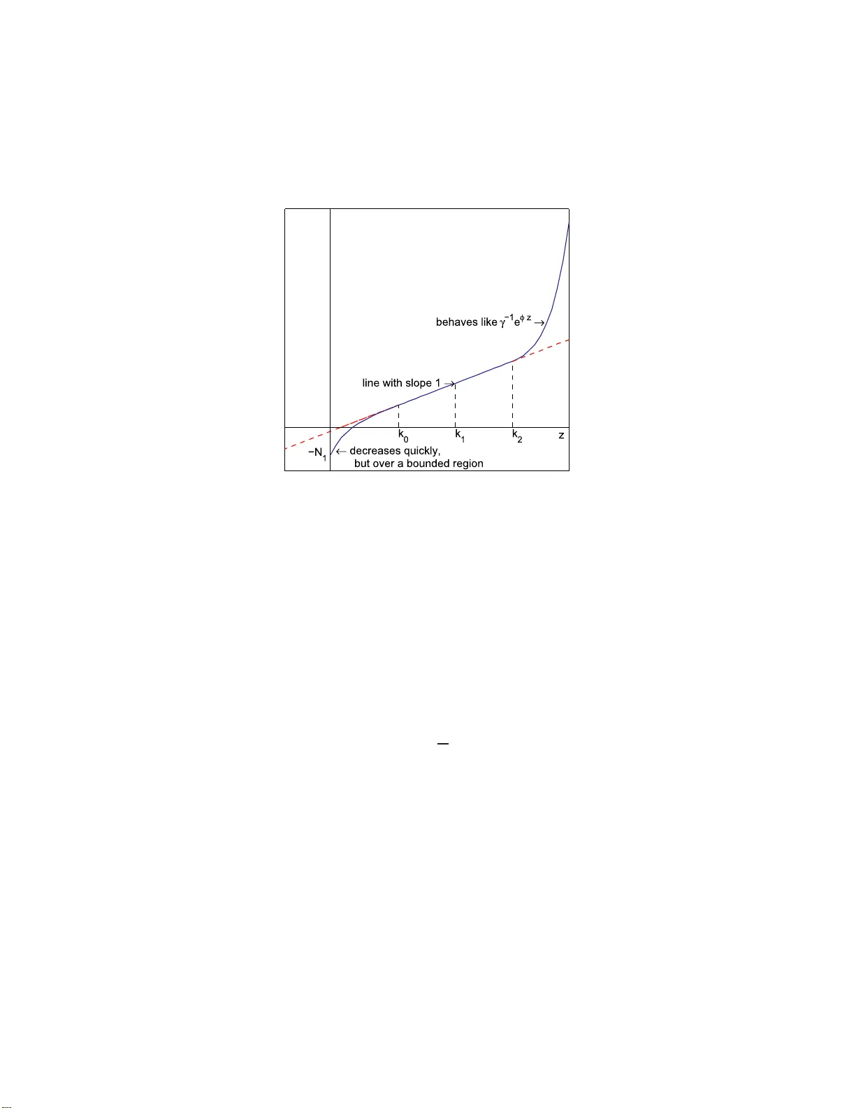
The Annals of Applie d Pr obabil ity 2013, V ol. 23, N o. 5, 1841 –1878 DOI: 10.1214 /12-AAP888 c  Institute of Mathematical Statistics , 2 013 DECA Y OF T AILS A T EQUILIBRIUM F OR FIF O JOIN THE SHOR TEST QUEUE NETWO RKS By Maur y Bramso n 1 , Yi Lu and Balaji Prabhakar 2 University o f Minnesota, University of Il linois and Stanfor d Univ ersity In join the shortest queue netw orks, incoming jobs are assig ned to the shortest queue from among a rand omly chosen subset of D queues, in a system of N queues; after completion of service at its queue, a job leav es the netw ork. W e also assume th at jobs arrive into the system according to a rate- αN P oisson process, α < 1, with rate-1 service a t eac h queue. When the service at queues is exp onential ly dis- tributed, it wa s sho wn in Vvedensk ay a et al. [ Pr obl. Inf. T r ansm. 32 (1996) 15–29] th at the tail of the equ ilibrium queue size decays doubly exp onentiall y in the limit as N → ∞ . This is a substantial improve- ment ov er the case D = 1, where t h e queue size decays exp onential ly . The reasoning in [ Pr obl. I nf. T r ansm. 32 (1996) 15–29] do es not easily generalize to jobs with nonexp onential service time distribu- tions. A mod ularized program for treating general service time distri- butions was introdu ced in Bramson et al. [In Pr o c. ACM SIGMET- RICS (2010) 275–286]. The program relies on an ansatz that asserts, in equilibrium, any ﬁxed number of q ueues b ecome indep endent of one another as N → ∞ . This ansatz wa s demonstrated in several set- tings in Bramson et al. [ Queueing Syst. 71 (2012) 247–292] , including for netw orks where the service discipline is FIFO and the service time distribution h as a decreasing hazard rate. In th is article, we inv estigate the limiting b ehavior, as N → ∞ , of the equilibrium at a queue when the service discipline is FIFO and the service time distribution h as a p ow er law with a giv en exp onent − β , for β > 1. W e show under the ab ov e ansatz that, as N → ∞ , th e tail of t h e equ ilibrium queue size ex hibits a wide range of b ehavior dep ending on th e relationship b etw een β and D . I n particular, if β > D/ ( D − 1), the tail is doubly exp onentia l and, if β < D / ( D − 1), the tail h as a p o w er la w. When β = D / ( D − 1), the t ail is exp on entially distributed. Received June 2011; rev ised Ap ril 2012. 1 Supp orted in part by NSF Gran ts CCF-0729537 and D MS-11-05668. 2 Supp orted in part by NSF Grant CCF-0729537 and by a grant from th e Clean Slate Program at Stanford Universit y . AMS 2000 subje ct classiﬁc ations. 60K25, 68M20, 90B15. Key wor ds and phr ases. Join the shortest qu eu e, FIFO, decay of t ails. This is an electro nic reprint o f the or iginal article published by the Institute of Mathematical Statistics in The Annals of Applie d Pr ob ability , 2013, V ol. 23, No. 5, 1841– 1878 . This r e print diﬀers from the origina l in pagination and typog raphic detail. 1 2 M. BRAMSON , Y. LU AND B. PRA BHAKAR 1. In tro d uction. W e consider join the shortest queue (JSQ) net works, where incoming “jobs” (or “customers”) are assigned to the shortest queue from among D distinct qu eues, D ≥ 2 , with these qu eues b eing chosen u ni- formly from among the N queues in the system, with D ≤ N . When t w o or more of these queues eac h h av e the fewe st num b er of jobs, eac h of the queues is c h osen with equal probability . After completion of service at its queue, a job lea ve s the net w ork. W e assume that j ob s arrive according to a rate- αN P oisson pro cess, α < 1 , and that jobs are served indep en den tly and at r ate 1 at eac h queue. W e are intereste d in th is article in th e case where the service discipline at eac h queue is ﬁr st-in, ﬁr st-out (FIF O ). When the service at queues is exp onen tially distributed, the ev olution of the system is giv en by a counta b le state Marko v c h ain w h ere a state is giv en b y the num b er of j obs at eac h queue. It is not diﬃcult to show that a un ique equilibrium distribution exists; this equilibrium is exc han geable with resp ect to the orderin g of th e queues. Let P ( N ) k denote the probability that th ere are at least k jobs in equilibr ium for the system with N queues. It w as shown in Vvedensk ay a et al. [ 16 ] that lim N →∞ P ( N ) k = α ( D k − 1) / ( D − 1) for k ∈ Z + ; (1.1) in particular, the r igh t tail of P ( N ) k deca ys d oubly exp onentia lly fast in the limit as N → ∞ . T his b eha vior is a substantia l imp r o vemen t o v er the case D = 1, where P ( N ) k deca ys exp onen tially , and h as led to substantia l in ter- est in JS Q netw orks in the literature. F or other references, see Azar et al. [ 1 ], Graham [ 8 ], Luczak–McDiarmid [ 9 , 10 ], Martin–Suh o v [ 11 ], Mitzenma- c her [ 12 ], Su ho v–Vvedensk ay a [ 14 ], V o c king [ 15 ] and Vv edensk ay a–Suho v [ 17 ]. Little w ork has b een d on e on the b eha vior of JS Q net works wh en the ser- vice times are not exp onentia lly distributed. In th is setting, the und erlying Mark o v pr o cess will t yp ically hav e an un coun table state space, and p ositiv e Harris recurrence for the pro cess is no longer obvio us. The latter was sho wn in F oss–Chern o v a [ 7 ], and un iform b ounds on the equilibria w ere shown in Bramson [ 3 ]. (Both articles also considered JSQ n et works with more general arriv als and routing of jobs .) This pap er builds on previous work [ 3 , 4 ] and [ 5 ] by the authors . Bram- son et al. [ 4 ] describ ed a m o dularized program for analyzing the limiting b ehavio r of the equilibria of a family of JSQ netw orks w ith general service times, as N → ∞ . An imp ortant step is to sh o w that any ﬁxed n um b er of queues b ecome indep end en t of one another, with eac h conv erging to a lim- iting distribution that is the equilibrium for an asso ciated Marko v pro cess with a single queue, whic h is a c avity pr o c ess . This pr o cess corresp ond s, in an appropr iate sense, to “setting N = ∞ ” in th e JSQ n et work and viewing the corresp onding inﬁnite dimensional pro cess at a single queue. W e w ill JOIN THE SHOR TEST QU EUE 3 refer to this equilibriu m as the e quilibrium envir onment . In Section 2 , we will p recisely d eﬁne th is terminology . Although it seems that th is indep end ence shou ld hold in a v ery general setting, in clud ing un d er a wid e range of service d isciplines, d emonstrating it app ears to b e a d iﬃ cu lt pr oblem. In Bramson et al. [ 4 ], this ind ep endence and con vergence to the equ ilibrium environmen t w ere stated as an ansatz. This ansatz w as demonstrated in Bramson et al. [ 5 ] in sev eral settings in- cluding for n et works where the service discipline is FIF O and the service distribution has a decreasing hazard rate. In this article, w e emplo y the r estriction of the ab o ve ansatz to FIFO net works. This version of the ansatz will b e precisely stated in Section 2 . Here, we summ arize it for application in the current section: F or a family of net works with the FIF O service d iscipline that are all in equilibrium, an y ﬁxed n u mb er of queues b ecome in- dep end en t in th e limit as N → ∞ . Moreo ve r, eac h marginal distribution con verges to the unique asso ciated equilibriu m en- vironmen t. (1.2) Although th is ansatz has only b een demonstrated for service d istributions ha ving decreasing hazard rate and for general service distributions when the arr iv al rate α is suﬃcien tly small, our argu m en ts here do not other- wise require either restriction. Other applications of the ansatz, bu t for the pro cessor sharing and LIF O service disciplin es, are giv en in [ 4 ]. Our goal, in this article, is to inv estigat e the limiting b ehavio r of the right tail of the asso ciated equilibr ium environmen t, un der the FIF O service disci- pline and with the assigned m ean- 1 service distrib ution F ( · ). Denote b y P k the probabilit y that there are at least k job s in the equilibrium en vironm en t. W e will show that, when F ( · ) h as a p o w er la w tail with exp onent − β , for giv en β > 1, the tail of P k exhibits a wide range of b eha vior dep ending on the relationship b etw een β and D . In particular, if β > D / ( D − 1), the tail is doub ly exp onential and , if β < D / ( D − 1), the tail has a p ow er la w; w h en β = D / ( D − 1), the tail is exp onenti ally distributed. When β ր ∞ , the co- eﬃcien t q D ( β ) of k in the doub ly exp onen tial tail con verge s to 1 , which is the co eﬃcien t of k in ( 1.1 ). On e obtains the same co eﬃcien t of k whether F ( · ) has an exp onen tial tail or has b oun ded supp ort. O ur main resu lts are Theorems 1.1 , 1.2 an d 1.3 . Th eorem 1.1 co vers the case β > D / ( D − 1), The- orem 1.2 co v ers the case β < D / ( D − 1) and Theorem 1.3 co vers the case β = D / ( D − 1). W e set ¯ F ( s ) = 1 − F ( s ). Theorem 1.1. Consider a family of JSQ networks, with giv en D ≥ 2 and N = D , D + 1 , . . . , wher e the N th network has Poisson r ate- αN input, with α < 1 , and wher e servic e at e ach queue is FIF O, with distribution F ( · ) having me an 1 . Assume that ( 1.2 ) holds and that lim s →∞ log ¯ F ( s ) / log s = − β , (1.3) 4 M. BRAMSON , Y. LU AND B. PRA BHAKAR with β ∈ ( D / ( D − 1) , ∞ ) . Then, lim k →∞ (1 /k ) log D log (1 /P k ) = q D ( β ) (1.4) for some q D ( β ) ∈ (0 , 1) . Mor e over, q D ( β ) is c ontinuous in β and q D ( β ) ր 1 exp onential ly fast as β ր ∞ . (1.5) When ( 1.3 ) holds with β = ∞ , then ( 1.4 ) hold s with q D ( ∞ ) = 1 . Theorem 1.1 implies that, when ¯ F ( s ) ∼ cs − β as s → ∞ , for β ∈ ( D / ( D − 1) , ∞ ) and c > 0 , then P k = exp {− D (1+ o (1)) q D ( β ) k } . Theorem 1.2. Consider a family of JSQ networks as in The or em 1.1 , with ( 1.3 ) inste ad holding for β ∈ (1 , D / ( D − 1)) . Then lim k →∞ log (1 /P k ) / log k = ( β − 1) / [1 − ( D − 1)( β − 1)] . (1.6) Theorem 1.2 implies that, wh en ¯ F ( s ) ∼ cs − β as s → ∞ , for β ∈ (1 , D / ( D − 1)) and c > 0, then P k = k − (1+ o (1)) γ D ( β ) , where γ D ( β ) is the r igh t-hand side of ( 1.6 ). Note that γ D ( β ) ց 0 as β ց 1 and γ D ( β ) ր ∞ as β ր D / ( D − 1). Theorem 1.3. Consider a family of JSQ networks as in The or em 1.1 , with ( 1.3 ) r eplac e d by c 1 ≤ lim s →∞ s D / ( D − 1) ¯ F ( s ) ≤ lim s →∞ s D / ( D − 1) ¯ F ( s ) ≤ c 2 (1.7) for some 0 < c 1 ≤ c 2 < ∞ . Then, for appr opriat e r D ( c 2 ) > 0 and s D ( c 1 ) < ∞ , r D ( c 2 ) ≤ lim k →∞ (1 /k ) log (1 /P k ) ≤ lim k →∞ (1 /k ) log (1 /P k ) ≤ s D ( c 1 ) , (1.8) wher e r D ( c 2 ) ր ∞ as c 2 ց 0 , (1.9) s D ( c 1 ) ց 0 as c 1 ր ∞ . Theorem 1.3 implies that when ¯ F ( s ) ∼ cs − D / ( D − 1) as s → ∞ , then P k de- creases exp onentia lly fast in th e sense of ( 1.8 ). Because of ( 1.9 ), the exp onent dep end s strongly on the c hoice of c . When ¯ F ( · ) satisﬁes ( 1.3 ) for a giv en β > 1, the asymptotic b eha vior of P k b ehav es according to ( 1.4 ) or ( 1.6 ), dep ending on whether D > β / ( β − 1) or D < β / ( β − 1). In applications where there is a sub stan tial p enalt y for a mo derately large num b er of jobs at a qu eue (resulting, e.g., in memory o ve rﬂo w ), it is therefore imp ortant to c ho ose D > β / ( β − 1) . This distinction do es not o ccur when ¯ F ( · ) has an exp onenti al tail, since any c hoice of D ≥ 2 JOIN THE SHOR TEST QU EUE 5 pro du ces a d oubly exp onen tial tail for P k , as in ( 1.1 ). (See [ 4 ] for more detail.) W e p oint out that the p ro ofs of T heorems 1.1 – 1.3 only dep end on ( 1.2 ) for th e existence of an equilibriu m en viron m en t. Regardless of ho w th e ex- istence of an equilibrium en vironm en t is veriﬁed, ( 1.2 ) w ill b e n eeded in order to relate the tail b eha vior of P k for th e equilibrium environmen t to the tail b ehavio r for the equilibria of the corresp onding family of netw orks as N → ∞ . W e also n ote that, although the phr ase “join the sh ortest queue n et work” is widely u sed in the literature, such systems are not true net works in the sense that, up on the d ep arture of a job from a qu eu e, the job lea ves the system instead of b eing able to r eturn to a diﬀeren t queue. Ho we v er, suc h systems hav e b een extended to the setting of J ac kson n et works (see, e.g., [ 11 ] and [ 14 ]). This article is organized as follo ws. In Section 2 , w e pro vide basic b ac k- ground on the prop erties of the state space and Mark o v p ro cess that und erlie the JSQ n et works. W e then deﬁn e equilibrium environmen ts and formally state the ansatz. In S ections 3 – 5 , w e d emonstrate Theorems 1.1 , 1.2 and 1.3 , resp ectiv ely . Our approac h will b e to demons trate low er b ounds and then upp er b ounds that yield the theorem. In eac h case, the lo wer b ound s will b e considerably easier to sho w . Notation. F or the reader’s con venience, we menti on here some of the notation in the pap er. W e w ill emplo y C 1 , C 2 , . . . to d enote p ositive constan ts whose p recise v alue is not of imp ortance to us. F or z ∈ R , ⌊ z ⌋ and ⌈ z ⌉ will denote, resp ectiv ely , the in teger part of z and the smallest intege r at least as large as z . 2. Mark o v pro cess b ac kground , equilibriu m enviro nmen ts and the ansatz. In this section, w e pro vide a more detailed description of the construction of the Mark o v pro cesses X ( N ) ( · ) that underlie th e JS Q netw orks. W e next deﬁne the corresp onding cavit y pro cess and its equilibr iu m environmen t. W e then emplo y these concepts to state the ansatz for JSQ net wo rks. Most of this material is included in Sections 2 and 3 of Bramson et al. [ 5 ]. (Related material is also giv en in [ 2 ] and [ 3 ].) W e d eﬁne the state space S ( N ) to b e the set ( Z × R 2 ) N . (2.1) The ﬁrst coord inate z n , n = 1 , . . . , N , corresp onds to the num b er of jobs at the n th queue; the second co ordinate u n , u n ≥ 0, is the amoun t of time the oldest job there h as already b een served; and the last co ordinate s n , s n > 0, is the residual service time. When z n = 0, set the other t w o co ordinates equal to 0. Th e co ordin ate u n will not play a role in the evol ution of X ( N ) ( · ) here; 6 M. BRAMSON , Y. LU AND B. PRA BHAKAR w e r etain it for comparison with [ 5 ], wh ere it was used to demonstr ate ( 1.2 ) under decreasing hazard rates. (W e will emp lo y sligh tly diﬀerent notation here than in [ 5 ].) F or giv en N ′ ≤ N , S ( N ′ ) is the pr oje c tion of S ( N ) obtained b y restricting S ( N ) to the ﬁ r st N ′ queues; for x ∈ S ( N ) , x ′ ∈ S ( N ′ ) is thus obtained b y omit- ting the co ordin ates w ith n > N ′ . On e can also deﬁne pro jections of S ( N ) on to spaces S ( N ′ ) corresp ondin g to other sub sets of { 1 , . . . , N } analogously , although th ese are not needed here. W e deﬁne the metric d ( N ) ( · , · ) on S ( N ) , with d ( N ) ( · , · ) giv en in terms of d ( N ) ,n ( · , · ) b y d ( N ) ( · , · ) = (1 / N ) P N n =1 d ( N ) ,n ( · , · ). F or giv en x 1 , x 2 ∈ S ( N ) , with the co ordinates lab elled corresp ond ingly , set d ( N ) ,n ( x 1 , x 2 ) = | z n 1 − z n 2 | + | u n 1 − u n 2 | + | s n 1 − s n 2 | . (2.2) One can c h eck that the metric d ( N ) ( · , · ) is separable and lo cally compact; more detail is giv en on page 82 of [ 2 ]. W e equip S ( N ) with the standard Borel σ -algebra inh erited from d ( N ) ( · , · ), which w e denote b y S ( N ) . The Mark o v pro cess X ( N ) ( t ), t ≥ 0, underlyin g a giv en mo d el is deﬁn ed to b e the righ t contin uous p r o cess with left limits, taking v alues x in S ( N ) , whose ev olution is determined by the mo del together with th e assigned ser- vice discipline. W e denote the rand om v alues of th e co ord inates z n , u n and s n tak en b y X ( N ) ( t ), by Z n ( t ), U n ( t ) and S n ( t ). Jobs are allo cated service according to the FIFO discipline; durin g the p erio d a j ob is b eing served, U n ( t ) increases at rate 1 and S n ( t ) decreases at rate 1. Along the lines of page 85 of [ 2 ], a ﬁltration ( F ( N ) t ), t ∈ [0 , ∞ ], can b e assigned to X ( N ) ( · ) so that X ( N ) ( · ) is a piecewise-deterministic Mark o v pro cess, and hence is Borel righ t. This implies that X ( N ) ( · ) is strong Mark o v. (W e d o n ot otherwise use Borel right .) The r eader is referred to Davis [ 6 ] for more detail. Equilibrium env i r onments and the ansatz. In ord er to state th e ansatz, w e requ ire s ome termin ology . W e denote b y E ( N ,N ′ ) the p ro jection of the equilibrium m easure E ( N ) of the N -queue system on to the ﬁrst N ′ queues. [Since X ( N ) ( t ) is exc hangeable when X ( N ) (0) is, the c hoice of queues will not m atter.] W e wish to describ e th e ev olution of individual qu eu es for the limiting pro cess, as N → ∞ . F or this, we construct a strong Mark o v p r o cess X H ( t ), t ≥ 0 , on S (1) . W e will deﬁne X H ( t ) sim ilarly to X (1) ( t ), except that only a fraction of in coming p oten tial arriv als at the qu eue is p ermitted to arrive at the queue, with the f raction dep ending on the current num b er of jobs there, and w ith the fraction decreasing as the n umb er of jobs increases. W e pro ceed as follo ws . Let H denote a prob ab ility measure on S (1) , whic h w e refer to as the envir onment of the pro cess X H ( · ); we refer to X H ( · ) as the JOIN THE SHOR TEST QU EUE 7 asso ciated c avity pr o c ess . W e deﬁne X H ( · ) so that p otential arrivals arrive according to a rate- D α P oisson p ro cess. When suc h a p oten tial arr iv al to the qu eue o ccurs at time t , X H ( t − ) is compared w ith the states of D − 1 indep en d en t random v ariables, eac h with la w H ; we r efer to these D − 1 states at a p oten tial arriv al as the c omp arison states . Ch o osing from among these D states, the job is assigned to the state with the few est num b er of jobs. (In case of a tie, eac h of these states is c h osen w ith equal p robabilit y .) If the job has chosen the state X H ( t − ) at the queue, it then immediately joins the queue; otherwise, the job imm ed iately lea ves the system. In either case, the indep endent D − 1 states employ ed for this purp ose are imm ediately discarded. W e giv e the follo wing illustrations, d enoting by Q k the probability that the en vironmen t H h as at least k jobs . F or D = 2 , if a p otentia l arriv al o ccurs at time t and X H ( t − ) = k , then the p robabilit y that X H ( t ) = k + 1 is ( Q k + Q k +1 ) / 2, and so the rate α k of an arriv al at the queue is α ( Q k + Q k +1 ). F or general D , in ord er for a p oten tial arriv al to arriv e at the queue, it is necessary for all of the D − 1 comparison states used at that time to b e at least k , in wh ic h case the probabilit y of selecting the queue is the r ecipr o cal of th e num b er of states equ al to k . This give s the b ounds αQ D − 1 k ≤ α k ≤ αD Q D − 1 k . (2.3) W e assume that jobs in the ca vit y pr o cess X H ( · ) hav e the same service distribution F ( · ) as in the qu eueing net work and are serv ed according to the FIF O service discipline. Th e n u m b er of jobs in X H ( t ) will b e denoted by Z H ( t ), the amoun t of time the oldest job has already b een served b y U H ( · ) and th e r esidual serv ice time by S H ( t ); we will employ x , z , u and s for the corresp ondin g terms in the state sp ace. When a ca vit y pro cess X H ( · ), with environmen t H , is stationary with the equilibrium measure H [i.e., X H ( t ) has the distribution H for all t ], w e sa y th at H is an e quilibrium envir onment . One can think of an equilibr ium en viron m en t as b eing the restriction of an equilibrium measure for the JSQ net work, viewe d at a s ingle qu eue, when “the total n u mb er of qu eues N is inﬁnite.” More bac kground on the ca vit y p r o cess is giv en in [ 4 ]. W e n o w state the ansatz. Here, v → on S ( N ′ ) denotes conv ergence in total v ariation w ith resp ect to th e m etric d N ′ ( · , · ) on S ( N ′ ) . Ansa tz. Consider a family of JSQ networks, with given D ≥ 2 and N = D , D + 1 , . . . , wher e the N th network has Poisson r ate- αN input, with α < 1 , and wher e servic e at e ach queue is FIF O, with distribution F ( · ) hav- ing me an 1 . Then, (a) for e ach N ′ , E ( N ,N ′ ) v → E ( ∞ ,N ′ ) as N → ∞ , (2.4) wher e E ( ∞ ,N ′ ) is the N ′ -fold pr o duct of E ( ∞ , 1) . Mor e over, (b) E ( ∞ , 1) is the unique e quilibriu m envir onment asso ciate d with this family of networks. 8 M. BRAMSON , Y. LU AND B. PRA BHAKAR As w as m en tioned in the In tro duction , this ansatz wa s demonstrated in Bramson et al. [ 5 ] when the service time distribu tion F ( · ) has a decreasing hazard rate h ( · ) [i.e., h ( s ) = F ′ ( s ) / ¯ F ( s ) is n onincreasing in s ] and for general service distributions wh en the arriv al r ates are small enough. In order to demonstrate Theorems 1.1 – 1.3 , we w ill analyze the cavit y pro cess X H ( · ) with its u nique equ ilibrium environmen t H = E ( ∞ , 1) . I n p ar- ticular, w e will analyze E ( ∞ , 1) o ve r a cycle starting and ending at the state 0. (The state where the n u m b er of jobs z is 0.) Letting ν denote the time at wh ic h X H ( · ) ﬁr st retur ns to 0 after visiting another state, the ﬁ r st cycle is the random time in terv al [0 , ν ]. F or an y k ≥ 1 , w e will d enote b y V k the o c c u p ation time at states x , with z ≥ k , o v er [0 , ν ], that is, V k = Z ν 0 1 { Z H ( t ) ≥ k } dt. Setting m 0 = E [ ν ], the mean return time to 0, one has P k = m − 1 0 E [ V k ] , (2.5) where P k is the p robabilit y there are at least k jobs in the equilibrium en viron m en t. Letting α k denote th e arriv al rate of jobs for X H ( · ) when z = k , one h as αP D − 1 k ≤ α k ≤ αD P D − 1 k , (2.6) whic h is th e analog of ( 2.3 ). Sin ce the departur e of jobs from the queue is deterministic, b eing a f unction of the residual service time s , ( 2.6 ) giv es a rea- sonably explicit d escription of the tr an s ition rates for X H ( · ). T ogether w ith ( 2.5 ), ( 2.6 ) w ill provide the basis for our d emonstration of Theorems 1.1 – 1.3 and w ill b e u sed throughout the pap er. 3. The case where β > D / ( D − 1) . In this section, we demonstrate Theorem 1.1 ; w e do this by demonstrating lo w er and u pp er b ound s that are needed for the theorem in Prop ositions 3.1 and 3.2 . Eac h of these b ounds is expressed in terms of a recurs ion relation f or P k . In order to obtain T he- orem 1.1 from these r ecursions, w e emplo y Prop osition 3.3 , w hic h analyzes suc h r ecursions by u tilizing a standard f ramew ork inv olving rational gener- ating fun ctions. T he section is organized as follo ws. After stating Prop osi- tions 3.1 and 3.2 , w e state and p ro ve Prop osition 3.3 . W e next emp lo y the three prop ositions to demonstrate Theorem 1.1 . W e then provide the rela- tiv ely q u ic k pro of of Pr op osition 3.1 and the longer pro of of Pr op osition 3.2 , in the follo win g subsections. In b oth prop ositions, w e set k 1 = ⌈ k − β ⌉ (or, equ iv alen tly , ⌊ β ⌋ = k − k 1 ) and ˆ β = β − ⌊ β ⌋ . Pr oposition 3.1. Consider a family of JSQ networks, with given D ≥ 2 and N = D , D + 1 , . . . , wher e the N th network has Poisson r ate- αN input, with α < 1 , and wher e servic e at e ach queue is FIF O, with distribution F ( · ) JOIN THE SHOR TEST QU EUE 9 having me an 1 . Assume that ( 1.2 ) holds. Then, for appr opriate C 1 > 0 and al l k , P k ≥ ( C 1 / 8 k ) k k − 1 Y i =0 P D − 1 i . (3.1) If mor e over, for some s 0 ≥ 1 , ¯ F ( s ) ≥ s − β for s ≥ s 0 , (3.2) with β ∈ ( D / ( D − 1) , ∞ ) , then, for appr opriate C 1 > 0 and al l k , P k ≥ C 1 3 − k k − 1 Y i = k 1 +1 P D − 1 i ! P ˆ β ( D − 1) k 1 . (3.3) Pr oposition 3.2. Consider a family of JSQ networks, with given D ≥ 2 and N = D , D + 1 , . . . , wher e the N th network has Poisson r ate- αN input, with α < 1 , and wher e servic e at e ach queue is FIF O, with distribution F ( · ) having me an 1 . Assume that ( 1.2 ) holds and that, for some s 0 ≥ 1 , ¯ F ( s ) ≤ s − β for s ≥ s 0 , (3.4) with β ∈ ( D / ( D − 1) , ∞ ) . If β is not an inte ger, then, for appr opriate C 2 and al l k , P k ≤ C 2 k β +1 k − 1 Y i = k 1 +1 P D − 1 i ! P ˆ β ( D − 1) k 1 . (3.5) If β is an inte ger, then, for e ach δ > 0 , appr opriate C 2 and al l k , P k ≤ C 2 k β +1 k − 1 Y i = k 1 +2 P D − 1 i ! P (1 − δ )( D − 1) k 1 +1 . (3.6) T o emplo y the recursions in ( 3.3 ) and ( 3.5 )–( 3.6 ) of Pr op ositions 3.1 and 3.2 in the pro of of Theorem 1.1 , w e will analyze the asymptotic b e- ha vior of the recur sions in ( 3.7 ). Pr oposition 3.3. Supp ose that R k satisﬁes R k = ( D − 1) k − 1 X i = k − ℓ +1 R i + η R k − ℓ ! for k ≥ 1 , (3.7) with R k = 1 for k = − ℓ + 1 , . . . , − 1 , 0 , wher e ℓ, D ≥ 2 and η ∈ [0 , 1] . Then, setting β = ℓ + η − 1 , lim k →∞ 1 k log D R k = q D ( β ) (3.8) for some q D ( β ) ∈ (0 , 1) . M or e over, q D ( β ) is c ontinuous in β and q D ( β ) ր 1 exp onential ly fast as β ր ∞ . 10 M. BRAMSON , Y. LU AND B. PRA BHAKAR Pr oof. The recur rence ( 3.7 ) is a sp ecial case of linear r ecursions of the form R k + ℓ X i =1 a i R k − i = 0 , (3.9) with a i ∈ C an d general R − ℓ +1 , . . . , R 0 . It is w ell known that (see, e.g., Stan- ley [ 13 ], p age 202) R k = j X i =1 P i ( k ) γ k i (3.10) for eac h k , wh ere γ i are distinct, P i ( k ) is a p olynomial in k of degree strictly less th an ℓ i , and 1 + ℓ X i =1 a i x i = j Y i =1 (1 − γ i x ) ℓ i , (3.11) with P j i =1 ℓ i = ℓ . Moreo ve r the con verse holds, that is, if ( 3.10 ) and ( 3.11 ) b oth hold, then so do es ( 3.9 ). F or R k giv en b y ( 3.7 ), it is n ot diﬃcult to chec k that there is exactly one v alue γ i , sa y γ 1 , that is real and p ositiv e, that γ 1 v aries contin uously in η , and moreo ver that γ 1 satisﬁes γ 1 > 1, since a i < 0 and P ℓ i =1 a i < − 1. (Descartes’ rule of signs in fact implies that 1 /γ 1 is a simple r o ot.) Also, b ecause a i < 0, and p ossesses b oth o d d an d ev en indices, | γ i | < γ 1 for i 6 = 1. Since the initial data give n b elow ( 3.7 ) are all p ositiv e, any solution of ( 3.7 ) is ma jorized b y this particular solution, up to a m ultiplicativ e constan t; so, P 1 ( · ) 6≡ 0. The limit in ( 3.8 ), with q D ( β ) = log D γ 1 > 0, follo ws from these observ ations. W e still need to examine the limiting b eha v ior of q D ( β ) as β → ∞ . Divid- ing b oth sides in ( 3.7 ) by R k , then sub stituting ( 3.10 ) for eac h of the term s , and letting k → ∞ implies that 1 = ( D − 1)( x + x 2 + · · · + x ℓ − 1 + η x ℓ ) = ( D − 1)( x − (1 − η ) x ℓ − η x ℓ +1 ) / (1 − x ) for x = 1 /γ 1 = D − q D ( β ) . T his again uses γ 1 > | γ i | for i 6 = 1 . Hence, D x − 1 = ( D − 1)((1 − η ) x ℓ + η x ℓ +1 ) . (3.12 ) Note that x ∈ (0 , 1) and that, since q D ( β ) is increasing in β , x is d ecreasing in β . Since the r igh t-hand side go es to 0 exp onent ially fast as ℓ ր ∞ , and hence as β ր ∞ , it follo ws that x ց 1 /D exp onentially fast as β ր ∞ , which also implies q D ( β ) ր 1 exp onen tially fast, as desired. Note that the precise exp onentia l r ate of con vergence can b e obtained by inserting this limit bac k in to the righ t-hand side of ( 3.12 ).  JOIN THE SHOR TEST QU EUE 11 Applying Prop osition 3.3 to Prop ositions 3.1 and 3.2 , we n o w demonstrate Theorem 1.1 . Pr oof of The orem 1.1 . Setting Q k = e R k , wh ere R k is give n in ( 3.7 ), one h as Q k = k − 1 Y i = k − ℓ +1 Q D − 1 i ! Q η ( D − 1) k − ℓ , (3.13) with Q k = e for k = − ℓ + 1 , . . . , − 1 , 0. W e pro ceed to compare Q k with 1 /P k , where P k satisﬁes on e of ( 3.3 ), ( 3.5 ) and ( 3.6 ). Comparison of Q k with 1 /P k , with η = ˆ β , ℓ = ⌊ β ⌋ = k − k 1 and P k satisfy- ing ( 3.3 ), provides an upp er b ound on th e limit in ( 1.4 ). T o see th is, w e ﬁ rst set ˜ Q k = M − k Q k , for giv en M > 1 . Sin ce ( D − 1)( β − 1) > 1, by sub stituting in to ( 3.13 ), one can c hec k th at, for large enough M and k , ˜ Q k ≥ C 3 b k k − 1 Y i = k − ℓ +1 ˜ Q D − 1 i ! ˜ Q η ( D − 1) k − ℓ (3.14) for an y ﬁxed c hoice of C 3 and b , in particular, for C 3 = 1 /C 1 and b = 3, where C 1 is c hosen as in Prop osition 3.1 . Moreo v er, on account of ( 3.8 ), lim k →∞ (1 /k ) log D log ( ˜ Q k ) = q D ( β ) , (3.15) where, in p articular, q D ( β ) > 0 , and hence ˜ Q k → ∞ as k → ∞ . W e observe that 1 /P k satisﬁes the inequ alit y that is analogous to that for P k in ( 3.3 ), bu t with the inequality rev ersed and prefactors 3 k /C 1 instead of C 1 / 3 k . Comparing ˜ Q k with 1 /P k therefore implies that, for large enou gh n not d ep end ing on k , 1 /P k ≤ ˜ Q k + n . The upp er b ound for ( 1.4 ) th erefore follo ws from ( 3.15 ) for th e s ame choice of q D ( β ), whic h we recall is con tinuous in β . T he limit in ( 1.5 ) also follo ws from Pr op osition 3.3 . Comparison of Q k with 1 /P k also pr o vides a lo wer b ound on the limit in ( 1.4 ). In the case where β is noninteg ral, w e c ho ose η and ℓ as b efore, with η = ˆ β , ℓ = ⌊ β ⌋ = k − k 1 ; note that P k satisﬁes the up p er b ound in ( 3.5 ). W e pro ceed as in the ﬁrst part, bu t instead set ˜ Q k = M k Q k , for giv en M > 1 . One can c hec k that, for large enough M and k , ˜ Q k ≤ C 3 b k k − 1 Y i = k − ℓ +1 Q D − 1 i ! Q η ( D − 1) k − ℓ (3.16) for any c h oice of C 3 > 0 and b > 0. As b efore, ( 3.15 ) holds. The terms 1 /P k satisfy the inequalit y that is the analog of ( 3.5 ). Also, 1 /P k → ∞ as k → ∞ . Comp arin g ˜ Q k with 1 /P k therefore implies that, for 12 M. BRAMSON , Y. LU AND B. PRA BHAKAR large enough n not dep en ding on k , 1 /P k + n ≥ ˜ Q k . (3.17) The lo wer b ound for ( 1.4 ) therefore follo ws from ( 3.15 ) when β is nonin tegral. The reasoning in th e case where β is inte gral is similar, but with the diﬀerence that we n o w choose η = 1 − δ , ℓ = β − 1 = k − k 1 − 1 , where δ ∈ (0 , 1) is arb itrary . No w , P k satisﬁes the upp er b ound in ( 3.6 ). W e pro ceed as in the nonint egral case, once again obtaining ( 3.16 ). Comparing 1 /P k with ˜ Q k again pro du ces ( 3.15 ), except that th e limit is no w q D ( β − δ ) b ecause of our choic e of η . By Pr op osition 3.3 , q D ( · ) is con tin uous in its argument. Therefore, letting δ ց 0 p ro du ces the s ame limit as in the noninteg ral case, and h ence implies the low er b ound for ( 1.4 ) in the case where β is in tegral. W e still need to demonstr ate that when ( 1.3 ) h olds with β = ∞ , then ( 1.4 ) holds with q D ( ∞ ) = 1 . The low er b ound in ( 1.4 ) h olds on account of ( 1.5 ). T he up p er b ound is n ot diﬃcult to sh o w and do es n ot require Prop osition 3.3 ; we pro ceed to show the b ound. W e will sho w by induction that, for all k , P k ≥ ( C 1 / 8 k ) k D k , (3.18) where C 1 is as c h osen as in ( 3.1 ), wh ic h we assume WLOG is at most 1 . T o see ( 3.18 ), note that if it holds for all i = 0 , . . . , k − 1 then this, together with ( 3.1 ), implies that P k ≥ ( C 1 / 8 k ) k k − 1 Y i =0 [( C 1 / 8 i ) iD i ] D − 1 ≥ ( C 1 / 8 k ) ( k − 1)( D k − 1)+ k ≥ ( C 1 / 8 k ) k D k . The upp er b oun d in ( 1.4 ), with q D ( ∞ ) = 1, follo ws immed iately from ( 3.18 ).  Demonstr ation of Pr op osition 3.1 . The pro of of Pr op osition 3.1 is qu ic k. T o obtain the lo wer b ounds in b oth ( 3.1 ) and ( 3.3 ), it su ﬃ ces to construct a path along whic h Z H ( t ) increases from 0 to k within th e ﬁrst cycle. This is done, in b oth cases, by allo cating the same amount of time to eac h of the ﬁrst k arriv als, wh ic h are also required to o ccur b efore the ﬁr s t departure. Pr oof of Proposition 3.1 . Consider th e ca v ity pro cess X H ( · ) with X H (0) = 0 . In order to show ( 3.1 ) and ( 3.3 ), w e obtain lo wer b ounds on the exp ected amount of time E [ V k ] o ver w h ic h Z H ( t ) ≥ k b efore X H ( · ) returns to 0. W e ﬁr st sho w ( 3.1 ). W e consider the eve n t A where the ﬁ rst service time S is at least 1 / 2 and the ﬁ rst k arriv als o ccur b y time 1 / 4. The latter even t con tains the eve n t JOIN THE SHOR TEST QU EUE 13 where eac h of the ﬁr st k arriv als o ccurs not more than 1 / 4 k un its of time after th e pr evious arriv al, starting at time 0. Conditioned on th ere b eing i jobs in the queue, jobs arr iv e at rate α i ≥ αP D − 1 i , and so the probabilit y of suc h an arr iv al o ccurr in g o ve r an in terv al of length 1 / 4 k is at least 1 − exp {− αP D − 1 i / 4 k } . So, give n th at S ≥ 1 / 2, the probabilit y that all k of these arriv als o ccur by time 1 / 4 is at least k − 1 Y i =0 (1 − exp {− αP D − 1 i / 4 k } ) . (3.19) The even t S ≥ 1 / 2 o ccurs with some p ositiv e pr ob ab ility c d ep endin g on F ( · ) and, under the even t A , the departur e time for the ﬁ rst job o ccurs at least 1 / 4 after the last of the ﬁ rst k arriv als. So, the exp ected amoun t of time in [1 / 4 , 1 / 2], d uring which Z H ( t ) ≥ k and b efore X H ( · ) h as return ed to 0, is at least c 4 k − 1 Y i =0 (1 − exp { − αP D − 1 i / 4 k } ) , (3.20) whic h is therefore a low er b oun d for E [ V k ]. It therefore follo w s from ( 2.5 ) that P k ≥ c 4 m 0 k − 1 Y i =0 (1 − exp {− αP D − 1 i / 4 k } ) ≥ c 4 ( α/ 8 k ) k k − 1 Y i =0 P D − 1 i , (3.21) whic h implies ( 3.1 ) f or appropr iate C 1 . W e n ext show ( 3.3 ) un der the assumption ( 3.2 ). F or this, w e set s 1 = 2 k / ( αP D − 1 k 1 ) . (3.22) One can reason analogously as th r ough ( 3.20 ), but by replacing the time in terv al [0 , 1 / 2] b y [0 , s 1 ] and emplo ying s 1 / 2 k for the allotted time for eac h of the k arriv als. One obtains that the exp ected amount of time in [ s 1 / 2 , s 1 ], during wh ic h Z H ( t ) ≥ k and b efore X H ( · ) has retur n ed to 0, is at least s 1 2 ¯ F ( s 1 ) k − 1 Y i =0 (1 − exp {− αs 1 P D − 1 i / 2 k } ) . (3.23) Cho ose k large enough so that s 1 ≥ s 0 , where s 0 is as in ( 3.2 ) and s 1 is as in ( 3.22 ). Since e − x ≤ (1 − x/ 2) ∨ 1 / 2 f or x ≥ 0, this is at least 2 − ( k 1 +2) s − ( β − 1) 1 ( αs 1 / 4 k ) k − k 1 − 1 k − 1 Y i = k 1 +1 P D − 1 i ≥ 2 − k ( α/ 4 k ) β k − 1 Y i = k 1 +1 P D − 1 i ! P ˆ β ( D − 1) k 1 , 14 M. BRAMSON , Y. LU AND B. PRA BHAKAR where th e inequalit y follo ws from ( 3.22 ) and k − k 1 = β − ˆ β . Consequently , E [ V k ] ≥ 2 − k ( α/ 4 k ) β k − 1 Y i = k 1 +1 P D − 1 i ! P ˆ β ( D − 1) k 1 . Again applying ( 2.5 ), it follo ws that, for large enough k (dep ending on α and β ), P k ≥ 3 − k k − 1 Y i = k 1 +1 P D − 1 i ! P ˆ β ( D − 1) k 1 , whic h implies ( 3.3 ).  Demonstr ation of Pr op osition 3.2 . In ord er to demons trate Prop osi- tion 3.2 , we will emp lo y Lemma 3.1 b elo w; th e lemma w ill also b e emp lo ye d in the demonstration of Prop ositions 4.2 and 5.2 . (A substantia lly more in- tricate v arian t of the pro of of Lemma 3.1 w ill b e n eeded for the p r o of of Prop osition 4.4 .) L emma 3.1 provides up p er b ounds inv olving R ( k , s ), H ( n ) and ρ ( k , s ), for k ≥ 1, s ≥ 0 and n ≥ 0, wh ic h are deﬁned as follo ws. F or s > 0 , R ( k , s ) is the exp ected retur n time of the cavit y pro cess X H ( · ) (with equilibrium en viron m en t H ) to th e empt y state 0, from X H (0) with Z H (0) = k and S H (0) = s . W e set R ( k , 0) = lim s ց 0 R ( k , s ), whic h is also the exp ected return time to 0 ju st after departur e of a job, but w ith ou t kno wledge of the residual service time of the job that is b eginning service. The quantit y H ( n ) is th e num b er of jobs, for this p ro cess, at the time wh en the ( n + 1)s t job h as just departed, for example, H (0) is the num b er of j ob s just after d eparture of th e job originally in service. The stopping time ρ ( k , s ) is the ﬁrst time n at wh ic h H ( n ) = 0. W e also denote b y Y n the serv ice time of the ( n + 1)st j ob (with Y 0 = s b e- ing the service time of the j ob originally in serv ice), and set T ℓ = P ℓ n =0 Y n = P ℓ n =1 Y n + s . Note th at Y 1 , Y 2 , . . . are i.i.d. with d istribution fun ction F ( · ), whic h , as alw ays, is assumed to ha ve mean 1. Lemma 3.1. L et R ( · , · ) and ρ ( · , · ) b e deﬁne d as ab ove. Then, for lar ge enough N 0 , R ( k , s ) ≤ 2( k + s + N 0 ) (3.24) and E [ ρ ( k , s )] ≤ 2( k + s/ 2 + N 0 ) (3.25) for al l k and s . Pr oof. It is not diﬃcult to see that ( 3.24 ) follo ws from ( 3.25 ). By ap- plying W ald’s equation to T ( · ) and ρ ( · , · ) (with r esp ect to th e und erlying JOIN THE SHOR TEST QU EUE 15 σ -algebra generated b y X H ( · )), one obtains R ( k , s ) = E [ T ρ ( k, s ) ] = E " ρ ( k, s ) X n =1 Y n # + s = E [ ρ ( k , s )] E [ Y 1 ] + s ≤ 2( k + s + N 0 ) , with the inequalit y follo wing fr om ( 3.25 ) and E [ Y 1 ] = 1 . In ord er to sho w ( 3.25 ), w e consider the pro cess M ( n ) = H ( n ) + n / 2 − N 1 exp {− θ ( H ( n ) ∧ k 0 ) } . (3.26) F or appropriate c hoices of N 1 , θ > 0 and k 0 ∈ Z + , w e claim M ( n ) is a su- p ermartingale, w ith r esp ect to the ﬁltration G n = σ ( H (0) , . . . , H ( n )), after restricting to times n , with n ≤ ρ ( k , s ), and then stopping the pr o cess. These three constan ts are c hosen as follo ws. W e c h o ose k 0 large enough so that αD P D − 1 k 0 +1 ≤ 1 / 2. F or H ( n ) > k 0 , one can chec k that the su p ermartin gale inequalit y E [ M ( n + 1) |G n ] ≤ M ( n ) (3.27) is satisﬁed—the arriv al rate of jobs is at most 1 / 2 o ve r the time in terv al ( T n − 1 , T n ] du ring whic h the ( n + 1)st job is served, whic h has mean length 1, and so E [ H ( n + 1) |G n ] ≤ H ( n ) − 1 / 2 . In ord er to analyze M ( n + 1) wh en H ( n ) ≤ k 0 , we set M 1 ( n ) = − exp {− θ ( H ( n ) ∧ k 0 ) } . W e choose θ large enough so that, for some ε > 0 and all H ( n ) ≤ k 0 , E [ M 1 ( n + 1) |G n ] ≤ M 1 ( n ) − ε. (3.28) This requires a standard compu tation u sing the conv exit y of the exp onen tial function and the up p er b ound αD on the arriv al rate of jobs. [S ince H ( · ) ma y hav e p ositiv e drif t, θ ma y need to b e c hosen large.] W e also c ho ose N 1 so that εN 1 ≥ αD + 1 / 2. T ogether with ( 3.28 ), this implies ( 3.27 ) also holds for H ( n ) ≤ k 0 . Consequ en tly , M ( n ) is a sup er- martingale, as claimed. In order to demonstrate ( 3.25 ), w e will app ly the optional sampling the- orem to M ( · ) stopp ed at times ρ n ( k , s ) = ρ ( k , s ) ∧ n . First note that E [ M (0)] ≤ E [ H (0)] ≤ k + s/ 2 (3.29) for k ≥ k 0 , since the arriv al rate of jobs is b ound ed ab o ve b y 1 / 2. Also, for giv en s , E [ H (0)] is increasing as a function of k , the num b er of jobs in the ca vit y pro cess at time 0 . T ogether with ( 3.29 ), this im p lies that, for all k , E [ M (0)] ≤ ( k ∨ k 0 ) + s/ 2 ≤ k + s/ 2 + k 0 . (3.30) Since th e sup ermartingale M ( · ) is b ounded fr om b elo w, app lication of th e optional sampling theorem to ρ n ( k , s ) imp lies that E [ M ( ρ n ( k , s ))] ≤ E [ M (0)] ≤ k + s/ 2 + k 0 , 16 M. BRAMSON , Y. LU AND B. PRA BHAKAR and h ence 0 ≤ E [ H ( ρ n ( k , s ))] ≤ k + s/ 2 + k 0 + N 1 − E [ ρ n ( k , s )] / 2 . Solving for E [ ρ n ( k , s )] imp lies E [ ρ n ( k , s )] ≤ 2( k + s/ 2 + k 0 + N 1 ) = 2( k + s/ 2 + N 0 ) for N 0 = k 0 + N 1 . L etting n → ∞ implies ( 3.25 ).  Lemma 3.1 p ro vides an upp er b ound on th e exp ected time ov er a cycle during whic h there are at least k jobs, p ro vided such a state has already b een attained. Belo w, w e will obtain an upp er b ound on the probabilit y of attaining s uc h a state and com b ine this with ( 3.24 ). In ord er for X H ( · ), s tarting at 0 , to attain a state with k jobs, it must ﬁrs t attain states with k 1 + 1 , k 1 + 2 , . . . , k − 1 jobs , w h ere k 1 has b een sp eciﬁed in the previous su bsection. (It tur ns out that includin g states with few er jobs in th is sequence will n ot impro v e our b ound s.) W e let σ k 1 +1 , . . . , σ k denote the num b er of jobs that ha v e already departed w hen s uc h a s tate is ﬁrst attained [e.g., σ i = 0 m eans that the ﬁ rst job is still b eing served at the time t when Z H ( t ) = i ﬁ rst o ccur s]. One trivially has 0 ≤ σ k 1 +1 ≤ σ k 1 +2 ≤ . . . ≤ σ k . P artition { k 1 + 1 , k 1 + 2 , . . . , k } so that i 6 = i ′ are in the same subs et if σ i = σ i ′ , that is, the times t i and t i ′ at whic h Z H ( t i ) = i and Z H ( t i ′ ) = i ′ ﬁrst o ccur are in the same service time in terv al. One can write such a partition as k i 0 + 1 , . . . , i 1 k i 1 + 1 , . . . , i 2 k . . . k i m − 1 + 1 , . . . , i m k , (3.31) with i 0 = k 1 and i m = k , when the partition consists of m sets (where m is random). W e denote by Π k the set of all suc h partitions and b y π ∈ Π k an elemen t in the set, with the notatio n i 0 ( π ) , i 1 ( π ) , . . . , i m ( π ) b eing used when con venien t. W e will say that a partition π o ccurs during a cycle wh en the corresp onding sequence of ev ents o ccurs, an d denote b y A π the ev en t asso ciated with the partition. F or eac h of the sets in ( 3.31 ) except the last, there is a corresp onding service inte rv al, [ T n ℓ − 1 , T n ℓ ), with ℓ = 1 , . . . , m − 1, at the b eginning of wh ich there are strictly less than i ℓ − 1 jobs and at the end exactly i ℓ jobs. (Since suc h an interv al end s with a departure, the num b er of jobs at th e b eginning of the next service interv al must b e on e less, whic h requ ir es the cavit y pro cess to “retrace some of its steps” b efore the n u m b er of j ob s reac hes i ℓ again.) F or ℓ = m , th ere may b e strictly more th an k jobs at T n ℓ ; instead, we consider the restricted inte rv al [ T n m − 1 , τ k ], where τ k is the ﬁ rst time at wh ic h there are at least k jobs. Unlike at the end of the other inte rv als [ T n ℓ − 1 , T n ℓ ), the residual service time s will not b e 0. When s is large, this will increase the o ccupation time wh ere Z H ( t ) ≥ k , w hic h w ill require us to exercise some care with our computations. JOIN THE SHOR TEST QU EUE 17 Since k − k 1 ≤ β , the num b er of distinct partitions in ( 3.31 ) is at most 2 β . In Prop osition 3.4 b elo w, we compute an upp er b ound on P k using an u pp er b ound on the exp ected o ccupation time corresp onding to eac h partition, and then by multiplying by 2 β . T he upp er b ound in ( 3.34 ) includes a factor k β obtained b y emplo ying Lemma 3.1 r ep eatedly . The f orm of the b oun ds in ( 3.34 ) and ( 3.35 ) v aries in diﬀerent ranges of s ; w e will th erefore ﬁ nd it useful to emplo y the n otation L ℓ ( s ) = i ℓ − 1 Y i = i ℓ − 1 [( αD P D − 1 i s ) ∧ 1] . (3.32) [ L ℓ ( · ) implicitly dep ends on the partition π through i ℓ − 1 and i ℓ .] W e will emplo y L ( s ) when i go es from k 1 to k − 1, whic h corresp onds to the trivial partition in ( 3.31 ) consisting of a single set. In the pr o of of Prop osition 3.4 , w e will u se the follo wing elemen tary Chebyshev in tegral inequ ality , whic h s tates that, if f ( s ) and g ( s ) are b oth in tegrable functions that are increasing in s , then, for any d istr ibution func- tion F ( · ), Z ∞ −∞ f ( s ) g ( s ) F ( ds ) ≥ Z ∞ −∞ f ( s ) F ( ds ) · Z ∞ −∞ g ( s ) F ( ds ) . (3.33) Pr oposition 3.4. Consider a family of JSQ ne tworks, with the same assumptions holding as in Pr op osition 3.2 , exc ept that ( 3.4 ) is not assume d. Then, for lar ge enough k , P k ≤ 3 m − 1 0 (6 k ) β Z ∞ 0 ( k + s ) L ( s ) F ( ds ) . (3.34) Pr oof. W e ﬁrst claim that the p robabilit y of the ca v ity pro cess X H ( · ), with Z H (0) ≤ i ℓ − 1 and S H (0) = s , attaining i ℓ jobs b efore time s is at most i ℓ − 1 Y i = i ℓ − 1 (1 − exp {− αD P D − 1 i s } ) ≤ i ℓ − 1 Y i = i ℓ − 1 [( αD P D − 1 i s ) ∧ 1] (3.35) = L ℓ ( s ) . Under th is even t, arriv als m u st o ccur sequen tially o ve r [0 , s ] at times t i when Z H ( t i − ) = i , for i = i ℓ − 1 , . . . , i ℓ − 1, and the r ate of suc h arr iv als is at most αD P D − 1 i . Since th ere is at most time s for eac h arriv al, multiplying the corresp ondin g upp er b oun ds on the probabilit y of an arriv al at eac h step giv es the ﬁrst b ound in ( 3.35 ). Th e f ollo wing inequalit y is then obtained by applying the inequalit y 1 − e − x ≤ x ∧ 1. Recall th at V k denotes the o ccupation time o ver a cycle when Z H ( t ) ≥ k . In ord er for V k > 0 , th e even t A π m u st o ccur for s ome π ∈ Π k ; h ence 18 M. BRAMSON , Y. LU AND B. PRA BHAKAR E [ V k ] = P π ∈ Π k E [ V k ; A π ]. W e claim th at, for any partition π ∈ Π k and large enough k , E [ V k ; A π ] (3.36) ≤ (3 k ) m π m π − 1 Y ℓ =1  Z ∞ 0 L ℓ ( s ) F ( ds )  · 3 Z ∞ 0 ( k + s ) L m π ( s ) F ( ds ) . T o obtain ( 3.36 ), we argue by induction, applying ( 3.35 ) at eac h step. It suﬃces to sho w that, for eac h step with ℓ < m π , one obtains an addi- tional factor 3 i ℓ − 1 R ∞ 0 L ℓ ( s ) F ( ds ) and, for ℓ = m π , one obtains the factor 9( i m π − 1 ) R ∞ 0 ( k + s ) L m π ( s ) F ( ds ). F or ℓ ≥ 2, the factor 3 i ℓ − 1 is obtained by applying ( 3.25 ), with s = 0, whic h gives an u p p er b ound on the exp ected n u m b er of service inte rv als o ccurr ing o ver the remainder of the cycle, after the service interv al corresp on d ing to the ( ℓ − 1)st step end s ; also, i 0 ≥ m 0 , whic h equals the exp ected num b er of ser v ice in terv als at th e b eginning of the cycle. The other factor is obtained from ( 3.35 ) by in tegrating against F ( · ) and , for ℓ = m π , by emplo yin g ( 3.24 ) to pr o vide an up p er b ound on the exp ected o ccupation time V k , again emplo ying ( 3.35 ) and then in tegrating against F ( · ). On the other hand, by rep eatedly applying the Ch ebyshev integral in- equalit y ( 3.33 ) to ( 3.36 ), it follo ws th at, for an arbitrary partition in ( 3.31 ), ( 3.36 ) is maximized for the trivial partition. Th at is, for an y partition π ∈ Π k , the quan tity in ( 3.36 ) is b ounded ab ov e by 3(3 k ) β Z ∞ 0 ( k + s ) L ( s ) F ( ds ) . (3.37) Since | Π k | ≤ 2 β , it follo ws from ( 3.36 ) and ( 3.37 ) that P k = m − 1 0 E [ V k ] = m − 1 0 X π ∈ Π k E [ V k ; A π ] ≤ 3 m − 1 0 (6 k ) β Z ∞ 0 ( k + s ) L ( s ) F ( ds ) , whic h implies ( 3.34 )  W e n o w complete th e pro of of Prop osition 3.2 . Pr oof of Proposition 3.2 . W e emplo y the upp er b ound f or P k giv en b y ( 3.34 ) for large enough k . The integ ral in ( 3.34 ) is b ound ed ab ov e by 2 k s 0 Z s 0 0 L ( s ) F ( ds ) + 2 k Z ∞ s 0 sL ( s ) F ( ds ) (3.38) ≤ 2 β ( s β +1 0 + 1) k Z ∞ 1 s − β L ( s ) ds JOIN THE SHOR TEST QU EUE 19 b y in tegrating by p arts and absorb in g the ﬁr s t term into the second; note that L ( s ) is in creasing in s on accoun t of ( 3.32 ). W e decomp ose this last int e- gral u s ing interv als of the f orm [1 /αD P D − 1 k − 1 , ∞ ) , [1 /αD P D − 1 i − 1 , 1 /αD P D − 1 i ), for i = k 1 + 1 , . . . , k − 1, and [1 , 1 /αD P D − 1 k 1 ); w e need to consider the cases where β is and is not an in teger separately . Supp ose th at β is not an inte ger. Applying ( 3.32 ) to th e ab o ve in tegral o ve r [1 /αD P D − 1 k − 1 , ∞ ) , one has the up p er b ound Z ∞ 1 /αDP D − 1 k − 1 s − β ds = 1 β − 1 ( αD P k − 1 ) ( D − 1)( β − 1) . (3.39) F or i = k 1 + 1 , . . . , k − 1, one has, ov er [1 /αD P D − 1 i − 1 , 1 /αD P D − 1 i ), the upp er b ound s Z 1 /αDP D − 1 i 1 /αDP D − 1 i − 1 ( αD s ) k − i ( P k − 1 · · · P i ) D − 1 s − β ds (3.40) ≤ ( αD ) β − 1 β + i − k − 1 ( P k − 1 · · · P i P β + i − k − 1 i − 1 ) D − 1 . F or the last interv al [1 , 1 /αD P D − 1 k 1 ), one has the u pp er b ound Z 1 /αDP D − 1 k 1 1 ( αD s ) k − k 1 ( P k − 1 · · · P k 1 ) D − 1 s − β ds (3.41) ≤ ( αD ) β − 1 1 − ˆ β ( P k − 1 · · · P k 1 +1 P ˆ β k 1 ) D − 1 , where we r ecall that ˆ β = β − k + k 1 . Note that the low er limits of in tegration supply the d ominan t term in ( 3.39 ) and ( 3.40 ), wh ereas the upp er limit supplies the dominant term in ( 3.41 ), b ecause of the c hoice of k 1 . Since P i is decreasing in i , if one ignores the co eﬃcients not in v olving p ow ers of P i on the r igh t-hand sid es of ( 3.39 )–( 3.41 ), the largest b ound s in ( 3.39 )–( 3.41 ) are give n in ( 3.40 ), with i = k 1 + 1 , and in ( 3.41 ), in eac h case b y the p ow ers of P i , ( P k − 1 · · · P ˆ β k 1 ) D − 1 . (3.42) The co eﬃcient s of these p o wers are b ound ed ab o ve by terms not in v olving k . Emplo yin g ( 3.34 ) of Prop osition 3.4 , together with ( 3.38 ), one obtains the b ound ( 3.5 ) for P k , for appropriate C 2 and all k . When β is an intege r , the compu tations are similar. The inequ alities in ( 3.39 ) and ( 3.41 ) are th e same as b efore, as are all of th e cases in ( 3.40 ) except 20 M. BRAMSON , Y. LU AND B. PRA BHAKAR for i = k 1 + 1. Rather than ( 3.40 ), one obtains the follo w in g inequalit y wh en i = k 1 + 1: Z 1 /αDP D − 1 k 1 +1 1 /αDP D − 1 k 1 ( αD s ) β − 1 ( P k − 1 · · · P k 1 +1 ) D − 1 s − β ds (3.43) ≤ ( D − 1)( αD ) β − 1 ( P k − 1 · · · P k 1 +1 ) D − 1 log( P k 1 /P k 1 +1 ) . By comparing terms inv olving P i and ignorin g the other coeﬃcients, one can c hec k that th e largest b ound is giv en in ( 3.43 ). Since the logarithm term there is domin ated by P − δ ( D − 1) k 1 +1 , for give n δ > 0 and small enough P k 1 +1 , it follo ws that ( 3.6 ) h olds for P k , for appropriate C 2 and all k .  4. The case w here β ∈ ( 1 , D / ( D − 1)) . In this section, w e demonstrate Theorem 1.2 . W e do this by demonstrating the lo wer and u p p er b ound s needed for the theorem in Prop ositions 4.1 and 4.2 . Here, we set ν β = ( β − 1) / [1 − ( D − 1)( β − 1)] . Pr oposition 4.1. Consider a family of JSQ networks, with given D ≥ 2 and N = D , D + 1 , . . . , wher e the N th network has Poisson r ate- αN input, with α < 1 , and wher e servic e at e ach queue is FIF O, with distribution F ( · ) having me an 1 . Assume that ( 1.2 ) holds and that ¯ F ( s ) ≥ s − β for s ≥ s 0 , (4.1) with β ∈ (1 , D / ( D − 1)) and some s 0 ≥ 1 . Then, for appr opriate C 4 > 0 and al l k , P k ≥ C 4 k − ν β . (4.2) Pr oposition 4.2. Consider a family of JSQ networks, with given D ≥ 2 and N = D , D + 1 , . . . , wher e the N th network has Poisson r ate- αN input, with α < 1 , and wher e servic e at e ach queue is FIF O, with distribution F ( · ) having me an 1 . Assume that ( 1.2 ) holds and that ¯ F ( s ) ≤ s − β for s ≥ s 0 , (4.3) with β ∈ (1 , D / ( D − 1)) and some s 0 ≥ 1 . Then, for e ach δ > 0 , appr opriate C 5 > 0 , and al l k , P k ≤ C 5 k − (1 − δ ) ν β . (4.4 ) Theorem 1.2 follo ws immediately from Prop ositions 4.1 and 4.2 up on letting δ ց 0 in ( 4.4 ). As in Section 3 , the demonstration of the lo we r b ound is muc h quick er than that of th e u pp er b ound. W e ﬁrst demons tr ate the lo wer b ound, Prop o- sition 4.1 , and then , in the remainder of the section, derive the upp er b ound, Prop osition 4.2 . JOIN THE SHOR TEST QU EUE 21 Demonstr ation of Pr op osition 4.1 . As in Section 3 , wh en we considered the case where β > D / ( D − 1), for the low er b ound, it suﬃces to construct a path along which Z H ( t ) increases from 0 to k within the ﬁrst cycle. As b efore, w e allo cate the same amoun t of time for eac h of the ﬁrst k arriv als, whic h are also required to o ccur b efore th e ﬁ rst d eparture. Pr oof of Proposition 4.1 . Consider th e ca v ity pro cess X H ( · ) with X H (0) = 0. W e obtain a lo w er b oun d on the exp ected amoun t of time o v er whic h Z H ( t ) ≥ k b efore X H ( · ) returns to 0, assumin g that k ≥ s 0 . W e consider the ev ent where the ﬁrst service time is at least s 1 = 4 k / ( αP D − 1 k ) and the ﬁr st k arriv als o ccur by time s 1 / 2. W e n ote that the probabilit y of th e latter ev ent o ccur ring is greater than the prob ab ility of at least k even ts o ccurring by time s 1 / 2 for a rate- αP D − 1 k P oisson p ro cess, whic h , b y a s imple large deviations estimate, is at least 1 − e C 6 k ≥ 1 / 2 for large enough k and an appropriate constan t C 6 . T ogether with ( 4.1 ), this implies that the exp ected amount of time in [ s 1 / 2 , s 1 ], dur ing which Z H ( t ) ≥ k and b efore X H ( · ) has retur n ed to 0, is at least 1 2 · s 1 2 · ¯ F ( s 1 ) ≥ 1 4 (4 k/ ( αP D − 1 k )) − ( β − 1) . ( 4.5) Inequalit y ( 4.5 ) imp lies th at P k ≥ α 16 m 0 k − ( β − 1) P ( D − 1)( β − 1) k , where m 0 is the mean return time to 0. Solving for P k , it follo ws f rom this that, for large k , P k ≥ α 16 m 0 k − ν β , whic h implies ( 4.2 ) f or all k .  Demonstr ation of Pr op osition 4.2 . The demonstration of the upp er b oun d ( 4.4 ) for Theorem 1.2 is consid erably more in volv ed th an is the lo wer b oun d. The basic idea is to consider t wo cases, dep end ing on whether or not there is a service time s with s > s 1 , f or preassigned s 1 ≥ 1, b efore a state x with z = k is reac hed in the ﬁrst cycle, an d to obtain upp er b ounds for eac h case. The t wo b ounds are giv en in Prop ositions 4.3 and 4.4 , whic h are then com- bined in C orollary 4.1 . Emplo ying Corollary 4.1 , the pro of of P r op osition 4.2 pro v id es an iteration scheme where a sequence of v alues s 1 ( n ) , n = 0 , 1 , 2 , . . . , for s 1 are giv en that pr o vide successive ly b etter upp er b ound s for P k , and that yield ( 4.4 ) in the limit. The demonstration of Prop osition 4.4 inv olv es the constru ction of a sup ermartingale, whose details are p ostp oned unt il the end of the section. 22 M. BRAMSON , Y. LU AND B. PRA BHAKAR Let τ k , for giv en k ∈ Z + , denote the ﬁ rst time t in the ﬁ r st cycle at whic h Z H ( t ) = k . F or P r op ositions 4.3 and 4.4 , we denote by B s 1 ,k the set of realizatio n s on wh ich some service time that is strictly greater than s 1 , with s 1 ≥ 1, o ccurs up to an d in cluding the service time inte rv al that conta ins τ k . Prop osition 4.3 considers th e case where B s 1 ,k o ccurs; the demonstration of the prop osition is qu ic k, u sing Lemma 3.1 . As in Sections 2 and 3 , we denote b y V k the occup ation time at states x , with z ≥ k . Pr oposition 4.3. Consider a family of JSQ ne tworks with the same assumptions holding as in P r op osition 4.2 . Then, for appr opria te C 7 and al l k , E [ V k ; B s 1 ,k ] ≤ C 7 s − β 1 ( k + s 1 ) . (4.6) Pr oof. W e apply Lemma 3.1 at the b eginnin g of th e ﬁ rst ser v ice time that is greater than s 1 . Since there are less than k jobs under B s 1 ,k then, it follo ws that, for app ropriate C 8 and large enough k , E [ V k ; B s 1 ,k ] ≤ 3( P ( B s 1 ,k ) / ¯ F ( s 1 )) Z ∞ s 1 ( k + s ) F ( ds ) (4.7) ≤ C 8 Z ∞ s 1 ( k + s ) F ( ds ) . F or the latter inequalit y , note that there are only a ﬁ nite exp ected num b er of service times in the ﬁ rst cycle, and that, by W ald’s equation, the exp ected n u m b er of suc h times that are at m ost s , for giv en s ≥ 0 , is prop ortional to F ( s ). Sin ce k + s is increasing in s , integ ration by p arts together with ( 4.3 ) imp lies that the last quan tity in ( 4.7 ) is at most C 7 s − β 1 ( k + s 1 ), for appropriate C 7 .  In order to consider the b eh avior of X H ( · ) on B c s 1 ,k , w e ﬁnd it conv enien t to employ the service time distribu tion F s 1 ( · ) that is giv en by F s 1 ( s ) = F ( s ) for s < s 1 , (4.8) = 1 for s ≥ s 1 . W e deﬁne X H s 1 ( · ) an alogously to X H ( · ), but w h ere th e service time distri- bution of th e pro cess is F s 1 ( · ) up to and including the s ervice time in terv al con taining τ k , and is giv en by F ( · ) afterw ards; Z H s 1 ( · ) and S H s 1 ( · ) are deﬁned analogously . O ne h as E [ V k ; B c s 1 ,k ] ≤ E [ V s 1 k ] , (4.9) where V s 1 k is the occupation time at s tates x with z ≥ k for X H s 1 ( · ). Note that the mean of F s 1 ( · ) is at most 1. In contrast to Prop osition 4.3 , P r op osition 4.4 requir es us to restrict our c hoice of s 1 in terms of k . F or this, we set k 1 = ⌊ k / 3 ⌋ and in tro d uce the JOIN THE SHOR TEST QU EUE 23 abbreviation p = p k 1 = αD P D − 1 k 1 . (4.10) The r equired r estriction on s 1 is that s 1 ≤ k 1 − η /p, (4.11) where η ∈ (0 , 1 / 2). In th e pr o of of Prop osition 4.2 , w e will introd u ce an iterativ e sc h eme that inv olv es explicit c hoices of s 1 based on our kno w ledge of P k 1 at eac h step. Prop osition 4.4 giv es us the follo wing u pp er b ound for E [ V k ; B c s 1 ,k ]. Pr oposition 4.4. Consider a family of JSQ networks with the same as- sumptions holding as in Pr op osition 4.2 . Supp ose that δ > 0 and η ∈ (0 , 1 / 2) ar e g i ven, and that s 1 satisﬁes ( 4.11 ). Then, for appr opriate C 9 and al l k , E [ V k ; B c s 1 ,k ] ≤ C 9 ( k + s 1 ) exp {− δ k η } . (4.12) The demonstration of Prop osition 4.4 dep ends on an appropr iate sup er- martingale. In order to construct th e sup er m artingale, w e emplo y th e fol- lo wing notation. W e ﬁx k 0 ∈ Z + , whic h will not dep end on k as k incr eases, and set k 2 = 2 k 1 , w here k 1 is as deﬁned earlier. W e set f ( z ) = ( z ∧ k 2 ) − N 1 exp {− θ ( z ∧ k 0 ) } (4.13) + γ − 1 exp { φ ( z ∨ k 2 ) } − γ − 1 exp { φk 2 } , where N 1 , θ > 0, φ = δ k η − 1 and γ = φe φk 2 , and wh er e δ > 0 and η ∈ (0 , 1 / 2 ) are as in P rop osition 4.4 ; the function f ( · ) is sk etc hed in Figure 1 . T he terms P k will con tin ue to refer to th e p robabilities deﬁn ed at the b eginning of the pap er with resp ect to th e ca vit y p ro cess with the original service distrib ution F ( · ) [not F s 1 ( · )]. W e let H ( n ) , w ith n ≥ 1, d enote the num b er of jobs for th e p r o cess X H s 1 ( · ), with X H s 1 (0) = 0, at the time when the n th job h as just departed; w e set H (0) = 1, and we let ρ denote the ﬁ rst time n at whic h either H ( n ) = 0 or H ( n ) ≥ k − 1 . Using this notation, w e deﬁne th e analog of M ( · ) in ( 3.26 ), M ( n ) = f ( H ( n ∧ ρ )) . (4.14) Note that, unlike for M ( · ) in ( 3.26 ), M ( · ) here dep end s strongly on the c hoice of k . Also, unlike M ( · ) in ( 3.26 ), it w as n ot necessary to w ait until the ﬁrst departure in deﬁning H (0), since X H s 1 (0) = 0 , and hence there is n o initial residual service time; in b oth cases, H (1) − H (0) is the change in th e n u m b er of jobs during the service time of the ﬁ rst job that b egins service when t > 0 . Pr oposition 4.5. Consider a family of JSQ networks with the same as- sumptions holding as in Pr op osition 4.2 . Supp ose that δ > 0 and η ∈ (0 , 1 / 2) ar e given, and that M ( · ) is deﬁne d as ab ove. Also, assume that s 1 satisﬁes 24 M. BRAMSON , Y. LU AND B. PRA BHAKAR Fig. 1. Gr aph of f ( z ) . ( 4.11 ). Then, for lar ge enough k , M ( · ) is a sup ermartingale, with r esp e ct to the ﬁltr ation G n = σ ( H (0) , . . . , H ( n )) , for smal l enough δ > 0 , and appr opri- ate θ , N 1 > 0 , with δ , θ , and N 1 not dep ending on k . The demonstration of Prop osition 4.5 will b e give n at th e end of th e section. Emplo ying Prop osition 4.5 , we now d emonstrate Pr op osition 4.4 . Pr oof of Pr oposition 4.4 . W e supp ose that the terms δ , θ and N 1 are c h osen so th at, for large enough k , M ( · ) is a su p ermartingale. S et σ L = min { n : M ( n ) ≥ L } , for giv en L > 0, w hic h will dep en d on k . Since M ( · ) is b ound ed b elo w b y − N 1 and M (0) ≤ 1 , b y the optional sampling theorem, P ( σ L < ∞ ) ≤ 1 L (1 + N 1 ) . (4.15) On the other hand, den oting by n k the service interv al during w hic h Z H s 1 ( t ) = k ﬁrst occur s and by T n k the end of that interv al, H ( n k ) = Z H s 1 ( T n k ) ≥ k − 1. Su b stituting this into ( 4.13 )–( 4.14 ) and r ecalling that φ = δ k η − 1 , one obtains M ( n k ) ≥ − N 1 + γ − 1 exp { φ ( k − 1) } − γ − 1 exp { 2 φk/ 3 } ≥ exp { δ k η } / 2 γ for large k . Let τ s 1 k denote the ﬁ rst time t , during th e ﬁrst cycle, at wh ich Z H s 1 ( t ) = k . Plugging L = exp { δ k η } / 2 γ into ( 4.15 ), sub stituting in for γ and recalling th at k 2 = 2 ⌊ k / 3 ⌋ , it follo ws that, for large k , P ( τ s 1 k < ∞ ) ≤ P ( σ L < ∞ ) ≤ exp {− δ k η } · exp { 2 δ k η / 3 } (4.16) = exp {− δ k η / 3 } . JOIN THE SHOR TEST QU EUE 25 Lemma 3.1 app lied to F ( · ) , w hic h is the service distribution of new service times after τ s 1 k , p ro vid es the upp er b oun d E [ V s 1 k |F τ s 1 k ] ≤ 2( k + s + N 0 ) , giv en that S H s 1 ( τ s 1 k ) = s . S ince the residual service time for X H s 1 ( t ) is at most s 1 for t ≤ τ s 1 k , it therefore follo ws from ( 4.16 ) that, for large k , E [ V s 1 k ] ≤ 3( k + s 1 ) exp {− δ k η / 3 } . (4.17) The inequalit y in ( 4.12 ) follo ws up on applyin g ( 4.9 ) to ( 4.17 ) and su bstitut- ing in a smaller c hoice of η .  W e com bine the up p er b ound s giv en in Prop ositions 4.3 and 4.4 for E [ V k ; B s 1 ] and E [ V k ; B c s 1 ] to obtain the follo win g upp er b ound on E [ V k ]. Since w e will alw a ys assume s 1 ≤ k ν β +1 in our application of the corollary , this allo ws us to omit the exp onenti al term inher ited from ( 4.12 ). Corollar y 4.1. Consider a family of JSQ networks with the same as- sumptions holding as in Pr op osition 4.2 . Fix η ∈ (0 , 1) and assume that s 1 ≤ [( αD ) − 1 k 1 − η P 1 − D k 1 ] ∧ k N (4.18) for some N > 0 . Then, for appr opriate C 10 and al l k , E [ V k ] ≤ C 10 s − β 1 ( k + s 1 ) . (4.19) Pr oof. It f ollo ws from Pr op ositions 4.3 and 4.4 that E [ V k ] ≤ C 7 s − β 1 ( k + s 1 ) + C 9 ( k + s 1 ) exp {− δ k η } for appropr iate C 7 and C 9 . The assump tion s 1 ≤ k N allo ws us to absorb the second term into the ﬁ rst.  The follo wing elemen tary lemma will b e emp lo ye d in the pro of of Prop o- sition 4.2 . Lemma 4.1. Su pp ose that R(n) satisﬁes R ( n ) = aR ( n − 1) + b for n ≥ 1 , (4.20) with R (0) = c , f or a ∈ (0 , 1) and b, c ∈ R . Then, lim n →∞ R ( n ) = b/ (1 − a ) . (4.21) If R (0) < b/ (1 − a ) , then the se quenc e R ( n ) is incr e asing, and if R (0) > b/ (1 − a ) , then the se quenc e i s de cr e asing. 26 M. BRAMSON , Y. LU AND B. PRA BHAKAR Pr oof. Setting ˜ R ( n ) = R ( n ) − b/ (1 − a ), it follo ws from ( 4.20 ) th at ˜ R ( n ) = a ˜ R ( n − 1) fo r n ≥ 1 , (4.22) with ˜ R (0) = c − b/ (1 − a ). All of the claims f ollo w b y iterating ( 4.22 ).  W e will emplo y the lemma in the follo wing multiplic ativ e format. Corollar y 4.2. Supp ose that Q k ( n ) satisﬁes Q k ( n ) = ( k − (1 − 2 η ) Q k ( n − 1) D − 1 ) β − 1 for n ≥ 1 , (4.23) with Q k (0) = k 1 − β +2 η β , for ( D − 1)( β − 1) ∈ (0 , 1) and η ∈ (0 , 1 / 2) . Then, Q k ( n ) satisﬁes Q k ( n ) = k − R ( n ) , wher e the se quenc e R ( n ) is incr e asing in n and lim n →∞ R ( n ) = (1 − 2 η ) ν β , (4.24) with ν β = ( β − 1) / [1 − ( D − 1)( β − 1)] . Pr oof. The limit in ( 4.24 ) follo w s from ( 4.21 ) up on s etting a = ( D − 1)( β − 1) , b = (1 − 2 η )( β − 1) and c = β − 1 − 2 η β . The sequence R ( n ) is increasing s in ce R (0) < (1 − 2 η ) ν β .  W e n o w emplo y Corollaries 4.1 and 4.2 to demonstrate Prop osition 4.2 . Pr oof o f Pr oposition 4.2 . F or giv en k and η ∈ (0 , 1 / 2), we deﬁne Q k ( n ) as in Corollary 4.2 and set s 1 ( n ) = ( αD ) − 1 k 1 − η for n = 0 , (4.25) = ( αD Q k 1 ( n − 1) D − 1 ) − 1 k 1 − η for n ≥ 1 , where k 1 = ⌊ k / 3 ⌋ . Using s 1 ( n ), w e will inductiv ely sho w that, for large k (dep endin g on η ), P k ≤ Q k ( n ) for all n ≥ 0 . (4.26) Letting n → ∞ , it therefore follo ws from the corollary that P k ≤ k − (1 − 2 η ) ν β . (4.27) This implies ( 4.4 ) in Pr op osition 4.2 , with δ < 2 η . T o s h o w ( 4.26 ) holds for n = 0 , w e note that s 1 (0) satisﬁes ( 4.18 ). There- fore, by ( 2.5 ) and Corollary 4.1 , for large k , P k ≤ 2 C 10 ( m 0 ) − 1 s 1 (0) − β k ≤ k − ( β − 1)+2 ηβ = Q k (0) , (4.28) JOIN THE SHOR TEST QU EUE 27 where the constan ts in the second expression are absorb ed in the third expression b y using the 2 η term. Note that, in th is application of ( 4.19 ), s 1 (0) ≤ k . In the application of ( 4.19 ) giv en next, s 1 ( n ) ≥ k for all n ≥ 1. Supp ose that ( 4.26 ) holds with n − 1 in place of n . Cho osing s 1 ( n ) as in ( 4.25 ) and emp loying the lo w er b ound for Q k ( n ) give n in ( 4.24 ), one can c h ec k that s 1 ( n ) s atisﬁes ( 4.18 ), with N = ν β + 1 . Also note that, by Corollary 4.2 , Q k 1 ( n ) ≤ 3 ν β Q k ( n ) for large k and all n . Applying ( 2.5 ) and Corollary 4.1 again, w e therefore obtain th at, for large k , P k ≤ 2 C 10 ( m 0 ) − 1 s 1 ( n ) − ( β − 1) ≤ ( k − (1 − 2 η ) Q k ( n − 1) D − 1 ) β − 1 (4.29) = Q k ( n ) . This demonstrates ( 4.26 ).  In ord er to complete the d emons tration of Prop osition 4.2 , we n eed to pro ve Prop osition 4.5 , whic h asserts that M ( · ), giv en by ( 4.14 ), is a su p er- martingale. Pr oof of Proposition 4.5 . W e need to sh ow the sup ermartingale in- equalit y ( 3.27 ) for H ( n ) ∈ (0 , k − 1). W e do this separately o ver the in terv als (0 , k 1 ] and ( k 1 , k − 1). The b asic idea for the ﬁrst in terv al will b e to show that, on (0 , k 1 ], ( 3.27 ) will b e satisﬁed for the same reasons as wa s M ( · ) , for M ( · ) giv en b y ( 3.26 ), the p oint b eing that, since k 2 − k 1 = ⌊ k / 3 ⌋ is large, the role pla yed b y the additional terms γ − 1 exp { φ ( z ∨ k 2 ) } − γ − 1 exp { φk 2 } in ( 4.13 ) is negligible. On the second interv al ( k 1 , k − 1), the strong nega- tiv e drift of Z H s 1 ( · ) will b e enough to compen s ate for b oth the z ∧ k 2 and γ − 1 exp { φ ( z ∨ k 2 ) } − γ − 1 exp { φk 2 } terms. W e do the latter int erv al ﬁrs t. W e claim that f or large k and H ( n ) ≥ k 1 , E [exp { φH ( n + 1) }|G n ] ≤ E [exp { φH ( n ) } ] . (4.30) W e ﬁrst n ote that, b ecause of ( 4.10 ), for H ( n ) ≥ k 1 , th e n um b er of arr iv als o ve r the ( n + 1)st service inte rv al is dominated by a mixture of P oisson rate- ps ran d om v ariables, with s b eing distributed according to F s 1 ( · ). Therefore, E [exp { φ ( H ( n + 1) − H ( n )) }|G n ] ≤ e − φ Z s 1 0 exp { ps ( e φ − 1) } F s 1 ( ds ) . Since the in tegrand is con vex and the m ean of F s 1 ( · ) is at most 1, th e righ t-hand s ide is at most e − φ  1 − 1 s 1  + 1 s 1 exp { ps 1 ( e φ − 1) }  . (4.31) On account of the deﬁnitions of φ and p giv en b et w een ( 4.10 ) and ( 4.14 ), b oth φ and ps 1 φ are at most δ . Using e z ∼ 1 + z for z close to 0, one can 28 M. BRAMSON , Y. LU AND B. PRA BHAKAR therefore c hec k that, for giv en ε > 0 and small enough δ > 0, ( 4.31 ) is at most 1 + φ [(1 + ε ) p − (1 − ε )] . F or p ≤ (1 − ε ) / (1 + ε ), the ab o ve quan tit y is at most 1, which holds here since p → 0 as k → ∞ . This imp lies ( 4.30 ). F or H ( n ) > k 2 , it is easy to see th at ( 3.27 ) follo ws from ( 4.30 ), sin ce f ( z ) − γ − 1 e φz = b for z ≥ k 2 , (4.32) ≤ b for z < k 2 , where b def = f ( k 2 ) − γ − 1 e φk 2 . F or H ( n ) ∈ ( k 1 , k 2 ], ( 3.27 ) follo ws from ( 4.30 ) with a bit more work. In p lace of ( 4.32 ), one us es g ( z ) def = f ( z ) − γ ′ e φz ≤ f ( H ( n )) − γ ′ e φH ( n ) (4.33) for all z , w h ere γ ′ def = ( φe φH ( n ) ) − 1 = γ − 1 e φ ( k 2 − H ( n )) . T o c h eck ( 4.33 ), note that equalit y holds for z = H ( n ); we claim that the m aximum of g ( · ) is tak en there. O n e has g ′ ( H ( n )) = 0 b ecause of our d eﬁnition of γ ′ ; g ′ ( z ) ≥ 0 for z ≤ H ( n ) and g ′ ( z ) ≤ 0 for z ∈ [ H ( n ) , k 2 ) b ecause of the conca vit y of g ( · ) there; and since γ ′ ≥ 1, for z > k 2 , it is easy to see that g ′ ( z ) ≤ 0 there. This sho w s ( 4.33 ) and h en ce ( 3.27 ) for H ( n ) ∈ ( k 1 , k 2 ] as well. W e still need to sh o w ( 3.27 ) for H ( n ) ∈ (0 , k 1 ]. F or this, w e compare M ( · ) with ˜ M ( · ), wh er e ˜ f ( z ) = z + n/ 2 − N 1 exp {− θ ( z ∧ k 0 ) } and ˜ M ( n ) = ˜ f ( H ( n ∧ ρ )) . Set R ( n ) = M ( n ) − ˜ M ( n ). F or H ( n ) ∈ (0 , k 1 ], one has R ( n + 1) − R ( n ) + 1 / 2 = 0 fo r H ( n + 1) ≤ k 2 , (4.34) ≤ γ − 1 e φH ( n +1) for H ( n + 1) > k 2 . Since ˜ M ( · ) is the sup erm artingale in ( 3.26 ), except with a diﬀeren t initial state, ˜ M ( · ) satisﬁes ( 3.27 ) if θ and N 1 are c hosen as in ( 3.26 ). In a moment, w e will sho w that E [ e φH ( n +1) 1 { H ( n + 1) > k 2 }|G n ] ≤ γ / 2 (4.35) for H ( n ) ≤ k 1 and large k . Using ( 4.34 ) and ( 4.35 ), ( 3.27 ) therefore also follo ws for M ( · ) for H ( n ) ≤ k 1 . It suﬃces to sh o w ( 4.35 ) for H ( n ) = k 1 . T o do this, we need to con tr ol the r igh t tail of H ( n + 1). Th e num b er of arriv als o v er the ( n + 1) s t ser - vice in terv al for the ca vity pro cess is dominated b y a mixture of P oisson JOIN THE SHOR TEST QU EUE 29 mean- ps 1 random v ariables, with th e mixture d istributed according to F s 1 . This mixture is in turn dominated b y a P oisson mean- s 1 random v ariable. Therefore, the left-hand side of ( 4.35 ) is at most ∞ X k ′ = k 2 [ e − ps 1 ( ps 1 ) k ′ − k 1 / ( k ′ − k 1 )!] e φk ′ . (4.36) Setting ℓ = k ′ − k 2 , one has ( k ′ − k 1 )! ≥ ℓ !( k 2 − k 1 )! ≥ ℓ !(( k 2 − k 1 ) /e ) k 2 − k 1 , where th e last inequ alit y follo ws from Stirling’s f orm u la. S ubstituting ℓ into ( 4.36 ), applying this b ound, and emp lo ying exp { e φ ps 1 } = P ∞ ℓ =0 ( e φ ps 1 ) ℓ /ℓ !, it follo ws that ( 4.36 ) is at most  eps 1 k 2 − k 1  k 2 − k 1 exp { ps 1 ( e φ − 1) + φk 2 } ≤ C 11 k − ηk / 3 e 4 φk (4.37) for ap p ropriate C 11 , wh ere the inequality emplo y s ( 4.11 ) and e φ − 1 ≤ 2 φ , for small φ . As k → ∞ , the righ t-hand side of ( 4.37 ) go es to 0. It f ollo ws that the left-hand side of ( 4.35 ), with H ( n ) = k 1 , go es to 0 as k → ∞ . This implies ( 4.35 ) h olds for H ( n ) ≤ k 1 and large k , whic h completes the p ro of of th e prop osition.  5. The case where β = D / ( D − 1) . In this section, we demonstrate Theorem 1.3 . W e do this by demonstrating the lo wer and u p p er b ound s needed for the theorem, in Prop ositions 5.1 and 5.2 . Pr oposition 5.1. Consider a family of JSQ networks, with given D ≥ 2 and N = D , D + 1 , . . . , wher e the N th network has Poisson r ate- αN input, with α < 1 , and wher e servic e at e ach queue is FIF O, with distribution F ( · ) having me an 1 . Assume that ( 1.2 ) holds and that ¯ F ( s ) ≥ c 1 s − D / ( D − 1) for s ≥ s 0 , (5.1) for some c 1 > 0 and s 0 ≥ 1 . Then, for appr opriate C 12 > 0 and s D ( c 1 ) < ∞ , P k ≥ C 12 e − s D ( c 1 ) k for al l k , (5 .2) wher e s D ( c 1 ) ց 0 as c 1 ր ∞ . (5.3) Pr oposition 5.2. Consider a family of JSQ networks, with given D ≥ 2 and N = D , D + 1 , . . . , wher e the N th network has Poisson r ate- αN input, with α < 1 , and wher e servic e at e ach queue is FIF O, with distribution F ( · ) having me an 1 . Assume that ( 1.2 ) holds and that ¯ F ( s ) ≤ c 2 s − D / ( D − 1) for s ≥ s 0 , (5.4) 30 M. BRAMSON , Y. LU AND B. PRA BHAKAR for some c 2 < ∞ and s 0 ≥ 1 . Then, f or appr opriate C 13 and r D ( c 2 ) > 0 , P k ≤ C 13 e − r D ( c 2 ) k for al l k , (5.5) wher e r D ( c 2 ) ր ∞ as c 2 ց 0 . (5.6) Theorem 1.3 follo ws immediately from Pr op ositions 5.1 and 5.2 . As in the pr evious t w o sections, the d emonstration of th e low er b ound is substanti ally quick er than that of the upp er b ound. W e ﬁrst demonstrate the lo wer b ound , Prop osition 5.1 and then, in the remainder of the section, deriv e the upp er b oun d Prop osition 5.2 . Demonstr ation of Pr op osition 5.1 . As in Sections 3 and 4 , where w e considered the cases β > D / ( D − 1) and β ∈ (1 , D / ( D − 1)), f or the low er b ound , it suﬃces to constru ct a path along which Z H ( t ) in creases from 0 to k within the ﬁrst cycle. In contrast to the previous t wo settings, we allo cate geometrica lly increasing amoun ts of time to the sequence of arriv als, u p through the k th arriv al; as b efore, these arriv als are requir ed to o ccur b efore the time of the ﬁ rst d eparture. Pr oof of Proposition 5.1 . The argument is similar to that for Prop o- sition 4.1 in that w e examine the ca vit y pr o cess X H ( · ) with X H (0) = 0, and obtain a low er b ound on the exp ected amoun t of time V k o ve r wh ic h Z H ( t ) ≥ k b efore X H ( · ) return s to 0. Here, we argue by ind uction, and assume that P i ≥ C 12 e − a 1 i for i = 0 , . . . , k − 1 , (5.7) for give n k , w here C 12 ≤ [( a 1 ∨ 1) s 0 ] − 1 , and a 1 > 0 will b e sp eciﬁed later. W e consider the follo w ing eve n t A th at leads to a lo wer b ound on P k that is compatible with ( 5.7 ). W e stipulate that the ﬁrs t service time is at least s 1 def = C 14 e a 1 ( D − 1) k , (5.8) where C 14 = 4( αa 1 ) − 1 C − ( D − 1) 12 . Note that C 14 ≥ s 0 . W e also assume that the in terarr iv al time for th e ( i + 1)st arriv al at the queue, i = 0 , . . . , k − 1 , is at most α − 1 C − ( D − 1) 12 exp { 1 2 a 1 ( D − 1)( k + i ) } . (5 .9) A little estimation sho w s that the sum of the terms in ( 5.9 ), ov er i = 0 , . . . , k − 1 , is b ound ed ab o ve by α − 1 C − ( D − 1) 12 exp { a 1 ( D − 1) k } / (exp { 1 2 a 1 ( D − 1) } − 1) (5.10) ≤ (2 /αa 1 ) C − ( D − 1) 12 exp { a 1 ( D − 1) k } , whic h is one-half of ( 5.8 ). JOIN THE SHOR TEST QU EUE 31 On accoun t of the in d uction hyp othesis in ( 5.7 ), the probability that the ( i + 1)st arriv al o ccurs w ithin th e interarriv al time in ( 5.9 ) is at least 1 − exp {− e (1 / 2) a 1 ( D − 1)( k − i ) } . So, the probabilit y that the corresp ond in g even ts for i = 0 , . . . , D − 1 all o ccur within the allotted time is at least k Y i =1 (1 − exp {− e (1 / 2) a 1 ( D − 1) i } ) ≥ ψ ( a 1 ) , where ψ ( a 1 ) > 0 for a 1 > 0 and d o es not dep end on k or D , with ψ ( a 1 ) → 1 as a 1 → ∞ ; th e in equalit y requ ir es a little computation. It follo ws from the previous t wo paragraphs that the ev ent A , give n by the service time and interarriv al times restricted as in ( 5.8 ) and ( 5.9 ), has probabilit y at least ψ ( a 1 ) ¯ F ( C 14 exp { a 1 ( D − 1) k } ) . On A , Z H ( t ) ≥ k o ver the interv al [ s 1 / 2 , s 1 ], which h as length 1 2 C 14 exp { a 1 ( D − 1) k } . So, E [ V k ] ≥ 1 2 C 14 ψ ( a 1 ) exp { a 1 ( D − 1) k } ¯ F ( C 14 exp { a 1 ( D − 1) k } ) . By s ubstituting the b ound in ( 5.1 ) for ¯ F ( s ) and employing P k = m − 1 0 E [ V k ], one obtains P k ≥ 1 2 m 0 ψ ( a 1 ) c 1 C 14 exp { a 1 ( D − 1) k } ( C 14 exp { a 1 ( D − 1) k } ) − D / ( D − 1) = 1 2 m 0 ψ ( a 1 ) c 1 ( C 14 ) − 1 / ( D − 1) e − a 1 k ≥ c 1 4 m 0 ψ ( a 1 )( αa 1 ) 1 / ( D − 1) C 12 e − a 1 k . F or giv en c 1 and large enough a 1 , the last quantit y in the ab o ve display is at least C 12 e − a 1 k . This imp lies the induction h yp othesis in ( 5.7 ) for k and this choic e of a 1 . S ince ( 5.7 ) ob viously holds for i = 0, ( 5.2 ) follo ws, with s D ( c 1 ) = a 1 . Similarly , for give n a 1 , one obtains the lo we r b ound C 12 e − a 1 k , if c 1 is chosen large enough, whic h implies ( 5.3 ). T his completes th e pro of.  Demonstr ation of Pr op osition 5.2 . The demonstration of the upp er b oun d ( 5.5 ) is sub stan tially more inv olv ed than is the lo wer b ound . The basic idea is similar to th at emplo yed for the upp er b ound in Section 3 , where we classiﬁed diﬀeren t paths for attaining Z H ( t ) + k , for giv en k and s ome t , in terms of p artitions π giv en by ( 3.31 ). Th ere, the probabilit y of the even t as- so ciated with the trivial partition d ominated the p robabilities for the other partitions. Computing an upp er b oun d for the probability for the trivial partition and multiplying b y the upp er b ound 2 β for the total num b er of partitions ga v e us our desired u pp er b ound s on P k . 32 M. BRAMSON , Y. LU AND B. PRA BHAKAR The details of our setup here will b e diﬀeren t. The partitions we consider will b e deﬁned somewhat diﬀerent ly , and we w ill need to b e more careful in summ ing up probabilities—w e will compute the p robabilit y of the ev en t asso ciated with the trivial partition separately , and will then su m u p the probabilities for the other partitions, whic h will b e negligible in compari- son. W e will also require an upp er b ound on P k from Pr op osition 4.2 , at the b eginning of our argument. On the other hand, the computations of these u pp er b ounds will b e sub stan tially easier here than the corresp ondin g b ound s were in Section 3 . The ke y d iﬀerence is that here the probabili- ties P k will decrease suﬃcient ly slo wly in k s o that, for our estimates, n ot to o muc h will b e lost if w e consider P i to b e app r o ximately the same for i = k 1 , . . . , k − 1, wh ic h will simplify our computations. In order to sho w ( 5.5 ) and ( 5.6 ) of Prop osition 5.2 , w e w ill argue by induction, assuming th at, for preassigned a 2 , C 13 > 0 and k 0 , h T ∈ Z + , P i ≤ C 13 e − a 2 i for i = k 0 , . . . , k − 1 , (5.11) for giv en k with k ≥ k 0 + h T . F or app ropriate c h oices of these preassigned v alues, we will sho w that the in equalit y in ( 5.11 ) holds with i = k . W e set h T = ⌈ 700 D 2 c 2 ⌉ D − 1 ∨ 6 (5.12) and a 2 = ( h T ) − 1 ∨ 1 6 log((220 D 2 c 2 ) − 1 ) , (5.13) where c 2 is as in ( 5.4 ). These particular choice s of h T and a 2 are not needed for most of the argument, and will only b e inserted at the v ery end. In order to sp ecify C 13 and k 0 , w e note that, since ( 4.3 ) is satisﬁed for ev ery β < D / ( D − 1) b ecause of ( 5.4 ) and since ν β ր ∞ as β ր D / ( D − 1), it follo w s fr om Pr op osition 4.2 that, for an y N , lim k →∞ k N P k = 0. Here, w e set N = h T + 1. W e c ho ose k 0 large enough so that P k 0 ≤ ( D M 2 k N 0 ) − 1 , (1 + 1 /k 0 ) N ≤ e a 2 , k 0 ≥ D ( c 2 ∨ (1 /c 2 )) s 2 h T 0 h h T +1 T (5.14) and k 0 ≥ N 0 all hold, wh ere M = e a 2 h T , s 0 is as in ( 5.4 ) and N 0 is as in Lemma 3.1 . Setting C 13 = M e a 2 k 0 P k 0 implies ( 5.11 ) holds for k = k 0 , . . . , k 0 + h T , which w e will need in order to b egin our indu ction argument. It follo ws from the deﬁnition of C 13 and the ﬁ rst tw o cond itions on k 0 that C 13 D M e − a 2 k ≤ k − N for all k ≥ k 0 . Setting q k = αD ( C 13 M e − a 2 k ) D − 1 , it follo ws fr om this that q k ≤ k − ( D − 1) N for all k ≥ k 0 , (5.15) whic h we will use throughout th e indu ction argumen t for ( 5.11 ). In order to follo w the basic indu ction argument, the reader should keep in mind ( 5.11 ) and ( 5.15 ), without w orr ying m uch ab out the other inequalities. JOIN THE SHOR TEST QU EUE 33 In order to d emonstrate the inequalit y in ( 5.11 ) with i = k , we pro ceed as outlined in th e b eginning of the su bsection, emplo ying th e p artitions π giv en in ( 3.31 ) and the eve n ts A π , on whic h a sequen ce of arriv als and departu r es o ccurs in the ﬁr st cycle that induces the partition π . W e d eﬁne Π k , as b efore, as th e s et of all p artitions with ﬁ nal elemen t i m = k ; here, the ﬁ rst element will b e i 0 + 1 , with i 0 = k 1 , where k 1 = k − h T . In the present setting, we w ill pa y more atten tion than in S ection 3 to the length of eac h of the sets in a partition π , setting h ℓ = | G ℓ | , for ℓ = 1 , . . . , m π , for the num b er of elements in the ℓ th set G ℓ of th e partition; one has h T = P m π ℓ =1 h ℓ . An imp ortant step in computing an up p er b oun d for P k is Prop osition 5.3 , whic h is the analog of Pr op osition 3.4 . Rather than employing L ℓ ( s ) as in the pr o of of Prop osition 3.4 for the u pp er b ou n d for a set in the partition, w e emplo y J k ,h ( s ) def = e − q k s ∞ X i = h ( q k s ) i /i ! . ( 5.16) The quant it y J k ,h ( s ) is the p robabilit y of at least h ev ents o ccur ring for a mean- q k ( s ) Poisson random v ariable, and dominates the probabilit y th at, o ve r the time in terv al (0 , s ], at least h arriv als occur for a cavi t y pro cess X H ( · ) with Z H (0) ≥ k 1 and S H (0) ≥ s . This b ound follo ws from the up- p er b ound in ( 2.6 ), toget her with the induction hyp othesis ( 5.11 ) and our deﬁnition of M . Pr oposition 5.3. Consider a family of JSQ ne tworks with the same assumptions holding as in Pr op osition 5.2 , exc ept that ( 5.4 ) is not assume d. Supp ose that the induction assumption ( 5.11 ) holds for gi v en h T and f or k 0 ≥ N 0 , wher e N 0 is as in L emma 3.1 . Then, P k ≤ 3 X π ∈ Π k (3 k ) m π − 1 m π − 1 Y ℓ =1  Z ∞ 0 J k ,h ℓ ( s ) F ( ds )  (5.17) × Z ∞ 0 ( k + s ) J k ,h m π ( s ) F ( ds ) . Pr oof. One can reason similarly to the argument for ( 3.36 ), in the pro of of Prop osition 3.4 , b y computing an up p er b ound on E [ V k ; A π ]. S ummation o ve r π ∈ Π k and application of ( 2.5 ) w ill then imply ( 5.17 ). The assumption k 0 ≥ N 0 is needed only to absorb the term N 0 when applying Lemma 3.1 . One argues inductive ly , rep eating the argument for ( 3.36 ), except for the substitution of J k ,h ℓ ( s ) for L ℓ ( s ) and a minor change in v olving the fac- tors of 3 k . F or eac h step with ℓ < m π , one obtains an add itional factor i ∗ ℓ − 1 R ∞ 0 J k ,h ℓ ( s ) F ( ds ) and, for ℓ = m π , one obtains the factor 3 i ∗ m π − 1 R ∞ 0 ( k + 34 M. BRAMSON , Y. LU AND B. PRA BHAKAR s ) J k ,h m π ( s ) F ( ds ), wh er e i ∗ ℓ − 1 = 3 i ℓ − 1 for ℓ ≥ 2 and i ∗ 0 = m 0 , with m 0 b eing the mean retur n time to 0 for X H ( · ). F or ℓ < m π , the inte gral part of the factor is obtained by emp lo ying th e comparison giv en directly b efore the statemen t of the p rop osition, comparing J k ,h ℓ ( s ) with the probabilit y of at least h arriv als o ve r a service time of at least s , and then b y inte grating against s ; for ℓ = m π , one also emplo ys ( 3.24 ) to pr o vide an upp er b ound on the exp ected o ccupation time V k . F or ℓ ≥ 2, the f actor i ∗ ℓ − 1 is obtained by app lyin g ( 3.25 ), with s = 0 , whic h giv es an upp er b oun d on the exp ected num b er of service in terv als o ccurring o ve r the remainder of the cycle, after the service inte r v al corresp ondin g to the ( ℓ − 1)st step ends. F or ℓ ∗ 0 , in stead of the factor 3 i 0 , one can emplo y m 0 , since this is the exp ected num b er of service in terv als o ver an en tire cycle, and no conditioning is n eeded for this ﬁrs t step. S ince eac h of the remaining factors is at most 3 k , the pr o duct of all of the factors is at most m 0 (3 k ) m π − 1 , and since P k = ( m 0 ) − 1 E [ V k ], the m 0 factors cancel, and one obtains the (3 k ) m π − 1 factor in ( 5.17 ). [Th e improv ed b ound just obtained b y remo ving a factor of 3 k will only b e needed when b oun ding the righ t-hand side of ( 5.17 ) for the trivial partition, in Prop osition 5.4 .]  In P r op ositions 5.4 and 5.5 , we provide upp er b ounds for the summand s on the r igh t-hand side of ( 5.17 ), which w e denote by Q k ( π ). In Pr op osi- tion 5.4 , we do this f or the trivial partition consisting of a single set, for whic h we write π 1 . I n Prop osition 5.5 , w e do this for eac h of the other par- titions. The s um ov er Π − { π 1 } of the b ounds for Q k ( π ) that are obtained in Pr op osition 5.5 will b e negligible in comparison with the b ound obtained for Q k ( π 1 ) in Prop osition 5.4 . Th is last b oun d will therefore dominate the upp er b ound for P k that will b e obtained by inserting these b oun ds into ( 5.17 ) of the preceding p rop osition. Both Prop ositions 5.4 and 5.5 emplo y the elementa ry upp er b ound s for J k ,h ( s ), J k ,h ( s ) ≤ (4( q k s ) h /h !) ∧ 1 for s ≤ h/ 4 q k , (5.18) ≤ 1 for s > h/ 4 q k , whic h one obtains by dominating the series in ( 5.16 ) by the geometric series (( q k s ) h /h !) P ∞ i =0 (3 / 4) i , for s ≤ h/ 4 q k . Pr oposition 5.4. Supp ose that Q k ( π 1 ) = Z ∞ 0 ( k + s ) J k ,h T ( s ) F ( ds ) , (5.19) wher e F ( · ) satisﬁes ( 5.4 ) and J k ,h T ( s ) is chosen as ab ove, with h T ≥ 6 , and supp ose that k ≥ k 0 , with ( 5.14 ) and 5.15 ) b oth holding. Then, Q k ( π 1 ) ≤ 55 D c 2 ( q k /h T ) 1 / ( D − 1) . (5.20) JOIN THE SHOR TEST QU EUE 35 Pr oof. Throughout the pro of, we will abbreviate b y setting h T = h . W e b egin the argumen t b y decomp osing the integral into th e thr ee parts, R k 0 , R h/ 27 q k k and R ∞ h/ 27 q k , w hic h we analyze separately . Since k + s ≤ 2 k for s ∈ [0 , k ], it is easy to c hec k that Z k 0 ( k + s ) J k ,h ( s ) F ( ds ) ≤ 8 k h +1 q h k /h ! . (5.21) One h as k ≥ s 0 for s 0 in ( 5.4 ). Applying ( 5.4 ) and k + s ≤ 2 s , and sub sti- tuting t = q k s/h , one sees that th e second in tegral is b oun ded ab o ve b y (8 D / ( D − 1)) c 2 Z 1 / 27 0 q 1 / ( D − 1) k ( t 2 / 3 h ) h h ! t ( h/ 3 − D/ ( D − 1)) dt. (5.22) Since h ≥ 6 , one can chec k that ( t 2 / 3 h ) h /h ! ≤ 3 − h and t ( h/ 3 − D/ ( D − 1) ) ≤ 1 f or t ≤ 1 / 27. Th erefore, ( 5.22 ) is b ounded ab o ve by (8 / 27 )( D / ( D − 1)) c 2 3 − h q 1 / ( D − 1) k ≤ c 2 3 − h q 1 / ( D − 1) k . (5.23) Applying ( 5.4 ), the third in tegral is at m ost 2( D / ( D − 1)) c 2 Z ∞ h/ 27 q k s − D / ( D − 1) ds ≤ 54 D c 2 ( q k /h ) 1 / ( D − 1) . (5.24) On accoun t of ( 5.15 ) and q k ≤ c 2 , the b ound for the third integ ral is clearly the dominan t term. Com bining the b ounds for the three integra ls therefore implies that Q k ( π 1 ) ≤ 55 D c 2 ( q k /h ) 1 / ( D − 1) , whic h is the b ound in ( 5.20 ).  Pr oposition 5.5. Supp ose that Q k ( π ) = (3 k ) m π − 1 m π − 1 Y ℓ =1  Z ∞ 0 J k ,h ℓ ( s ) F ( ds )  (5.25) × Z ∞ 0 ( k + s ) J k ,h m π ( s ) F ( ds ) , wher e F ( · ) satisﬁes ( 5.4 ) and J k ,h ℓ ( s ) is chosen as ab ove, with h T ≥ 5 , and supp ose that k ≥ k 0 , with ( 5.14 ) and ( 5.15 ) b oth hold ing. Then, Q k ( π ) ≤ 81 D 2 ( c 2 + 1) 2 s 2 h T 0 h h T T (3 k ) h T q D / ( D − 1) k (5.26) for e ach π ∈ Π k − { π 1 } . 36 M. BRAMSON , Y. LU AND B. PRA BHAKAR In order to d emonstrate Prop osition 5.5 , w e w ill catego r ize eac h p artition in Π k − { π 1 } as one of three types, based on the sizes and indices of its constituen t sets G ℓ , ℓ = 1 , . . . , m π . W e will say G ℓ is lar ge if h ℓ ≥ 3 an d smal l if h ℓ ≤ 2; we will also distinguish b et wee n sets G ℓ with ℓ < m π and ℓ = m π . W e will say th at a p artition π is of t yp e (I) if at least one of its sets G ℓ , with ℓ < m π , is large; that it is of typ e (I I) if G m π is large, but all of the other sets are small; and that it is of t yp e (I I I) if n one of its sets is large, but at least tw o s ets G ℓ 1 and G ℓ 2 , with ℓ 1 < ℓ 2 < m π are s m all. It is easy to c heck that, for an y h T ≥ 5, the three typ es of sets partition Π k − { π 1 } . Pr oof of Proposition 5.5 . W e will sh o w separately th at ( 5.26 ) holds when π is a member of any of th e ab o ve three t yp es of partitions. W e will ﬁrst b ound the ab ov e in tegrals for the large and small sets G ℓ , f or b oth ℓ = m π and ℓ < m π , an d will then apply these b ound s to the three t yp es of partitions. Wh en conv enien t, we abbr eviate b y setting h ℓ = h . Applying almost the same reasoning as in the pro of of Pr op osition 5.4 , one obtains, for large G m π , Z ∞ 0 ( k + s ) J k ,h m π ( s ) F ( ds ) ≤ 2 D c 2 h h m π m π q 1 / ( D − 1) k . ( 5.27) One decomp oses the in tegral into the p arts R k 0 , R h/q k k and R ∞ h/q k . A b oun d for the ﬁrst in tegral is again given by th e right -hand side of ( 5.21 ) and a b ound for the thir d in tegral is giv en by 2 D c 2 ( q k /h ) 1 / ( D − 1) . F or the second in tegral, one obtains the b oun d c 2 h h q 1 / ( D − 1) k , after su bstituting t = q k s/h as b efore. In stead of ( 5.22 ), one emplo ys 8( D / ( D − 1)) c 2 Z 1 0 q 1 / ( D − 1) k h h h ! t ( h − D / ( D − 1)) dt (5.28) as an in termediate b ound f or the second integral, to w hic h one applies t ( h − D / ( D − 1)) ≤ 1; th e acquired factor h h will not cause diﬃculties in the present cont ext. F or k ≥ k 0 , the b oun d in ( 5.27 ) follo w s from the b ou n ds on the three int egrals, on account of ( 5.15 ) and q k ≤ c 2 . Similar reasoning can b e applied for large G ℓ , with ℓ < m π , to obtain the upp er b ou n d Z ∞ 0 J k ,h ℓ ( s ) F ( ds ) ≤ 2 c 2 h h ℓ ℓ q D / ( D − 1) k . (5.29 ) One decomp oses the integral into th e parts R s 0 0 , R h/q k s 0 and R ∞ h/q k . The ﬁ rst in tegral is at most s h 0 q h k ≤ s h 0 q 3 k and th e third integ ral is at most c 2 q D / ( D − 1) k . F or the second integral , one obtains the upp er b oun d c 2 h h q D / ( D − 1) k , after substituting t = q k s/h . Instead of ( 5.22 ) or ( 5.28 ), one emplo ys 4( D / ( D − 1)) c 2 Z 1 0 q D / ( D − 1) k h h − 1 h ! t ( h − ( D/ ( D − 1)) − 1) dt (5.30) JOIN THE SHOR TEST QU EUE 37 as an in termediate b ound f or the second integral, to w hic h one applies t ( h − ( D/ ( D − 1) ) − 1) ≤ 1 . Since 1 /q k ≥ s h 0 , the b ound in ( 5.27 ) follo ws fr om the b ound s on the three in tegrals. F or small G ℓ with ℓ < m π , on e obtains the u pp er b ound Z ∞ 0 J k ,h ℓ ( s ) F ( ds ) ≤ 9 D ( c 2 + 1) s h ℓ 0 q k . (5.31) As in the p revious case, one d ecomp oses the int egral into the parts R s 0 0 , R h/q k s 0 and R ∞ h/q k . The same estimates sho w that the ﬁ rst in tegral is at most s h 0 q h k ≤ s h 0 q k and the third int egral is at most c 2 q D / ( D − 1) k . F or the second in tegral, one obtains the u pp er b ounds 4( D / ( D − 1)) c 2 Z h/q k s 0 q k h h − 1 h ! s − D / ( D − 1) ds ≤ 8 D c 2 s 0 q k , (5.32) with the inequalit y using h ≤ 2. The b ound in ( 5.31 ) follo ws fr om the b ou n ds on the three in tegrals. F or small G m π , the upp er b oun d Z ∞ 0 ( k + s ) J k ,h m π ( s ) F ( ds ) ≤ k + 1 ≤ 2 k (5.33) follo ws fr om J k ,h m π ( s ) ≤ 1 , since F ( · ) h as mean 1 . W e also note th at, for G ℓ with ℓ < m π , Z ∞ 0 J k ,h ℓ ( s ) F ( ds ) ≤ 1 (5.34) trivially holds. W e no w com b in e the upp er b ounds in ( 5.27 ), ( 5.29 ), ( 5.31 ) ( 5.33 ) and ( 5.34 ) to obtain upp er b oun ds for the right- hand side of ( 5.25 ), for large k . When π is a type (I) p artition, it follo ws from ( 5.29 ), ( 5.33 ) and ( 5.34 ) that Q k ( π ) ≤ 2 c 2 h h T T (3 k ) m π q D / ( D − 1) k ; (5.35) when π is a type (I I) p artition, it follo ws from ( 5.27 ), ( 5.31 ) and ( 5.34 ) that Q k ( π ) ≤ 18 D 2 ( c 2 + 1) 2 s h T 0 h h T T (3 k ) m π − 1 q D / ( D − 1) k ; ( 5.36) and when π is a t yp e (I I I) p artition, it follo w s fr om ( 5.31 ), ( 5.33 ) and ( 5.34 ) that Q k ( π ) ≤ 81 D 2 ( c 2 + 1) 2 s 2 h T 0 (3 k ) m π q 2 k . (5.37 ) The righ t-hand side of ( 5.26 ) is greater th an eac h of the quanti ties in ( 5.35 )– ( 5.37 ). Consequen tly , ( 5.26 ) holds f or all π ∈ Π k − { π 1 } , as d esired.  38 M. BRAMSON , Y. LU AND B. PRA BHAKAR Emplo yin g Prop ositions 5.3 , 5.4 and 5.5 , and the indu ction hyp othesis ( 5.11 ), w e no w complete the pro of of Prop osition 5.2 . Pr oof of Proposition 5.2 . W e will demonstrate that the inequalit y in ( 5.11 ) h olds for i = k , pro vided it holds for i = k 0 , . . . , k − 1, for h T and a 2 satisfying ( 5.12 ) and ( 5.13 ), and for k 0 satisfying the inequalities in ( 5.14 ) and on eac h sid e. By induction, it will follo w th at P k ≤ C 13 e − a 2 k for all k ≥ k 0 . (5.3 8) By P r op osition 5.3 , P k ≤ 3 X π ∈ Π k Q k ( π ) ≤ 3 Q k ( π 1 ) + 3 · 2 h T max π ∈ Π k −{ π 1 } Q k ( π ) . (5.39) On accoun t of ( 5.14 ) and ( 5.15 ), it follo ws from the b oun ds in ( 5.20 ) and ( 5.26 ), for Q k ( π 1 ) and for Q k ( π ), π ∈ Π k − { π 1 } , that th e ﬁ rst term on the righ t-hand s ide of ( 5.39 ) dominates the second term, an d therefore P k ≤ 220 D c 2 ( q k /h T ) 1 / ( D − 1) . (5.4 0) Substituting for q k and th en for M , this is at most (220 D 2 c 2 h − 1 / ( D − 1) T e a 2 h T ) C 13 e − a 2 k . (5.41) Up on substitution of the v alue for h T in ( 5.12 ) and a 2 = 1 /h T , the quan- tit y inside the parent heses in ( 5.41 ) is less than 1. Also, b y replacing the term h − 1 / ( D − 1) T b y 1, it is easy to see that the qu an tity insid e the parenthe- ses is aga in less than 1, for a 2 = 1 6 log((220 D 2 c 2 ) − 1 ). So, in either case, the inequalit y in ( 5.11 ) holds for i = k . This implies ( 5.38 ). With a large enough c hoice of C 13 , ( 5.38 ) extends to all k ≥ 0. This im- plies ( 5.5 ) of P r op osition 5.2 with r D ( c 2 ) = a 2 , for this c hoice of C 13 . More- o ve r, as c 2 ց 0, one h as a 2 ր ∞ , and so ( 5.6 ) also holds. This completes the pro of of Prop osition 5.2 .  REFERENCES [1] Azar, Y. , Broder, A. , Karlin, A. and Upf al, E. (1994). Balanced allocations. In Pr o c. 26th ACM Symp. The ory Comp. 593–602. [2] Bramson, M. (2008). Stability of Queueing Networks . L e ctur e Notes in Math. 1950 . Springer, Berlin. MR2445100 [3] Bramson, M. (2011). Stability of join the shortest queue net w ork s. Ann. Appl. Pr ob ab. 21 1568–1625. MR2857457 [4] Bramson, M. , Lu, Y. and Prabhakar, B. (2010). Randomized load balancing with general service time d istributions. In Pr o c. ACM SIGMETRICS 275–286 . [5] Bramson, M. , Lu, Y . and Prabhakar, B. (2012). Asymptotic indep endence of q ueues under randomized load balancing. Queueing Syst. 71 247–292. MR2943660 JOIN THE SHOR TEST QU EUE 39 [6] Da vi s, M . H. A. (1993). Markov M o dels and Optimization . Mono gr aphs on Statistics and Applie d Pr ob abili ty 49 . Chapman & Hall, London. MR1283589 [7] Fos s, S. and Chern o v a, N. (1998). On the stabilit y of a partially accessible multi-statio n queu e with state-d ep endent routing. Queueing Syst. 29 55–73. MR1643598 [8] Graham, C. (2000). Chaoticity on path space for a q u eueing netw ork with selection of th e shortest q ueue among severa l. J. Appl. Pr ob ab. 37 198–211. MR1761670 [9] Luczak, M. J. and McDia rmid, C . ( 2005). On the p ow er of tw o choices: Balls and bins in contin uous time. Ann. Appl. Pr ob ab. 15 1733–1764 . MR2152243 [10] Luczak, M. J. and McDi armid, C. (2006). On th e maximum queue length in the sup ermarket mod el. Ann. Pr ob ab. 34 493–527. MR2223949 [11] Mar tin, J. B. and Suhov, Y. M. (1999). F ast Jackson n etw orks. Ann. Appl. Pr ob ab. 9 854–870. MR1722285 [12] Mitz enmacher, M. (2001). The p ow er of tw o choices in randomized load balancing. IEEE T r ansactions on Par al lel and Distribute d Systems 12 1094–110 4. [13] St anley, R. P. (1997). Enumer ative Combinatorics. Vol . 1 . Cam bridge Studies in A dvanc e d Mathematics 49 . Cambridge Univ. Press, Cambridge. MR1442260 [14] Sukhov, Y. M. and Vved enska y a, N. D. (2002). F ast Jac k son netw orks with dy- namic routing. Pr obl. Inf. T r ansm. 39 136–153. [15] V ¨ ocking, B. (1999). H ow asymmetry helps load b alancing. In 40th Annual Sym- p osium on F oundations of Computer Scienc e (New York, 1999) 131–141. IEEE Computer So c., Los Alamitos, CA. MR1917553 [16] Vved enska y a, N. D. , Dobr ushin, R. L. and Karpelev ich, F. I. (1996). A queue- ing system with a c h oice of the sh orter of tw o q ueues—An asymptotic approac h . Pr obl. I nf. T r ansm. 32 15–29. [17] Vved enska y a, N. D. and Suhov, Y . M. (1997). D obrushin’s mean- ﬁeld ap p rox- imation for a qu eue with dynamic routing. Markov Pr o c ess. R elate d Fields 3 493–526 . MR1607103 M. Bramson University of Min nesot a Twin Cities Cam pus School of Mat hema tics 206 Church Street S.E. Minneapolis, Minnesot a 55455 USA E-mail: bramson@math.umn.edu Y. Lu University of Illinois Coordina ted Science Lab 1308 W. M ain Street Urbana, Illinois 6 1801 USA E-mail: yilu4@illinois. edu B. Prabha kar St anford Un iversity Da v id P ackard Bu ilding, Room 269 St anford, California 943 05 USA E-mail: bala ji @stanford.edu

Decay of tails at equilibrium for FIFO join the shortest queue networks

Original Paper

Comments & Academic Discussion

Leave a Comment

Original Paper

Related Papers

Comments & Academic Discussion

Leave a Comment