Learning Markov networks with context-specific independences

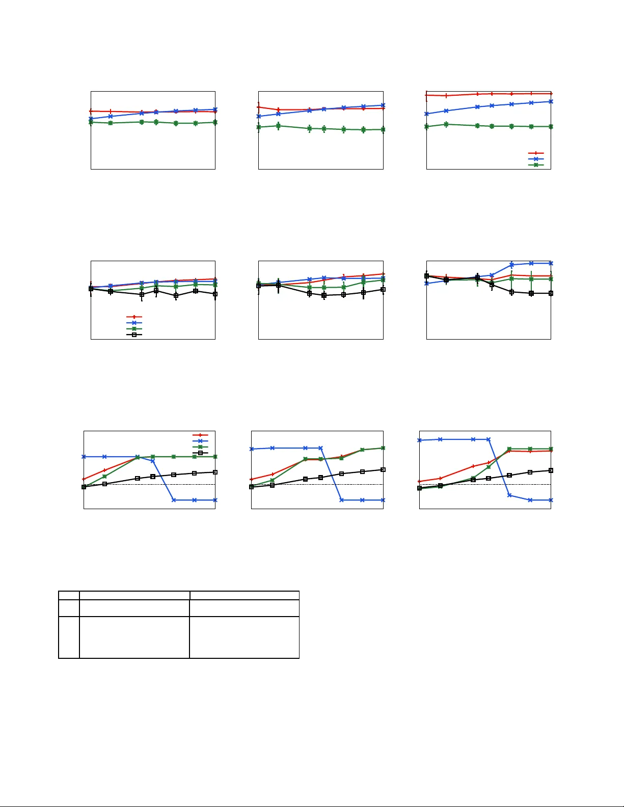
Learning Mark ov networks with context- specific indepen dences Alejandro Edera, Federico Schl ¨ uter , Facundo Bromberg Departamento de Sistemas de Informaci ´ on, Universidad T ecnol ´ ogica Nacional, F acultad Regional Mendoza , A r gentina. { aedera,federico .schluter ,fbr omber g } @frm.utn.edu.ar Abstract —Learning the Markov network structure from data is a problem that h as receiv ed considerable attention in machine learning, an d in many other appli cation fields. This work focuses on a p articular app roach for this pu rpose called independence-bas ed learning. Such app roach guarantees the learning of th e correct structure efficiently , when ev er data is sufficien t for representing th e underlying distribution. Howe ver , an imp ortant issue of su ch approach is that the learned structures are encoded in an und irected graph. The problem with graphs i s th at they cannot encode some types of independ ence relations, su ch as the context-specific ind epen- dences. They are a particular case of condition al independences that is tru e only fo r a certain assignment of its cond itioning set, in contrast to conditional ind ependences that mu st hold fo r all it s assignments. In this work we present CSPC, an independ ence-based algorithm fo r learning structures that encode context-specific ind ependences, and encoding them in a log -linear model, instead of a graph. The central id ea of CSPC is combinin g the th eoretical guarantees pro vided by th e independ ence-based approach with the benefits of repre senting complex structures by using features in a log-linear model. W e present experiments in a synthetic case, showing th at CS PC is more accurate than th e state-of-the-art IB algorithms when the underlying distribution contains CSIs. Key words -Marko v networks, structure learning; independ ence-based; context-specific ind ependences; I . I N T RO D U C T I O N Now adays, a powerful r epresentation of joint pro babil- ity distrib utions a re M arkov networks. T he structure of a Markov netw ork can enco de complex probab ilistic rela- tionships among the variables of the do main, imp roving the efficiency in th e proce dures for proba bilistic infer ence. An imp ortant problem is learn ing the structu re from sam- ples dr awn fr om an unknown distribution. A number of alternative algor ithms for this p urpose have bee n devel- oped in recent years. One appro ach is the indepen dence- based (I B) appr oach [1]–[5]. Alg orithms that follow this approa ch proceed by using statistical tests to learn a series of condition al ind ependen ces fro m data, enco ding them in an undirected gr aph. An important advantage of this approa ch is that it provid es theoretical g uarantees fo r learn ing the correct structure, together with the ef ficiency gained by using statistical te sts. Other recent a pproach es [6]–[9] pr oceed by inducing a set of features from data, instead o f an undirec ted graph. The f eatures are real- valued func tions of partial variable assignments, and using these fu nctions it is p ossible to en code mo re comp lex structures than tho se enco ded by graphs. Algor ithms that f ollow th is approach encod e th e structure in the features of a log- linear model. Unfortuna tely , current algorithm s based on learning features are not an efficient alternative, due to the multiple u ser d efined hy per- parameters, a nd th e need of p erform ing parameter s learning. The parameter s learnin g step is often intractable, requ iring an iterative optimization that runs an inferenc e step over th e model at each iteration. In many practical cases the under lying d istribution of a problem present co ntext-specific indep endenc es (CSIs) [10], that are conditiona l in depend ences that on ly h old for a certain assignment o f the conditioning set, but not h old for the r emaining assignm ents. In that case, encoding the structure in an und irected gr aph leads to excessi vely dense graphs, ob scuring the CSIs present in the distribution, a nd resulting in computation ally mo re expensive computatio n o f inference algorith ms [11], [12]. For this reason, encodin g the CSIs in a log -linear m odel does n ot o bscure th em, a chieving sparser mode ls and there fore significant improvemen ts in time, space and sample complexities [8], [ 13]–[15]. This work p resents CSPC, an indepe ndence- based algo- rithm f or lear ning a set o f featu res instead of a graph , in order to en code CSIs. The algorithm is design ed as an adaptation for this purp ose o f the well-k nown PC algo - rithm [16]. CSPC procee ds by first generating an in itial set of fe atures from the dataset, an d then searches over the space of possible contexts for learning the CSIs present in the und erlying d istribution. For ea ch context the algorith m elicits a set of CSIs u sing statistical tests, and g eneralizes the curr ent set of features in order to enco de the elicited CSIs. The centra l id ea of CSPC is co mbining the theo retical guaran tees provided by the in depend ence-based approa ch with the benefits of represen ting complex structures by using features. T o our knowledge, the only algorithm near to CSPC is the LEM algorith m [8], since it uses statistical tests to learn CSIs. However , LEM restricts the attention to lear n- ing distributions that can b e rep resented by decom posable Markov networks. For th e latter , we omit it as c ompetitor in our experiments. W e conduc ted an em pirical ev aluation o n sy nthetic data generated f rom kn own distributions that c ontains CSIs. In our experimen ts we p rove th at CSPC is significantly more accurate than the state-o f-the-ar t IB algorithms when the underly ing distribution co ntains CSIs. I I . B AC K G R O U N D This section reviews the basics about Markov ne tworks representatio n, the concept o f CSIs, an d the IB approach f or learning Markov networks. A. Markov networks A Mar kov network over a domain X o f n rando m variables X 0 . . . X n − 1 is r epresented by an undire cted graph G with n nod es and a set o f numerical parameters θ ∈ R . This representation can be u sed to factorize the distribution with the Hammersley-Clifford theor em [17], b y using the completely connected sub-graph s of G (a.k.a. , cliques ) into a set of potentia l functions { φ C ( X C ) : C ∈ cl i q ues ( G ) } of lower dime nsion th an p ( X ) , param eterized by θ , as f ollows: p ( X = x ) = 1 Z Y C ∈ cliques ( G ) φ C ( x C ) , (1) where x is a com plete assignmen t of the d omain X , x C is the projection of the assign ment x over the variables of the C th c lique, and Z is a no rmalization constant. An often used alternative repr esentation is a log-linear mo del, with each clique potential repr esented as an expon entiated weighted sum of features of the assignment, as follows: p ( X = x ) = 1 Z exp    X j θ j f j ( x )    , (2) where each fea ture f j is a par tial assignment over a subset of the dom ain V ( f j ) . Given an assignment x , a featur e f j is said to be satisfied iff f or each single variable X a = x a ∈ f j it also holds that x a ∈ x [ 8]. One ca n associate a in dicator function to f j and an assignment x b y associating a value 1 when f j is satisfied in x , or 0 otherwise. A Markov network can be induced fr om a log-linear model b y addin g an ed ge in the grap h between every p air of variables X a , X b that ap pear togeth er in some subset of a f eature f j , th at is { X a , X b } ⊆ V ( f j ) . Th en, the clique potentials ar e co nstructed fr om th e lo g-linear fea tures in the obvious way [18]. Example 1. F igur e 1 shows the featur es of a log- linear model over n = 3 binary variables X f , X a and X b , a nd its r espective induced g raph. B. Context-specific in depend ences The CSIs are a finer-grained type of i ndep endences. These indepen dences a re similar to conditio nal indepen dences, but hold for a spe cific assign ment of the co nditionin g set, called the con text of the independe nce. Formally , we define a CSI as follows: Definition 1 (Context-specific independ ence [ 10]) . Let X a , X b ∈ X be two random variab les, X U , X W ⊆ X \ f 1 ( X a = 0 X b = 0 X f = 0) f 2 ( X a = 1 X b = 0 X f = 0) f 3 ( X a = 0 X b = 1 X f = 0) f 4 ( X a = 1 X b = 1 X f = 0) f 5 ( X a = 0 X f = 1) f 6 ( X a = 1 X f = 1) f 7 ( X b = 0 X f = 1) f 8 ( X b = 1 X f = 1) ⇒ Figure 1 : An example of an in duced graph f rom a set of features. { X a , X b } b e pairwise disjoin t sets o f variables th at doe s not co ntain X a , X b ; an d x W some assign ment of X W . W e say that va riables X a and X b ar e contextually indepen dent given X U and a con text X W = x W , den oted I ( X a , X b | X U , x W ) , iff p ( X a | X b , X U , x W ) = p ( X a | X U , x W ) , (3) whenever p ( X b , X U , x W ) > 0 . Example 2. F igur e 2(a) shows the graph of Example 1, induced fr om a log- linear model. Notice that the featu r es of Example 1 enc ode the CSI I ( X a , X b | X f = 1) , but it is obscured in the graph. A lternatively , such CSI can be graphically repr esented if we use two g raphs, o ne for each value of X f . F or th is, F igur e 2( b) shows the g raph in duced fr om the features with X f = 1 which encod es I ( X a , X b | X f = 1) , and F igur e 2(c) shows the g raph ind uced fr om the featur es with X f = 0 which en codes ¬ I ( X a , X b | X f = 0) . In these figur es, gray nod es co rr espond to a n assignment of a variable. Figure 2: ( a) The g raph induced from the f eatures in Ex am- ple 1. (b) g raph ind uced from th e featu res with X f = 1 in Example 1. (c) graph induced from the features with X f = 0 in Examp le 1. Gray no des correspon d to an assignm ent of a variable. Notice that the graph in Figure 2(a) can not encode the C SI I ( X a , X b | X f = 1) , because it occu rs only for a sp ecific context an d is ab sent in all th e others. T his is b ecause the edg es conn ect p airs of variables tha t are c ondition ally depend ent even for a single ch oice of values of the other variables. Sinc e a CSI is de fined for a specific context, a set of CSIs cann ot be encoded all tog ether in a single un directed graph [19]. Noneth eless, b oth structures are enco ded in the set of feature s of the example. C. In depend ence-ba sed appr oach for structur e learning The task of IB algorithm s is learnin g a graph th at e ncodes the ind ependen ces fro m i.i.d . samples D = { x 1 , . . . , x D } of an unk nown un derlying distribution p ( X ) [1]. For that, these algorithm s perfo rm a succession of statistical ind ependen ce tests over D to determ ine th e truth value o f a con ditional indepen dence (e.g. Mutual I nform ation [20], Pearson ’ s χ 2 and G 2 [21]), discarding all g raphs th at are inco nsistent with the test. Th e dec ision o f wh at test to perfo rm is based on the indepen dences learned so far, and varying with ea ch sp ecific algorithm . A key advantage of these algorithm s is that they gu aran- tees to lear n the co rrect un derlying structure un der th ree as- sumptions: ( i ) the under lying distrib ution is graph-isomorph , that is, the in depend ences in p ( X ) can be en coded by a graph; ( ii ) the un derlying distribution is positive, tha t is p ( x ) > 0 f or all X = x ; and ( iii ) the outcomes of statistical indepen dence tests are c orrect, that is the ind ependen ces learned are a subset of th e indepen dences p resent in p ( X ) . Another ad vantage of u sing IB algorithms is its comp uta- tional efficiency , d ue to its po lynomial runn ing time [1], and also due to th e av o iding of the n eed of p erformin g parameters learning. The efficiency is gained be cause the computatio nal cost of a test is pr oportion al to the nu mber of rows in D , an d the numb er o f variables in volved in the tests. Perhaps the b est known a lgorithm that fo llows this ap - proach is PC [16], which was created for lear ning the structure o f Bayesian network s. PC is correct under the assumptions described above, but whe n the tests are not correct produ ce er rors in rem oving edge s, because the al- gorithm on ly tests for indepen dence among two variables condition ing in subsets of the ad jacencies of one of these variables. For lear ning M arkov networks, the first a lgorithm that follows the I B approach is GSMN [22], an ef ficient algorithm that comp utes only O ( n 2 ) tests, constructing the structure by lear ning the ad jacencies of each variable; using the Gr ow-Shrin k alg orithm [2 3]. A mo re rec ent algo rithm that improves over GSMN is IBMAP-HC [24], which learn s the struc ture b y p erformin g a hill-climb ing search over the space of grap hs looking for the on e which maxim izes the IB-score, a score o f the poster ior prob abilities of gr aphs p ( G | D ) . The h ill-climbing sear ch starts from th e emp ty structure, adding edg es until reaching a local max ima of p ( G | D ) . IBMAP-HC r elaxes the assumption abo ut the correctne ss of the statistical tests, im proving over GSMN in sample complexity by reducin g the cascade ef fect of incorrect tests. I I I . C O N T E X T - S P E C I FI C P A R E N T A N D C H I L D R E N A L G O R I T H M This section presents the CSPC (Con text-specific Par- ent and Children) algorith m for learning Markov networks structures that en codes the CSIs present in data. CSPC encodes the CSIs by generalizing iterati vely a set of features. For this, CSPC deco mposes the search space of CSIs in two n ested space s: the space of the p ossible co ntexts, and for each con text the space of all its possible CSIs. First, CSPC g enerates an initial set of features, and the n searche s over both spaces with two nested loops: an outer lo op that explores the space of the contexts; and for each one, an inner loop that elicits from data a set of CSIs by u sing statistical tests, and generalizes the featu res according to the elicited CSIs. The three key elements o f CSPC are: A) th e generatio n of the initial f eatures, B) the elicitation of CSIs from data, and C) the featur es g eneralization for encoding the elicited CSIs. A. The generation o f the initial featur es An initial set o f featur es F must be g enerated as a startin g point o f the whole alg orithm. One a lternative is to g enerate the features that c orrespon d with the initial fully connected graph in a similar fashion than PC, that is add ing a feature for each possible complete assignment x o f the variable X . In this case, the size o f such initial set is exp onential with respect to the numbe r o f variables. F o r this reason, CSPC u ses a more optimal initial set o f features, adding one feature for each u nique example in D . T his is an often used alternative [6] , [9], because it g uarantees that the genera lized features at the end of the algorithm match at least one training example. B. Eliciting con text-specific indepen dences For discovering all the CSIs pr esent in the data, CSPC explores th e set of complete con texts x found in th e dataset, that is, one for each uniq ue trainin g example. Given a context x ∈ D and a set o f feature s F , CSPC de cides what CSIs to elicit in a similar fashion than PC. For each variable X a a Markov network is indu ced fr om the subset of featur es that satisfies with the context x X \ X a . The n, for each X b adjacent to X a in the ind uced graph a sub set X W of the ad jacencies is taken in ord er to define the con ditional indepen dence I ( X a , X b | X W ) . From such indepen dence, a CSI is obtain ed by contextualizing the condition ing set X W using th e context x , that is I ( X a , X b | X W = x w ) . Fina lly , if th e CSI is presen t in d ata then it is encod ed in the current set of feature s. For eliciting the CSIs in d ata, we p ropose a straigh t- forward adap tation of a tradition al (non- contextualized) in - depend ence test. A similar adaptation is proposed in [8 ]. The centr al ide a of the adaptation is th at an arbitrary CSI I ( X a , X b | X U , x W ) ca n be seen as a conditio nal indepen dence I ( X a , X b | X U ) in the conditional distrib u tion p ( X \ { X W } | x W ) . In this way , the CSI can be tested b y us- ing a non-co ntextualized test over a sample drawn fro m the condition al distribution p ( X \ { X W } | x W ) . In p ractice, such sample can be obtained from D as { x j ∈ D : x j W = x W } , namely , the sub set of datapoints where X W = x W . C. F eatures generalization The generalization o f features is used by CSP C to en - code the CSIs that ar e present in data. A sp ecific CSI I ( X a , X b | x W ) can b e encoded in the features F o f a log- linear of p ( X ) by factorizing those features that correspo nd with the c ondition al d istribution p ( X \ { X W } | x W ) . Such factorization is done by using a recently pr oposed adaptation of the well known Hammer sley-Clif ford theo rem for CSIs called th e Context-Specific Hammersley-Clifford th eorem [25]. The featu res that correspo nd with p ( X \ { X W } | x W ) are the sub set of features in F that satisfy th e context x W , den oted by F [ x W ] ⊆ F . In this way , giv en the CSI I ( X a , X b | x W ) the fe atures F [ x W ] are factorized in to two ne w sets of features: F ′ [ x W ] , obtained from F [ x W ] but re moving th e variable X a ; and F ′′ [ x W ] , obtained fro m F [ x W ] but removin g th e variable X b . Formally , for all f ′ j ∈ F ′ [ x W ] , { X a } / ∈ V ( f ′ j ) ; and for a ll f ′′ j ∈ F ′′ [ x W ] , { X b } / ∈ V ( f ′′ j ) . Example 3 . F igure 3a sho ws a n initial set of featur e s F to be generalized in o r der to en code the CSI I ( X a , X b | X f = 1) . The gener alization co nsists in facto rizing th e featur es F [ X f = 1 ] , that is the set of fea tur es that ar e satisfied with the co ntext X f = 1 (Figur e 3 b). The factorization of these featur es results in two new sets o f fea tur e s: F ′ [ X f = 1] an d F ′′ [ X f = 1] , shown in F ig ur e 3c. The fea tur es in F ′ [ X f = 1] a r e ob tained fr om F [ X f = 1] but r em oving X b , and the features in F ′′ [ X f = 1] ar e obtained fr om F [ X f = 1] b ut r emoving X a F inally , the set of features which corr ectly encod es the CSI I ( X a , X b | X f = 1) ar e shown in F ig ur e 3 d. No tice that the fea tur es in F igure 3d ar e the same set o f featur es sho wn in Example 1. D. Overview This section pr esents an explanation of CSPC that pu ts all the p ieces togethe r . The pseudo code is shown in Algo- rithm 1. As inp ut, the algorithm receives the set of do main variables X , and a dataset D . Th e algo rithm starts by generating the initial set of fe atures. Th en, the space of the con texts is explor ed. For each co ntext, the curren t set of feature s is generalized by u sing a gener alization of the PC algorithm as a subroutin e. T his subro utine, described in Algo rithm 2, consists in th e elicitation o f CSIs and the featu res gen eralization steps. As inpu t, this subro utine receives the c urrent set o f features F , the co ntext x , the set of domain variables X , and the dataset D . At the end , the features of a log-linea r mod el are retu rned. In Algo rithm 2, the step of elicitation of CSIs follows the same strategy than PC, tr ying to find the indepen dences on the smallest n umber of variables in the conditionin g set. For this, the cond itioning set f or each variable X a consists on subset of size k o f the adjac encies a dj( a ) , terminating when f 1 ( X a = 0 X b = 0 X f = 0) f 2 ( X a = 1 X b = 0 X f = 0) f 3 ( X a = 0 X b = 1 X f = 0) f 4 ( X a = 1 X b = 1 X f = 0) f 5 ( X a = 0 X b = 0 X f = 1) f 6 ( X a = 1 X b = 0 X f = 1) f 7 ( X a = 0 X b = 1 X f = 1) f 8 ( X a = 1 X b = 1 X f = 1) (a) Initial set of features F [ X f = 1] = { f 5 ( X a = 0 X b = 0 X f = 1) , f 6 ( X a = 1 X b = 0 X f = 1) , f 7 ( X a = 0 X b = 1 X f = 1) , f 8 ( X a = 1 X b = 1 X f = 1) } (b) T he features that satisfy with the context X f = 1 F ′ [ X f = 1] = { f ′ 5 ( X b = 0 X f = 1) , f ′ 6 ( X b = 0 X f = 1) , f ′ 7 ( X b = 1 X f = 1) , f ′ 8 ( X b = 1 X f = 1) } F ′′ [ X f = 1] = { f ′′ 5 ( X a = 0 X f = 1) , f ′′ 6 ( X a = 1 X f = 1) , f ′′ 7 ( X a = 0 X f = 1) , f ′′ 8 ( X a = 1 X f = 1) } (c) Factorization of t he fea- tures F [ X f = 1] f 1 ( X a = 0 X b = 0 X f = 0) f 2 ( X a = 1 X b = 0 X f = 0) f 3 ( X a = 0 X b = 1 X f = 0) f 4 ( X a = 1 X b = 1 X f = 0) f ′ 5 ( X a = 0 X f = 1) f ′ 7 ( X a = 1 X f = 1) f ′′ 5 ( X b = 0 X f = 1) f ′′ 7 ( X b = 1 X f = 1) (d) Features generalized en- coding I ( X a , X b | x W ) Figure 3: Ex ample of f eature f actorization according to CSIs. Algorithm 1 : Context space explora tion Input : domain v ariables X , dataset D Output : features F generalized according to t he CSIs learned 1 F ← Generate one feature for each unique exa mple in D x ∈ V al( X ) 2 for each context x ∈ V al( X ) do 3 F ← PC ( F , x , X , D ) 4 Add atomic feature for each v ariable to F 5 return F for all subsets W , | W | is smaller th an k . This is a strategy fo r av oid ing the effect o f inco rrect tests, b ecause in the p ractice the qu ality o f statistical tests decreases expo nentially with the numb er of variables that ar e inv olved [2 1]. In Algor ithm 3 , the step o f features gener alization is made once the CSI has been elicited. In such step, fo r the input CSI I ( X a , X b | x W ) the current set o f features F is partitioned in two sets: the set F ′ that are the featur es tha t satisfy with x W , and the set F ′′ that are th e features that does not satisfy with x W . T hen, the satisfied features are factorized acco rding to the Con text-Specific Hammersley- Clif ford theorem. Finally , a new set of featu res F is defined by joining F ′ and F ′′ . I V . E X P E R I M E N TA L E V A L U A T I O N T o allo w a proper expe rimental design with a range o f well-under stood co nditions, we ev alu ated our appr oach on artificially generated datasets. For tes ting the ef fectiveness of our approa ch, we pro pose a specific class of deter ministic Algorithm 2 : PC extend ed fo r features Input : features F , conte xt x , domain variables X , dataset D Output : generalized features F 1 k ← 0 2 repeat 3 fo reach X a ∈ X do 4 adj( a ) ← compute adjacencies from features that satisfy x X \ X a 5 fo reach X b ∈ adj( a ) do 6 fo reach W subset of adj( a ) \{ X b } s.t. | W | = k do 7 if I ( X a , X b | x W ) is true t hen 8 F ← Generalize F for t he C SI I ( X a , X b | x W ) 9 k ← k + 1 10 unti l | adj( a ) \ { X b }| < k ; 11 return F Algorithm 3 : Feature generalization Input : features F , a CSI I ( X a , X b | x W ) Output : generalized features F 1 F ′ ← F [ x W ] 2 F ′′ ← F \ F ′ 3 F ′ ← factorize F ′ according to the C ontext-Specific Hammersley-Clif ford 4 return F ′ ∪ F ′′ models wh ich presents a controlled numb er of CSIs. The ev aluatio n co nsists in two parts. In the first part we sh ow the potential of impr ovements th at can be obtain ed in o ur experiment. In the second part we comp are CSPC to two state-of-the- art IB algor ithms: GSMN [22] and IBMAP-HC [24]. Additionally we also compar e w ith PC [1 6] in order to highlight the improvements resultin g from contextualizing it. Since PC was origin ally de signed for lear ning Bayesian networks (directed graphs), we use PC omitting the step of edges orientation [26]. A. Data sets W e g enerated artificial data th rough Gibb s samp ling on a class of m odels similar to Exam ple 2, generalized to distributions with n d iscrete binar y variables. W e c hose such models since they are a r epresentative c ase of a d istribution with a c ontrolled nu mber of CSIs. The aim is to d emonstrate that learning such C SIs represents an imp ortant improvement in the quality of learned distributions, wh en co mpared with the alter nativ e repr esentation in g raphs. I n th is scen ario, the IB algorithms lead to excessi vely d ense graphs (the fully co nnected ones), wh ich ob scures the u nderlyin g CSIs. W e consider ed mo dels with n ∈ { 6 , 7 , 8 } variables and maximum cliq ues of the same size. Since the comp lexity of structure learning grows expo nentially with the size o f its maximu m clique (a.k.a. treewidth), in the litera ture th e algorithm s are typically tested on models with maximum cliques of size at most 6 [8], [18]. For each n , the un derlyin g structu re is a fu lly co nnected graph with ( n − 1) nod es, plus a flag node X f . In this m odel, all pair s between the variables X \ { X f } are context-spec ific indepen dent, given the context X f = 1 . Instead, when X f = 0 the variables remain dep endent. In th is way , fo r n variables the u nderlyin g stru cture contain s ( n − 1) × ( n − 2) 2 contextual in depend ences in th e for m I ( X a , X b | X f = 1) , for all X a , X b 6 = X f ∈ X . Giv en such stru cture, we defined a lo g-linear model that contain s two sets of featu res: i) a set of pairwise featu res which encodes th e depe ndence between X f and the rest o f variables X \ { X f } , and ii) a set o f triplet features over the variables X a , X b , X f . For the resulting features we generated 10 dif f erent models, varying in its numerical pa rameters. Such parameters were generated to satisfy the log -odds ratio, in orde r to set strong depe ndencies in the model [3]–[5], [21]. In this way , th e parameter s of the pairwise features X a , X b were forced to satisfy the fo llowing ratio: ε = log  w 0 φ ( X a =0 ,X f =0) w 1 φ ( X a =1 ,X f =1) w 2 φ ( X a =0 ,X f =1) w 3 φ ( X a =1 ,X f =0)  , ∀ X a ∈ X \ { X f } , wh ere w 0 , w 2 are sym metric to w 1 , w 3 , respec - ti vely ( w 0 = w 1 and w 2 = w 3 ). Since this ratio has 2 unknowns we ch oose w 2 sampled from N (0 . 5; 0 . 001) , and w 0 is solved. Th e para meters for the triple t feature s were forced to satisfy th e CSI I ( X a , X b | X f = 1) . When X f = 0 the param eters we re generated using the sam e proced ure used for the pairwise features. When X f = 1 the parameters were forced to satisfy the following factorization : φ ( X a , X b , X f = 1) = w 0 φ ( X a = 0 , X f = 1) · w 1 φ ( X a = 1 , X f = 1) , where w 0 and w 1 are the same than the pairwise features alr eady d efined. In our experiments we set ε = 1 . 0 . The datasets were gene rated by samp ling from th e log-lin ear models using Rao-Blackwellized Gibbs sampler 1 with 10 chains, 100 burn-in and 100 0 samp ling. B. Metho dology W e used the synthetic datasets explained ab ove to learn the structu re and para meters for all th e algor ithms. Our syn- thetic data, to gether with an executable version of CSPC and the co mpetitors is pu blicly av ailable 2 . For a fair compa rison, we use Pearson’ s χ 2 as th e statistical indepen dent test for all the algorith ms, with a sign ificance level of α = 0 . 05 . The IBMAP-HC algorithm alternati vely o nly works by using the Bayesian test of Margaritis [23]. For each particu lar dataset we e valuated the algor ithms on trainin g set sizes varying fro m 500 to 4000 0 , in ord er to obtain a numb er of samples sufficient for satisfying the CSIs o f the un derlying distribution pro posed. W e r eport the quality of learned models using the Kullback-Leibler divergence ( KL ) [27]. T he KL is defined as K L ( p || q ) = P x p ( x ) ln p ( x ) q ( x ) , measuring the in formatio n 1 Gibbs sampler is ava ilable in the open-source Libra toolkit http:/ /libra.cs.uore gon.edu/ 2 http:/ /dharma.frm.utn.edu.ar/ papers/cspc lost when the lear ned d istribution q ( X ) is used to a pprox i- mate the un derlying d istribution p ( X ) . KL is equal to zero when p ( X ) = q ( X ) . The better th e learned models, the lower the values of th e KL measure. Since these algor ithms only learn the structure of a Markov n etwork, the complete distribution is obtained by lear ning its nu merical param eters. For the case of I B algo rithms, the features are induced fro m the maximum cliq ues o f the g raph learned. For learning its parameters w e co mputed th e pseudo- loglikelihood u sing the avail able version in the Lib ra toolkit. W e use p seudo- loglikelihood withou t regu larization to a void sparsity in the final mo del, because we are inte rested in measuring the quality of the structure learning step. C. Resu lts Our first experim ent sh ows the potential improvement th at can be obtain ed in our gener ated d atasets in terms o f KL over the g enerated d ata. For this we measure in Figure 4 the KLs obtained by learning th e parameters for three p ropo sed structures: i) the empty structure, ii) the f ully co nnected structure, an d iii) the un derlyin g structu re. The distribution learned from th e empty stru cture informs us about the im pact of en coding incor rect indepen dences in the KL measure. Consequently , the fully con nected structure sho ws the impact in the KL mea sure that can be obtaine d with incor rect depend ences that are ob scuring the real CSIs presen t in data. The u nderlyin g structure contains the features which exactly encodes the CS Is of th e p roposed mod el, as described in Section IV -A. The figure shows th e average and standard deviation over our 10 gen erated datasets for training set sizes varying from 50 0 to 4000 0 (X-axis), f or different do main sizes 6 , 7 an d 8 . In ord er to better show differences am ong the KLs we show it in log scale. In these results, we see empirically that the KL of the distribution obtain ed by learning th e p arameters for the un - derlying structur e is always significantly b etter than th e KL obtained by using th e em pty and fully structu res. Notice th at the KL is an ( expected) loga rithmic difference, representing differences in orders of magnitude in the no n-logar ithmic space. For our results, these differences a re up to 2 orders of ma gnitude in th e ca ses of n ∈ { 6 , 7 } , an d 5 order s o f magnitud e in the case of n = 8 . Howe ver , there is not a trend o f the KL to be zer o by varying the size of training data. Th is is b ecause Gibbs sam pler is not an exact method for th e gener ation of th e tra ining data. In this result also can be seen that as well as n increases, th e KL of th e fully structure is better than the KL of the empty structur e. In o ur second experimen t we compare the KLs obtained by CSPC, GSMN, IBMAP-HC, and PC. Th ese resu lts ar e shown in Figu re 5, f or the same datasets of the experim ent shown in Fig ure 4. CSPC is th e more accu rate algorithm in all the cases, with lo wer KL , near to 1 ( the KL value of the underlyin g structu re in Figure 4). Th e differences in KL between CSPC a gainst its co mpetitors is up to 2 o rders of magnitud e fo r n = 6 and n = 7 , and up to 5 order s o f magnitud e again st IBMAP-HC for n = 8 . Since the KL is clearly affected by the quality o f the structure, we wanted to determine whether or not their actual structures are co rrect. W e did th is by re porting the average feature leng th of the lear ned mode ls, since it is a k nown value for our u nderlyin g m odel in this experimen t. Th is is a statistical measure usefu l f or a nalyzing the structur al qu ality of log-lin ear mod els, as shown in several re cent work s [7], [9], [28 ]. Figure 6 re ports these values f or the same experiment shown above. Th e ho rizontal line in the g raphs shows the exact featu re length of the underly ing structure ( 2 . 80 fo r n = 6 , 2 . 83 for n = 7 , and 2 . 85 for n = 8 ). CSPC perfor m better in all the cases, showing always the neare st number of average featur e leng th to the horizo ntal line. This is consistent with the KL results shown in Figur e 5. GSMN and PC in creases in the average number of featur es length as well as the nu mber of datapo ints g rows, for all th e domain sizes. T his tren d is due because they are lea rning mor e dense structure s as well as the num ber of datapoin ts gr ows, reaching th e fully structure. For example, in the case o f n = 7 , th e GSMN and PC alg orithms shows a tren d to reach the fully structure, and th e KLs sho wn in Fig ure 5 are similar to the KL of the fu lly structure shown in Figure 4. Also, as well as n inc reases, the difference on the average featu re length between CSPC and its competitor s also increases. This is also con sistent with th e resu lts shown in Fig ure 4. A surprising r esult is sh own for IBMAP-HC, which does not show the same tr end than GSMN and PC. It can b e seen that for lower number of da tapoints ( D < 5 000 ) the algorithm learns fully stru ctures (the a verage f eature len gth is equa l to n in the th ree cases). Howev er, fo r higher num ber of datapoin ts ( D ≥ 500 0 ) the algorith m learns the empty structure, with av erage feature length eq ual to 1 ( the empty structure co ntains the ato mic features) . W e argue this is due to th e Bayesian nature of IBMAP-HC, which works by optimizing the po sterior p robability of structures p ( G | D ) with a hill-climb ing search. When using a large am ount of data, IBMAP-HC seems very pr one to g etting stuck in the empty structure as a local min ima with p ( G | D ) = 0 for almost all the structures, except the correct one with p ( G | D ) = 1 . Finally , as an additional re sult, we show in T a ble I the av erage featu re leng th of the featu res that are satisfied with the value of the flag variable X f . This result is shown for all the algorithms, run ning for an increasing numb er of variables f rom n = 4 to 8 wit h a fixed n umber of 3000 datapoints, and discriminating in d ifferent columns the value of X f . As expected , the values for CSPC for X f = 0 are more near to 3 , and mor e near to 2 for X f = 1 , in compariso n with the rest of the competito rs. In summary , the above results sup port ou r th eoretical claims and demon strate the efficiency of CSPC f or learning distributions with CSIs. 0.1 1 3 6 1000 10000 Kullback-Leibler divergence Number of datapoints n=6 0.1 1 3 6 1000 10000 Kullback-Leibler divergence Number of datapoints n=7 0.1 1 3 6 1000 10000 Kullback-Leibler divergence Number of datapoints n=8 EMPTY FULLY UNDERLYING Figure 4 : Po tential improvements in KL obtaine d by learning parameter s for the un derlying structur e, the fu lly and th e empty structures. A verage an d standard deviation over ten re petitions for increasing number of datapo ints in th e training set for domain sizes 6 (left), 7 (center) and 8 (righ t). 0.1 1 3 6 1000 10000 Kullback-Leibler divergence Number of datapoints n=6 GSMN IBMAP-HC PC CSPC 0.1 1 3 6 1000 10000 Kullback-Leibler divergence Number of datapoints n=7 0.1 1 3 6 1000 10000 Kullback-Leibler divergence Number of datapoints n=8 Figure 5: Comp arison o f KLs ob tained by learn ing para meters f or CSPC, GSMN, IBMAP-HC and PC. A verage and stan dard deviation over ten repe titions for increa sing number of d atapoints in the train ing set for domain sizes 6 (lef t), 7 (center) and 8 (righ t). 0 1 2 3 4 5 6 7 8 9 1000 10000 Length of features Number of datapoints n=6 GSMN IBMAP-HC PC CSPC 0 1 2 3 4 5 6 7 8 9 1000 10000 Length of features Number of datapoints n=7 0 1 2 3 4 5 6 7 8 9 1000 10000 Length of features Number of datapoints n=8 Figure 6: Compa rison of the average f eature length ob tained for CSPC, GSMN, IBMAP- HC and PC. A verage and standard deviation over ten repe titions for increa sing number of d atapoints in the train ing set for domain sizes 6 (lef t), 7 (center) and 8 (righ t). The average feature length of the solution under lying structu re is th e horizo ntal line. X f = 0 X f = 1 n GSMN IBMAP- HC PC CPSC GSMN IBMAP- HC PC CPSC 4.00 4.00 4.00 4.00 4.00 4.00 4.00 4.00 1.85 5.00 5.00 4.60 5.00 4.79 5.00 4.60 5.00 1.88 6.00 6.00 5.50 6.00 4.37 6.00 5.50 6.00 1.93 7.00 5.00 7.00 1.10 4.01 5.00 7.00 1.10 1.95 8.00 3.00 8.00 1.00 3.54 3.70 8.00 1.00 1.87 T ab le I: Num ber of features learn ed f or increasing n , and using D = 3 000 . V . C O N C L U S I O N S This paper prop osed CSP C, an ind epende nce-based al- gorithm f or lear ning a set of fea tures, instead of a graph. CSPC overcomes some of the inefficiency o f traditional IB algor ithms by learning CSIs from data and repr esenting them in a log -linear model. CSPC pr oceeds by gener alizing iterativ ely a set o f in itial featur es in order to re present the CSIs pr esent in data, e xplor ing the possible c ontexts, eliciting fro m data a set of CSIs usings statistical tests, and generalizing the features accord ing to the elicited CSIs. Experime nts in a synthetic case show that this approach is more accurate than the state-of-the-ar t IB algo rithms, wh en the un derlyin g distribution contains CSIs. Directions o f fu- ture work inc lude: adaptin g more efficient IB algo rithms for learning CSIs; validation in real world datasets; comparison against state-of- the-art non-ind epende nce-based ap proach es [6]–[9]; a dding Mo ore and Lee’ s AD-trees [ 29] for speeding up the execution of statistical tests, etc. R E F E R E N C E S [1] P . S pirtes, C. Glymour , and R. S cheines, Causation, P r edic- tion, and Sear ch , ser . Adaptiv e Computation and Mach ine Learning Series. MIT Press, 2000. [2] F . Bromberg, D. Margaritis, and H. V ., “Efficient Marko v Network S tructure Discovery Using Indepen dence T ests, ” J AIR , v ol. 35, pp. 449–48 5, July 2009. [3] P . Gandhi, F . Bromb erg, and D. Mar gariti s, “Learning Mark ov Network Structure using Few Independen ce T ests, ” in SIAM International Confer ence on Da ta Mining , 20 08, pp. 680– 691. [4] D. Margaritis and F . Bromberg, “Efficient Markov Network Discov ery Using Particle Fil ter, ” C omp. Intel. , vol. 25, no. 4, pp. 367–394 , 2009. [5] F . Bromber g, F . Schl ¨ uter, and A. Edera, “Independe nce- based MAP for Marko v networks structure disco very , ” in International C onfer ence on T ools with Artificial Intelligence , 2011, http://ai.frm.utn.edu.ar/fschluter/p/11d.pdf. [6] J. D avis and P . Domingos, “Bottom-up learning of markov network str ucture, ” in Proceed ings of the 27th International Confer ence on Machine Learning , 2010, pp. 271–280 . [7] D. L o wd and J. Davis, “Learning markov network str ucture with decision trees, ” in Data Min ing (ICDM), 2010 IEEE 10th International Confer ence on . IEEE , 2010 , pp. 334–343. [8] V . Gogate, W . W ebb, and P . Domingos, “Learning ef ficient marko v networks, ” in Advances in Neural Information P r o- cessing Systems , 2010, pp. 748–756. [9] J. V an Haaren and J. Davis, “Marko v network structure learning: A randomized feature generation approach, ” in Pr oceedings of the T wenty-Sixth National Confer ence on Artificial Intelligence . AAAI Pr ess , 2012. [10] C. Boutilier, N. Fri edman, M. Goldsz midt, and D. Koller , “Context-sp ecific independence in Bayesian networks, ” i n Pr oceedings of the T welfth internationa l confer ence on Uncer- tainty in artificial intelligence . Morgan Ka ufmann Publishers Inc., 1996, pp. 115–12 3. [11] D. Poole and N. L. Z hang, “Exploiting contextual indepen - dence in probabilistic inference, ” J. Artif. Intell. Res.(J AIR) , vol. 18, pp. 263–313, 2003. [12] A. Fridman, “Mixed mark ov models, ” Pr oceedings of the National Academy of Sciences , vol. 100, no. 14, pp. 8092– 8096, 2003. [13] C. Benedek and T . Szir ´ anyi, “ A mixed marko v model for change detection in aerial photos w ith large time differences, ” in P attern R ecog nition, 2008. ICP R 2008. 19th International Confer ence on . IE EE, 2008, pp. 1–4. [14] D. Fierens, “Context-spe cific independen ce in directed rela- tional probabilistic models and its influence on t he efficienc y of Gibbs sampling, ” in Eur opean Confer ence on A rtificial Intelligence , 2010 , pp. 243–248. [15] Y . W e xler an d C. Meek, “Inference for mu ltiplicative models, ” in Uncertainty in Artificial Intell igence , 2008, pp. 595– 602. [16] P . Spirt es and C. Glymour , “ An algorithm for fast recovery of sparse causal graphs, ” Social Science Computer Review , vol. 9, no. 1, pp. 62–72, 1991. [17] J. M. Hammersley and P . Clifford , “Markov fields on finite graphs and lattices, ” 1971 . [18] S. Lee, V . Ganapathi, and D. Koller , “Efficient structure learning of Markov networks using L1-regularization, ” in Neural Information P r ocessing Systems . Citeseer, 2006. [19] D. K oller and N. Fr iedman, Prob abilistic G raph ical Models: Principles and T ec hniques . MIT Press, Cambridge, 2009. [20] T . M. Cov er and J. A. Thomas, Elements of information theory . Ne w Y ork, NY , USA: W iley-Interscience, 1991. [21] A. Agresti, C ate gorical Data Analysis , 2nd ed. Wile y , 2002. [22] F . Bromberg, D. Margaritis, V . Honav ar et al. , “Efficient marko v network structure discovery using i ndepend ence tests, ” J ournal of Artificial Intellig ence Resear ch , v ol. 35, no. 2, p. 449, 2009. [23] D. Margaritis and S. Thrun, “Bayesian network induction via local neighbo rhoods, ” DTI C Document, T ech. Rep., 2000. [24] F . Bromberg, F . Schluter , and A. Edera, “Independence-ba sed map f or mark ov netwo rks structure discovery , ” in T ools with Artificial Intelligence (ICT AI), 2011 23r d IEE E International Confer ence on . IE EE, 2011, pp. 497–504. [25] A. Edera, F . B romberg , and F . S chl ¨ uter, “Marko v ran- dom fields factorization with context-specific independences, ” arXiv pr eprint arXiv:1306.2295 , 2013. [26] M. Kalisch and P . B ¨ uhlmann, “Estimating high-dimensional directed acyclic graphs with the pc-algorithm, ” The Journa l of Mac hine Learning Resear ch , vol. 8, pp. 613–636 , 2007. [27] S. Kullback and R. A. Leibler , “On i nformation and suffi- ciency , ” The Annals of Mathematical Statistics , vol. 22, no. 1, pp. 79–86, 1951. [28] D. Lo wd and A. Rooshenas, “Learning marko v networks with arithmetic circuits, ” The Journal of Mac hine Learning Resear ch , vol. 31, pp. 406–414, 2013. [29] A. Moore and M. S. Lee, “Cached suficient statistics for e cient machine learning with large datasets, ” J ournal of Artificial Intelligence R esear ch , vol. 8, pp. 67–91, 1998.