A Note on Probabilistic Models over Strings: the Linear Algebra Approach

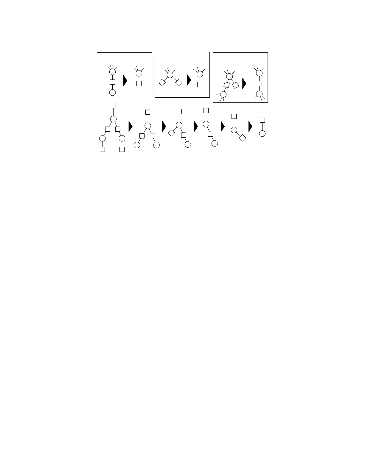
A Note on Probabilistic Mo dels o v er Strings: the Linear Algebra Approac h Alexandre Bouc hard-Cˆ ot ´ e No vem ber 1, 2018 Abstract Probabilistic mo dels ov er strings hav e pla yed a k ey role in developing metho ds allowing indels to be treated as ph ylogenetically informative ev en ts. There is an extensiv e literature on using automata and transducers on phylogenies to do inference on these probabilistic models, in which an imp ortant theoretical question in the field is the complexity of computing the normalization of a class of string-v alued graphical models. This question has b een in v estigated using to ols from combinatorics, dynamic programming, and graph theory , and has practical applications in Ba yesian ph ylogenetics. In this work, we revisit this theoretical question from a differen t p oin t of view, based on linear algebra. The main con tribution is a new pro of of a known result on the complexit y of inference on TKF91, a well-kno wn probabilistic mo del o ver strings. Our pro of uses a differen t approach based on classical linear algebra results, and is in some cases easier to extend to other mo dels. The proving method also has consequences on the implementation and complexit y of inference algorithms. k eywords indel, alignment, probabilistic models, TKF91, string transducers, automata, graphical mo dels, ph ylogenetics, factor graphs 1 In tro duction This w ork is motiv ated by models of evolution that go beyond substitutions by incorp orating insertions and deletions as phylogenetically informative ev ents [46, 47, 33, 32, 6]. In recent y ears, there has b een significan t progress in turning these models in to phylogenetic reconstruction metho ds that do not assume that the sequences ha ve b een aligned as a pre-pro cessing step, and into statistical alignment metho ds [15, 30, 31, 26, 38, 40, 39, 3]. Join t ph ylogenetic reconstruction and alignment methods are app ealing b ecause they can pro duce calibrated confidence assessmen ts [40], they lev erage more information than pure substitution models [25], and they are generally less susceptible to biases induced by conditioning on a single alignment [52]. Mo del-based joint ph ylogenetic metho ds require scoring eac h tree in a large collection of h yp oth- esized trees [38]. This collection of prop osed trees is generated b y a Marko v chain Monte Carlo (MCMC) algorithm in Ba yesian metho ds, or by a searc h algorithm in frequen tist metho ds. Scoring one hypothesized tree then b oils down to computing the probability of the obse rv ed sequences given the tree. This computation requires summing ov er all possible ancestral sequences and deriv ations (a refinement of the notion of alignment, lo calizing all the insertions, deletions and substitutions on the fixed tree that can yield the observed sequences) [21]. Since the length of the ancestral strings is a priori unkno wn, these summations range ov er a coun tably infinite space, creating a c hallenging problem. This situation is in sharp con trast to the classical setup where an alignment is fixed, in whic h case computing the probability of the observed aligned sequences can b e done efficiently using the standard F elsenstein recursion [12]. When an alignmen t is not fixed, the distribution o ver a single branc h is typically expressed as a transducer [15], and the distribution ov er a tree is obtained by comp osite transducers and automata 1 [21]. The idea of comp osite transducers and automata, and their use in ph ylogenetic, ha ve b een in- tro duced and subsequently developed in previous work in the framework of graph representations of transducers and com binatorial methods [21, 16, 17, 18, 28, 9]. Our con tribution lies in new proofs, and a theoretical approach purely based on linear algebra. W e use this linear algebra formulation to obtain simple algebraic expressions for marginalization algorithms. In the general cases, our representation pro vides a slight improv ement on the asymptotic worst-case running time of existing transducer algo- rithms [36]. W e also characterize a sub class of problems, which we call triangular pr oblems , where the running time can b e further impro ved. W e show, for example, that marginalization problems derived from the p opular TKF91 [46] are triangular. W e use this to dev elop a new complexity analysis of the problem of inference in TKF91 mo dels. The b ounds for TKF91 on star trees and p erfect trees coincide with those obtained from previous w ork [29], but our proving metho d is easier to extend to other models since it only relies on the triangularit y assumption rather than on the details of the TKF91 mo del. Algorithms for composite phylogenetic automata and transducers ha v e b een in tro duced in [21, 19], generalizing the dynamic programming algorithm of [16] to arbitrary guide trees. Other related work based on combinatorics includes [44, 29, 43, 41, 4]. See [7] for an outline of the area, and [20, 38, 37] for computer implemen tations. Our w ork is most closely related to [48, 49], whic h extends F elsenstein’s algorithm to transducers and automata. They use a differen t view based on partial-order graphs to represen t ensem ble profiles of ancestral sequences. While the exact metho ds describ ed here and in previous w ork are exponential in the num b er of taxa, they can form the basis of efficient appro ximation methods, for example via existing Gibbs sampling methods [23, 38]. These methods augment the state space of the MCMC algorithm, for example with internal sequences. The running time then dep ends on the n umber of taxa inv olved in the lo cal tree perturbation. This n umber can b e as small as tw o, but there is a trade-off b et ween the mixing rate of the MCMC c hain and the computational cost of eac h mo ve. Note that the matrices used in this w ork should not b e confused with the rate matrices and their marginal transition probabilities. The latter are used in classical ph ylogenetic reconstruction setups where the alignment is assumed to b e fixed. Our proving methods are more closely related to previous work on representation of sto c hastic automata netw ork [13, 27], where interactions represent sync hronization steps rather than string evolution, and therefore b ehav e differently . 2 F ormal description of the problem 2.1 Notation W e use τ to denote a rooted ph ylogeny , with top ology ( V , E ). 1 The ro ot of τ is denoted b y Ω; the paren t of v ∈ V , v 6 = Ω, b y pa( v ) ∈ V ; the branch lengths b y b ( v ) = b (pa( v ) → v ); and the set of lea ves b y L ⊂ V . The mo dels w e are interested in are tree-shap ed graphical mo dels [24, 2, 1] where no des are string- v alued random v ariables X v o ver a finite alphab et Σ (for example a set of nucleotides or amino acids). There is one suc h random v ariable for each no de in the topology of the ph ylogeny , v ∈ V , and the v ariable X v can b e interpreted as an hypothesized biological sequence at one p oin t in the phylogen y . Eac h edge (pa( v ) → v ) denotes ev olution from one species to another, and is asso ciated with a conditional probability P τ ( X v = s 0 | X pa( v ) = s ) = θ v ( s, s 0 ), where s, s 0 ∈ Σ ∗ are strings (finite sequences of characters from Σ). These conditional probabilities can b e deriv ed from the marginals of contin uous time sto c hastic pro cess [46, 21, 33, 32], or from a parametric family [26, 40, 38, 39]. W e also denote the distribution at the ro ot by P τ ( X Ω = s ) = θ ( s ), whic h is generally set to the stationary distribution in rev ersible mo dels or to some arbitrary initial distribution otherwise. Usually , only the sequences at the terminal no des are observed, an even t that w e denote by Y = ( X v = x v : v ∈ L ). 1 In reversible models such as TKF91, an arbitrary ro ot can b e selected without changing the likelihoo d. In this case, the ro ot is used for computational con venience and has no special phylogenetic meaning. 2 root / MCRA modern species Figure 1: F actor graph construction (right) derived from a phylogenetic tree (left): in green, the unary factor at the ro ot capturing the initial string distribution; in blue, the binary factors capturing string m utation probabilities; and in red, the unary factor at the leav es, whic h are indicator functions on the observed strings. W e denote the probabilit y of the data giv en a tree b y P τ ( Y ). The computational bottleneck of mo del-based metho ds is to rep eatedly compute P τ ( Y ) for different hypothesized phylogenies τ . This is the case not only in maxim um likelihoo d estimators, but also in Bay esian metho ds, where a ratio of the form P τ 0 ( Y ) / P τ ( Y ) is the main contribution to the Metrop olis-Hastings ratio driving Marko v Chain Monte Carlo (MCMC) approximations. While it is more intuitiv e to describ e a ph ylogenetic tree using a Ba yesian netw ork, it is useful when dev eloping inference algorithms to transform these Ba yesian net works in to equiv alen t factor graphs [2]. A factor graph enco des a weigh t function ov er a space X assumed to b e countable in this work. F or example, this weigh t function could b e a probabilit y distribution, but it is conv enient to drop the requiremen t that it sums to one. In phylogenetics, the space X is a tuple of | V | strings, X = (Σ ∗ ) | V | . A factor graph (see Figure 1 for an example) is based on a sp ecific bipartite graph, built by letting the first bipartite comp onen t correspond to V (the nodes denoted b y circles in the figure), and the second bipartite comp onen t, to a set of p otentials or factors W describ ed shortly (the no des denoted b y squares in the figure). W e put an edge in the factor graph b etw een w ∈ W and v ∈ V if the v alue taken b y w depends on the string at no de v . F ormally , a p otential w ∈ W is a map taking elemen ts of the pro duct space, ( x v : v ∈ V ) ∈ X , and returning a non-negative real num b er. How ev er the v alue of the factors we consider only dep end on a small subset of the v ariables at a time. More precisely , w e will use t wo t yp es of factors: unary factors, whic h dep end on a single v ariable, and binary factors, which dep end on tw o v ariables. W e use the abbreviation SFG for such string-v alued factor graph. In order to write a precise expression for the probability of the data giv en a tree, P τ ( Y ), we con- struct a factor graph (sho wn in Figure 1) with three types of factors: one unary potential w Ω ( s ) = θ ( s ) at the root mo deling the initial string distribution; binary factors w v ,v 0 ( s, s 0 ) = θ v 0 ( s, s 0 ) capturing string mutation probabilities b et ween pairs of sp ecies connected by an edge ( v → v 0 ) in the phyloge- netic tree; and finally , unary factors w v ( s ) = 1 [ s = x v ] attached to each leaf v ∈ L , which are Dirac deltas on the observed strings. F rom this factor graph, the likelihoo d can b e written as: P τ ( Y ) = X ( s v ∈ Σ ∗ : v ∈ V ) ∈ (Σ ∗ ) | V | w Ω ( s Ω ) Y v ∈ L w v ( s v ) !   Y ( v → v 0 ) ∈ E w v ,v 0 ( s v , s v 0 )   . F or an y functions f i : X i → R + o ver a coun table spaces X , we let Q i f i denote their p oin twise pro duct, and we let k f k denote the sum of the function o ver the space, k f k = X x ∈X f ( x ) . 3 The likelihoo d can then b e expressed as follows: P τ ( Y ) =      Y w ∈ W w      , (1) So far, we ha ve seen each potential w as a black b o x, fo cussing instead on how they interact with eac h other. In the next section, we describ e the form assumed by each individual p oten tial. 2.2 W eighted automata and transducers W eighted automaton (respectively , transducers), is a classical w ay to define a function from the space of strings (resp ectiv ely , the space of pairs of strings) to the non-negativ e reals [42]. A t a high lev el, w eighted automata and transducers pro ceed b y extending a simpler w eight function defined ov er a finite state space Q into a function o ver the space of strings. This is done via a collection of paths (lists of v ariable length) in Q . W e explain how this is done, starting with automata (in the language of SFG, unary p oten tials). First, w e designate one state in the state space Q to be the start state and one to b e the end state (w e need only consider one of each without loss of generality). W e define a p ath as a sequence of states q i ∈ Q and emissions ˆ σ i ∈ ˆ Σ = Σ ∪ {  } , starting at the start state and ending at the stop state: p = ( q 0 , ˆ σ 1 , q 1 , ˆ σ 2 , q 2 , . . . , ˆ σ n , q n ). Here the set of p ossible emissions ˆ Σ is the set of c haracters extended with the empty emission  . 2 Let us now assign a non-negativ e num b er to eac h triplet formed b y a transition (pair of state q , q 0 ∈ Q ) and emission ˆ σ ∈ ˆ Σ. 3 W e call this map w : ˆ Σ × Q 2 → [0 , ∞ ), a parameter sp ecified by the user. 4 Next, we extend the input space of w in tw o steps. First, if w takes a path p as input, we define w ( p ) as the pro duct of the weigh ts of the consecutiv e triplets ( q i , ˆ σ i +1 , q i +1 ) in p . Second, if w takes a string s ∈ Σ ∗ as input, we define w ( s ) as the sum of the weigh ts of the paths p emitting s , where a path p emits a string s if the list of c haracters in p , omitting  , is equal to s . F or transducers (binary potentials), we mo dify the abov e definition as follows. First, emissions b ecome pairs of symbols in ˆ Σ × ˆ Σ. Second, paths are similarly extended to emit pairs of symbols at eac h transition, p = ( q 0 , ( ˆ σ 1 , ˆ σ 0 1 ) , q 1 , ( ˆ σ 2 , ˆ σ 0 2 ) , q 2 , . . . , ( ˆ σ n , ˆ σ 0 n ) , q n ). Finally a path emits a pair of strings ( s, s 0 ) if the concatenation of the first c haracters of the emissions, ˆ σ 1 , ˆ σ 2 , . . . , ˆ σ n , is equal to s after remo ving the  symbols, and similarly for s 0 with the second characters of eac h emission, ˆ σ 0 1 , ˆ σ 0 2 , . . . , ˆ σ 0 n . F or example, p = ( q 0 , (a ,  ) , q 1 , (b , c) , q 2 , ( ,  ) , q n ) emits the pair of strings (ab, c). The normalization of a transducer or automata is the sum of all the v alid paths’ w eights, Z = k w k . W e set the normalization to p ositiv e infinity when the sum diverges. W e now hav e reviewed all the ingredients required to formalize the problem we are interested in: Problem description: Computing Equation (1), where eac h w ∈ W is a w eighted automaton or transducer organized into a tree-shap ed SFG. 3 Bac kground In the previous section, w e ha v e shown how the normalization of a single factor is defined (ho w to compute it in practice is a another issue, that we address in Section 5). In this section, we review how to transform the problem of computing the normalization of a full factor graph, Equation (1), in to the problem of finding the normalization of a single unary factor. This is done using the elimination 2 Note that we use the conv ention of using ˆ σ when the character is an element of the extended set of characters ˆ Σ. 3 In technical terms, we use the Mealy mo del. 4 The inv erse problem, learning the values for this map is also of in terest [22], but here we fo cus on the forw ard problem. 4 ... ... M M (m) (a) Marginalization ... M (1) M (2) ... M (p) (b) Pointwise product (first kind) ... M (1) M (2) ... ... ... M (p) (c) Pointwise product (second kind) (b) (a) (b) (a) (c) Figure 2: T op: The tree graph transformations used in the elimination algorithm. Bottom: An example of the application of these three op erations on a graph induced by a ph ylogenetic tree. algorithm [2], a classical metho d used to break complex computations on graphical mo dels in to a sequence of simpler ones. The elimination algorithm is t ypically applied to find the normalization of factor graphs with finite- v alued or Gaussian factors. Since our factors tak e v alues in a different space, the space of strings, it is useful in this section to tak e a different p erspective on the elimination algorithm: instead of viewing the algorithm as exc hanging messages on the factor graph, we view it as applying transformation on the top ology of the graph. These op erations alter the normalization of individual p oten tials, but, as w e will show, they k eep the normalization of the whole factor graph inv ariant, just as in standard applications of the elimination algorithm. The elimination algorithm starts with the initial factor graph, and eliminates one leaf no de at eac h step (either a v ariable no de or a factor node, there must b e at least one of the tw o t yp es). This pro cess creates a sequence of factor graphs with one less no des at each step, un til there are only tw o nodes left (one v ariable and one unary factor). While the individual factors are altered b y this pro cess, the global normalization of each intermediate factor graph remains unchanged. W e show in Figure 2 an example of this pro cess, and a classification of the op erations used to simplify the factor graph. W e call the op erations corresp onding to a factor eliminations a p ointwise pr o duct (Figure 2(b,c)), and the op erations corresp onding to v ariable eliminations, mar ginalization (Figure 2(a)). W e further define tw o kinds of p oin twise pro ducts: those where the v ariable connected to the eliminated factor is also connected to a binary factor (the first kind, sho wn in Figure 2(b)), and the others (second kind, sho wn in Figure 2(c)). Let W denote a set of factors, and let W 0 denote a new set of factors obtained b y applying one of the three op erations describ ed abov e. F or the elimination algorithm to b e correct, the following in v ariant should hold [2]:      Y w ∈ W w      =      Y w 0 ∈ W 0 w 0      . 4 Indexed matrices In this section, we describ e the representation that forms the basis of our normalization metho d and establish the main prop erties of this representation. W e use TKF91 [46] as a running example to illustrate the construction. 5 a: p b: q ε :1- q-p M a =  p 0 0 0  M b =  q 0 0 0  M  =  0 1 − p − q 0 0  Figure 3: An initial geometric length distribution unary factor. On the left, w e show the standard graph-based automaton represen tation, where states are dashed circles (to differen tiate them from no des in SFGs), and arcs are lab elled by emissions and w eights. Zero w eight arcs are omitted. The start and stop state are indicated b y inw ard and outw ard arrows, resp ectiv ely on the first and second state here. On the right, w e sho w the indexed matrix represen tation of the same unary p oten tial. a:1 b:1 a:1 M a =     0 1 0 0 0 0 0 0 0 0 0 1 0 0 0 0     M b =     0 0 0 0 0 0 1 0 0 0 0 0 0 0 0 0     M  = 0 Figure 4: A unary factor enco ding a string indicator function. In this example, only the string ‘aba’ is accepted (i.e. the string ‘aba’ is the only string emitted with p ositiv e weigh t). 4.1 Unary factors W e assume without loss of generalit y that the states of the automata are labelled by the integers 1 , . . . , K , and that state 1 is the start state, and K , the stop state. W e represen t an automaton as a character-indexed collection, M , of K × K matrices, where K is the size of the state space of the automaton, and the index runs ov er the extended c haracters: M =  M ˆ σ ∈ M K  R +   ˆ σ ∈ ˆ Σ Eac h en try M ˆ σ ( k , k 0 ) enco des the weigh t of transitioning from states k to k 0 while emitting ˆ σ ∈ ˆ Σ. An indexed collection M sp ecifies a corresponding w eight function w M : Σ ∗ → [0 , ∞ ) as follows: let p denote a v alid path, p = q 0 , ˆ σ 1 , q 1 , ˆ σ 2 , q 2 , . . . , ˆ σ n , q n , and set w M ( p ) = φ n Y i M ˆ σ i ! , where φ selects the en try (1 , K ) corresp onding to the pro duct of weigh ts starting from the initial and ending in the final state, φ ( M ) = M (1 , K ). The pro duct denotes a matrix multiplication ov er the matrices indexed by the emissions in p , in the order of o ccurrence. In the TKF91 model for example, an automaton is needed to mo del the geometric ro ot distribution, θ ( s ). W e ha ve in Figure 3 the classical state diagram as w ell as the indexed matrix represen tation, in the case where the length distribution has mean 1 / (1 − q − p ), and the prop ortion of ‘a’ symbols v ersus ‘b’ symbols is p/q . Another imp ortan t example of an automaton is one that gives a weigh t of one to a single observed string, and zero otherwise: w v ( s ) = 1 [ s = x v ]. W e sho w the state diagram and the indexed matrix represen tation in Figure 4. Note that the indexed matrices are triangular in this case, a prop ert y that will hav e imp ortan t computational consequence in Section 6. 6 ( σ , σ ' ) ( ε , σ ) ( ε , σ ) ( σ , σ ' ) ( σ , ε ) ( σ , ε ) M σ,σ 0 = αλ µ  (1 − β ) 0 (1 − γ ) 0  P σ,σ 0 M σ, = λ (1 − α ) µ  0 (1 − β ) 0 (1 − γ )  M ,σ = π σ  β 0 γ 0  Figure 5: A binary factor enco ding a TKF91 marginal. 4.2 Binary factors W e now turn to the w eighted transducers, whic h we view ed as a collection of matrices as well, but this time with an index running ov er pairs of symbols ( ˆ σ , ˆ σ 0 ) ∈ ˆ Σ: M =  M ˆ σ , ˆ σ 0 ∈ M K  R +   ˆ σ , ˆ σ 0 ∈ ˆ Σ Note that in the con text of transducers, epsilons need to b e k ept in the basic represen tation, otherwise transducers could not give p ositive weigh ts to pairs of strings where the input has a differen t length than the output. In ph ylogenetics, transducers represent the key comp onen t of the probabilistic model: the prob- abilit y of a string giv en its paren t, w v ,v 0 ( s, s 0 ) = θ v 0 ( s, s 0 ). F or example, in TKF91 mo dels, this probabilit y is determined b y three parameters: an insertion rate λ > 0, a deletion rate µ > 0, and a substitution rate matrix Q . Given a branc h of length t , the probabilit y of all deriv ations b et w een s and s 0 can b e marginalized using the transducer shown in Figure 5, where the v alues of α , β and P are obtained by solving a system of differential equations yielding [46], for all σ, σ 0 ∈ Σ: α ( t ) = exp( − µt ) β ( t ) = λ (1 − exp(( λ − µ ) t )) µ − λ exp(( λ − µ ) t ) γ ( t ) = 1 − µβ ( t ) λ (1 − α ( t )) P t ( σ, σ 0 ) =  exp( tQ )  ( σ, σ 0 ) , and π σ is the stationary distribution of the process with rate matrix Q . While the standard description of TKF uses three states, our formalism allows us to express it with tw o states, with a state diagram sho wn in Figure 5. Note also that for simplicity we ha ve left out the description of the ‘immortal link’ [46], but it can be handled without increasing the n umber of states. This is done by introducing an extra symbol # / ∈ ˆ Σ flanking the end of the sequence. 5 Op erations on indexed matrices In this section, we giv e a closed-form expression for all the op erations describ ed in Section 2. W e start with the simplest op erations, epsilon-remov al and normalization, and then cov er marginalization and p oin t wise pro ducts. 5.1 Unary op erations While epsilon sym b ols are con v enient when defining new automata, some of the algorithms in the next section assume that there are no epsilon transitions of p ositiv e weigh ts. F ormally , a factor M is called 7 epsilon-fr e e if M  = 0. F ortunately , conv erting an arbitrary unary factor in to an epsilon-free factor, can b e done using the well known generalization of the geometric series form ula to matrices. But in order to apply this result to our situation, w e need to assume that in all positive w eight path, the last emission is never an epsilon. F ortunately , this can b e done without loss of generality by adding a b oundary sym b ol at the end of each string. W e assume this thorough the rest of this pap er and get: Prop osition 1. L et M denote a unary factor such that e ach of the eigenvalues λ i of M  satisfies | λ i | < 1 . Then the tr ansforme d factor M (f) define d as: M (f) ˆ σ =  0 if ˆ σ =  M ∗  M ˆ σ otherwise M ∗ = (1 − M ) − 1 is epsilon-fr e e and assigns the same weights to strings, i.e. w M ( s ) = w M (f) ( s ) for al l s ∈ Σ ∗ . W e show a proof of this elementary result to illustrate the conciseness of our indexed matrices notation: Pr o of. Note first that the condition on the eigenv alues implies that (1 − M ) is inv ertible. T o prov e equiv alence of the weigh t functions w M and w M (f) , let s ∈ Σ ∗ b e a string of length N . W e need to show that the epsilon-remov ed automaton M (f) σ assigns the same weigh ts w M (f) ( s ) to strings as the original automaton M ˆ σ : w M ( s ) = φ X ˆ s ; s Y ˆ σ ∈ ˆ s M ˆ σ ! = φ   X ( k 1 ,...,k N ) ∈ N N M k 1  M s 1 M k 2  M s 2 · · · M k N  M s 1   = φ N Y n =1 ∞ X m =0 M m  ! M s n ! = φ N Y n =1 M (f) s n ! = w M (f) ( s ) Here w e used the nonnegativity of the weigh ts, which implies that if the automaton has a finite normalization, then the infinite sums ab o ve are absolutely conv ergent, and can therefore b e rearranged. W e also need the following elementary result on the normalizer of arbitrary automata. Prop osition 2. L et M denote a unary p otential, and define the matrix: ˜ M = X ˆ σ ∈ ˆ Σ M ˆ σ , with eigenvalues λ i . Then the normalizer Z M of the unary p otential is given by: Z M = ( φ  ˜ M ∗  if for al l i, | λ i | < 1 + ∞ otherwise wher e φ ( M ) = M (1 , K ) . 8 Pr o of. Note first that for all indexed matrices M , we hav e the follo wing iden tity: X ( ˆ σ 1 ,..., ˆ σ N ) ∈ ˆ Σ L N Y n =1 M σ n =   X σ ∈ ˆ Σ M ˆ σ   N = ˜ M N . Therefore by decomposing the set of all paths by their path lengths N , we obtain: Z M = φ   ∞ X N =0 X ( ˆ σ 1 ,..., ˆ σ N ) ∈ ˆ Σ L N Y n =1 M σ n   = φ ∞ X N =0 ˜ M N ! The infinite sum in the last line conv erges to M ∗ if and only if the eigenv ectors satisfy | λ i | < 1, and div erges to + ∞ otherwise since the w eights are non-negative. 5.2 Binary op erations W e no w describ e how the op erations of marginalization and point wise product can be efficien tly implemen ted using our framework. W e b egin with the marginalization op eration. The marginalization op eration that we first fo cus on, sho wn in Figure 2, takes as input a binary factor M , and returns a unary factor M (m) . A precondition of this op eration is that one of the no des connected to M should ha ve no other p oten tials attached to it. W e use the v ariable σ 0 for the v alues of that no de. This no de is eliminated from the factor graph after applying the op eration. The other no de is allow ed to b e attached to other factors, and its v alues are denoted by σ . Prop osition 3. If M is a binary factor, then the unary factor M (m) define d as: M (m) ˆ σ = X ˆ σ 0 ∈ ˆ Σ M ˆ σ , ˆ σ 0 satisfies w M (m) ( s ) = P s 0 ∈ Σ ∗ w M ( s, s 0 ) for al l s ∈ Σ ∗ . Pr o of. W e first note that for any matrices A ˆ t , ˆ t ∈ ˆ Σ ∗ with non-negative en tries, we hav e X t ∈ Σ ∗ ∞ X N =0 X ˆ t ; N t A ˆ t = ∞ X N =0 X ˆ t ∈ ˆ Σ N A ˆ t , where we write ˆ s ; L s if ˆ s has length L and ˆ s ; s . W e now fix s ∈ Σ. Applying the result ab o ve, with A ˆ s 0 = X ˆ s ; N s N Y n =1 M ˆ s n , ˆ s 0 n , 9 ε a a M a =   0 0 α 0 0 α 0 0 0   M  =   0 α 0 0 0 0 0 0 0   Figure 6: Counter-example used to illustrate that the epsilon-free condition in Prop osition 4 is neces- sary . Here α is an arbitrary constant in the op en interv al (0 , 1). for all ˆ s 0 , and where N = | ˆ s 0 | , we get: X s 0 ∈ Σ ∗ w M ( s, s 0 ) = φ X s 0 ∈ Σ ∗ ∞ X N =0 X ˆ s ; N s X ˆ s 0 ; N s 0 N Y n =1 M ˆ s n , ˆ s 0 n ! = φ X s 0 ∈ Σ ∗ ∞ X N =0 X ˆ s 0 ; N s 0 A ˆ s 0 ! = φ   ∞ X N =0 X ˆ s 0 ∈ ˆ Σ N A ˆ s 0   = φ   ∞ X N =0 X ˆ s ; N s N Y n =1 X ˆ σ ∈ ˆ Σ M ˆ s n , ˆ σ   = w M (m) ( s ) Next, w e mo ve to the p oint wise multiplication op erations, where the epsilon transitions need a sp ecial treatment. In the following, we use the notation { A | B | C | . . . } to denote the tensor pro duct of the matrices A , B , C , . . . . 5 Prop osition 4. If M (1) and M (2) ar e two epsilon-fr e e unary factors, then the unary factor M (p) define d as: M (p) α =  M (1) σ     M (2) σ  (2) is epsilon-fr e e and satisfies: w M (1) ( s ) · w M (2) ( s ) = w M (p) ( s ) (3) for al l s ∈ Σ ∗ . Pr o of. Clearly , M (p)  is equal to the zero matrix, so M (p) is epsilon-free. T o sho w that it satisfies Equation 3, we first note that since M ( i ) is epsilon free, X ˆ s ; s Y ˆ σ ∈ s M ( i ) ˆ σ = Y σ ∈ s M ( i ) σ , 5 Note that we a voided the standard tensor pro duct notation ⊗ b ecause of a notation conflict with the automaton and transducer literature, in whic h ⊗ denotes multiplication in an abstract semi-ring (the generalization of normal multiplication, · used here). The op erator ⊗ is also often ov erloaded to mean the pro duct or concatenation of automata or transducers, which is not the same as the p ointwise pro duct as defined here. 10 for i ∈ { 1 , 2 } . Hence: w M (1) ( s ) · w M (2) ( s ) = φ X ˆ s ; s Y ˆ σ ∈ s M (1) ˆ σ ! φ X ˆ s 0 ; s Y ˆ σ 0 ∈ s 0 M (1) ˆ σ 0 ! = φ Y σ ∈ s M (1) σ ! φ Y σ ∈ s M (2) σ ! = φ Y σ ∈ s  M (1) σ     M (2) σ  ! = w M (p) ( s ) , for all s ∈ Σ ∗ . Note that the epsilon-free condition is necessary . Consider for example the unary potential M o v er Σ = { a } shown in Figure 6. W e claim that this factor M (whic h has p ositiv e epsilon transitions) do es not satisfy the conclusion of Prop osition 4. Indeed, for s = a, we ha ve that ( w M ( s )) 2 = α 4 + 2 α 3 + α 2 , but w M (p) ( s ) = α 4 + α 2 , where M (p) is defined as in Equation 2. W e now turn to point wise products of the second kind, where an automaton is p oin twise multiplied with a transducer. The difference is that all epsilons cannot b e remov ed from a transducer: without emissions of the form ( σ ,  ) , ( , σ ), transducers w ould not hav e the capacit y to mo del insertions and deletions. F ortunately , as long as the automaton M (2) is epsilon free, p oin t wise multiplications of the second kind can b e implemen ted as follows: Prop osition 5. If M (2) is epsilon fr e e and M (1) is any tr ansduc er, then the tr ansduc er M (p) define d by: M (p) ˆ σ , ˆ σ 0 =    n M (1) ˆ σ , ˆ σ 0   M (2) ˆ σ o if ˆ σ 6 =  n M (1) ˆ σ , ˆ σ 0   I o otherwise satisfies w M (1) ( s, s 0 ) · w M (2) ( s ) = w M (p) ( s, s 0 ) for al l s, s 0 ∈ Σ ∗ . Pr o of. Note first that since M (2) is epsilon-free, we hav e Y α ∈ s M (2) α = N Y n =1  I if ˆ s n =  M (2) ˆ s n otherwise for all N ≥ | s | , ˆ s ; N s . Moreov er, for all matrix A i , φ ( P i A i ) = P i φ ( A i ), hence: w (1) ( s, s 0 ) · w (2) ( s ) = φ ∞ X N =0 X ˆ s ; N s X ˆ s 0 ; N s N Y n =1 M (1) ˆ s n , ˆ s 0 n ! φ Y σ ∈ s M (2) σ ! = ∞ X N =0 X ˆ s ; N s X ˆ s 0 ; N s φ N Y n =1 M (1) ˆ s n , ˆ s 0 n ! φ N Y n =1  I if ˆ s n =  M (2) ˆ s n otherwise ! = ∞ X N =0 X ˆ s ; N s X ˆ s 0 ; N s φ N Y n =1 M (p) ˆ s n , ˆ s 0 n ! = w M (p) ( s, s 0 ) 11 No w that we hav e a simple expression for all of the operations required b y the elimination algorithm on string-v alued graphical mo dels, we turn to the problem of analyzing the time complexity of exact inference in SFGs. 6 Complexit y analysis In this section, w e start b y demonstrating the gains in efficiency brough t by our framework in the general case, that is without assuming an y structure on the p oten tials. W e then sho w that b y adding one extra assumption on the factors, triangularity , w e get further efficiency gains. W e conclude the section by giving several examples where triangularity holds in practice. 6.1 General SFGs Here we compare the lo cal running-time of the indexed matrix representation with previous approac hes based on graph algorithms [36]. By local, we mean that we do the analysis for a single operation at the time. W e presen t global complexity analyses for some imp ortan t special cases in the next section. The results here are stated in terms of K , the size of an individual transducer, but note that in sequence alignmen t problems, K grows in terms of L b ecause of p oten tials at the leav es of the tree. This is explained in more details in the next section. Normalization: Previous work has relied on generalizations of shortest path algorithms to Conw a y semirings [10], which run in time O ( K 3 ). In contrast, since our algorithm is expressed in terms of a single matrix in version, we achiev e a running time of O ( K ω ), where ω < 2 . 3727 is the exp onen t of the asymptotic complexity of matrix multiplication [51]. Note that even though the size of the original factors’ state spaces may be small (for example of the order of the length of the observed sequences), the size of the in termediate factors created by the tensor pro ducts used in the elimination algorithm mak es K grow quic kly . Epsilon-remo v al: Classical algorithms are also cubic [35]. Since we p erform epsilon remov al using one matrix multiplication follo w ed by one matrix inv ersion, w e achiev e the same sp eedup of O ( K 3 − ω ). Note how ev er that this op eration do es not preserve sparsity in the general case, b oth with the classical and the prop osed method. This issue is addressed in the next section. P oint wise pro ducts: The operation corresp onding to point wise products in the previous transducer literature is the interse ction op eration [11, 36]. In this case, the complexity of our algorithm is the same as previous w ork, but our algorithm is easier to implement when one has access to a matrix library . Moreov er, tensor products preserv e sparsit y . More precisely , we use the follo wing simple results: if A has k nonzero en tries, and B , l nonzero entries, then forming the tensor pro duct tak es time k l . W e assume throughout this section that matrices are stored in a sparse representation. Note that these running times scale linearly in | Σ | for operations on unary factors, and quadratically in | Σ | for op erations on binary factors. 6.2 T riangular SF Gs When executing the elimination algorithm on SF Gs, the intermediate factors pro duced b y p oin twise m ultiplications are fed in to the next op erations, augmen ting the size of the matrices that need to b e stored. W e sho w in this section that b y making one additional assumption, part of this gro wth can b e managed using sparsity and prop erties of tensor pro ducts. W e will cov er the follo wing tw o SFG top ologies: the star SFG, and the p erfect binary SFG, shown in Figure 7. W e denote the num b er of leav es by L , and we let N and c b e b ounds on the sizes of the 12 ... ... ... M (1) M ( L ) M (2) (a) (b) Figure 7: (a) The binary top ology . (b) The star top ology with the first tw o steps of the elimination algorithm on that top ology . Note that in b oth cases w e ignore the ro ot factor, whic h only affect the running time by a constant indep enden t of L and N . unary p oten tials at the lea ves and the binary potentials respectively (by a size N p oten tial M , w e mean that the matrices M σ ha ve size N b y N ). F or example, in the phylogenetics setup, N is equal to an upp er b ound on the lengths of the sequences being analyzed, L is the num b er of taxa under study , and c = 2 in the case of a TKF91 mo del. W e start our discussion with the star SF G In Figure 7, we sho w the result of the first tw o steps of the elimination algorithm. 6 The op erations in volv ed in this first step are p oint wise products of the second kind. The in termediate factors pro duced, M (1) , . . . , M ( L ) are each of size cN . The second step is a marginalization, which do es not increase the size of the matrices. W e therefore hav e: Z = φ   X ˆ σ ∈ ˆ Σ   M (1)   ∗ M (1) ˆ σ     . . .      M ( L )   ∗ M ( L ) ˆ σ    ∗ (4) Computing the righ t-hand-side naively w ould inv olv e inv erting an ( cN ) L b y ( cN ) L dense matrix— ev en if the matrices M ( l ) ˆ σ are sparse, there is no a priori guaran tee for  M ( l )   ∗ to b e sparse as well. This would lead to a slow running time of ( cN ) Lω . In the rest of this section, we show that this can b e considerably impro ved by using prop erties of tensor pro ducts and an extra assumptions on the factors: Definition 6. A factor, tr ansduc er or automaton is c al le d triangular if its states c an b e or der e d in such a way that al l of its indexe d matric es ar e upp er triangular. A SF G is triangular if al l of its le af p otentials ar e triangular. Note that w e do not require that all the factors of SF G b e triangular. In the case of TKF91 for example, only the factors at the lea v es are triangular. This is enough to prov e the main prop osition of this section: Prop osition 7. If a star-shap e d or p erfe ct binary triangular SFG has L unary p otentials of size N and binary p otentials of size c then the normalizer of the SFG c an b e c ompute d in time ( cN ) L . In order to prov e this result, we need the following standard prop erties [27]: Lemma 8. L et A ( l ) b e m × k matric es, and B ( l ) b e k × n matric es. We have:  A (1) B (1)     . . .     A ( L ) B ( L )  =  A (1)     . . .     A ( L )   B (1)     . . .     B ( L )  Lemma 9. If A ( l ) ar e invertible, then:   A (1)  − 1     . . .      A ( L )  − 1  =  A (1)     . . .     A ( L )  − 1 6 W e omit the factor at the ro ot since its effect on the running time is a constant indep enden t of L and N . 13 Lemma 10. If A is a m × k invertible matrix, and B is a k × n matrix such that A − B is invertible, then  A − 1 B  ∗ = A ( A − B ) − 1 . The next lemma states that in a sense triangular factors are contagious: Lemma 11. If a factor is triangular, then mar ginalizing it or making it epsilon-fr e e cr e ates a trian- gular p otential. Mor e over, the outc ome of a p ointwise pr o duct (either of the first or se c ond kind) is guar ante e d to b e triangular whenever at le ast one of its input automaton or tr ansduc er is triangular. Pr o of. F or marginalization and p oin twise pro ducts, the result follows directly from Prop osition 3, 4, and 5. F or epsilon-remov al, it follows from Prop osition 1 and the fact that the inv erse of a triangular matrix is also triangular. W e can now pro ve Prop osition 7: Pr o of. Note first that b y Lemma 11, the matrices M ( i )  is upper triangular. Since the in termediate factors represent probabilities, w M ( l ) ( s ) = P τ ( X Ω = s, Y ), we ha ve that M ( i )  ( j, j ) < 1. It follows that the eigenv alues of M ( i )  are strictly smaller than one, so Proposition 1 can b e applied to M ( i ) for eac h i ∈ { 1 , . . . , L } . Next, by applying Prop osition 2, we get: Z = φ   X ˆ σ ∈ ˆ Σ   M (1)   ∗ M (1) ˆ σ     . . .      M ( L )   ∗ M ( L ) ˆ σ    ∗ This expression can b e simplified using Lemma 8 9, and 10 to get: Z = φ   M (1)   ∗     . . .      M ( L )   ∗  X ˆ σ ∈ Σ  M (1) ˆ σ     . . .     M ( L ) ˆ σ  ! ∗ = φ    ¯ M (1)      . . .     ¯ M ( L )    ¯ M (1)      . . .     ¯ M ( L )   − X ˆ σ ∈ Σ  M (1) ˆ σ     . . .     M ( L ) ˆ σ  ! − 1   = φ  A ( A − B ) − 1  , where ¯ M = I − M , A =  ¯ M (1)      . . .     ¯ M ( L )   , and B = P ˆ σ ∈ Σ  M (1) ˆ σ     . . .     M ( L ) ˆ σ  . This equation allo ws us to exploit sparsity patterns. By Lemma 11, the matrices M ( i )  , M ( i ) ˆ σ are upp er triangular sparse matrices (more precisely: cN b y cN matrices with cN non zero entries), so the matrices A and B are upper triangular as well, with only O (( cN ) L ) non-zero comp onen ts. F urthermore, if we let C = ( A − B ) − 1 , w e can see that only its last column x is actually needed to compute Z . At the same time, w e can write ( A − B ) x = [0 , 0 , . . . , 0 , 1], which can b e solved using the bac k substitution algorithm, getting an ov erall running time of O (( cN ) L ). Note that in the abov e argument, the only assumption we hav e used on the factors at the leav es is triangularity . The same argumen t hence applies when these factors come from the elimination algorithm executed on a binary tree. The running time for the binary tree case can therefore b e established by an inductive argument on the depth where the inductiv e step is the same as the argumen t ab o v e. 7 Discussion By exploiting closed-form matrix expressions rather than sp ecialized automaton and transducer algo- rithms, our metho d gains several adv antages. Our algorithms are arguably easier to understand and 14 implemen t since their building blocks are well-kno wn linear algebra op erations. A t the same time, our algorithms hav e asymptotic running times b etter or equal to previous transducer algorithms, so there is no loss of p erformance incurred, and even p otential gains. In particular, by building imple- men tations on top of existing matrix pack ages, our metho d automatically gets access to optimized libraries [50], or to GPU parallelization from off-the-shelf libraries suc h as gpumatrix [34]. Last but not least, our metho d also has applications as a proving to ol. F or example, despite a large b ody of theoretical work on the complexity of inference in TKF91 mo dels [16, 44, 17, 29, 18], basic questions suc h as computing the exp ectation of additive metrics under TKF91 remain open [8]. Our concise closed-form expression for exact inference could b e useful to attac k this type of problems. In phylogenies that are to o large to b e handled by exact inference algorithms, our results can still b e used as building blocks for approximate inference algorithms. F or example, the acceptance ratio of most existing MCMC samplers for TKF91 mo dels can be expressed in terms of normalization problems on a small subtree of the original ph ylogeny [23]. The simplest wa y to obtain this subtree is to fix the v alue of the strings at all internal no des except for t wo adjacent in ternal no des. Resampling a new top ology for these t wo nodes amounts to computing the normalization of t wo SF Gs o ver a subtree of four lea ves (their ratio app ears in the Metrop olis-Hastings ratio) [38]. Our approac h can also serv e as the foundation of Sequential Mon te Carlo (SMC) approximations [45, 14, 5]. In this case, the ratio of normalizations app ears as a particle w eight up date. The matrix formulation also op ens the possibility of using lo w-rank matrices as an approximation sc heme, a direction that we leav e to future work. 15 References [1] E.M. Airoldi. Getting started in probabilistic graphical mo dels. PL oS Computational Biology , 3(12), 2007. [2] C.M. Bishop. Pattern R e c o gnition and Machine L e arning , chapter 8, pages 359–422. Springer, 2006. [3] A Bouchard-Cˆ ot´ e and M. I. Jordan. Evolutionary inference via the Poisson indel pro cess. Pro c e e dings of the National A c ademy of Sciences of the USA , 10.1073/pnas.1220450110, 2012. [4] A. Bouchard-Cˆ ot´ e, M. I. Jordan, and D. Klein. Efficient inference in phylogenetic InDel trees. In Advanc es in Neur al Information Pr o c essing Systems 21 , 2009. [5] A Bouc hard-Cˆ ot´ e, S. Sank araraman, and M. I. Jordan. Ph ylogenetic Inference via Sequential Mon te Carlo. Sys- tematic Biolo gy , 61:579–593, 2012. [6] Alexandre Bouchard-Cˆ ot´ e and Mic hael I. Jordan. Evolutionary inference via the Poisson indel pro cess. Pr o c e edings of the National A cademy of Scienc es , 10.1073/pnas.1220450110, 2012. [7] RK Bradley and I. Holmes. T ransducers: an emerging probabilistic framew ork for mo deling indels on trees. Bioinformatics , 23(23):3258–62, 2007. [8] C. Dask alakis and S. Roch. Alignment-free ph ylogenetic reconstruction: Sample complexit y via a branching process analysis. A nnals of Applie d Pr ob ability , 2012. [9] M. Dreyer, J. R. Smith, and J. Eisner. Latent-v ariable modeling of string transductions with finite-state methods. In Pro c e e dings of EMNLP 2008 , 2008. [10] M. Droste and W. Kuich. Handb o ok of Weighte d Automata , chapter 1. Monographs in Theoretical Computer Science. Springer, 2009. [11] S. Eilenberg. A utomata, L anguages and Machines , volume A. Academic Press, 1974. [12] J. F elsenstein. Evolutionary trees from DNA sequences: A maximum likelihoo d approach. Journal of Molecular Evolution , 17:368–376, 1981. [13] P . F ernandez, B. Plateau, and W.J. Stew art. Optimizing tensor pro duct computations in stochastic automata netw orks. Revue fr an¸ caise d’automatique, d’information et de r e cher che op´ er ationnel le , 32 (3):325–351, 1998. [14] D. G¨ or ¨ ur and Y. W. T eh. An efficien t sequential Monte-Carlo algorithm for coalescent clustering. In A dvanc es in Neur al Information Pr o c essing , pages 521 – 528, Red Ho ok, N Y, 2008. Curran Asso ciates. [15] J. Hein. A unified approach to ph ylogenies and alignments. Metho ds in Enzymolo gy , 183:625–944, 1990. [16] J. Hein. A generalisation of the thorne-kishino-felsenstein mo del of statistical alignment to k sequences related by a binary tree. Pac.Symp.Bio c ompu. , pages 179–190, 2000. [17] J. Hein. An algorithm for statistical alignment of sequences related by a binary tree. Pac. Symp. Bio c omp. , page 179190, 2001. [18] J. Hein, J. Jensen, and C. Pedersen. Recursions for statistical multiple alignmen t. Pr o c e e dings of the National A c ademy of Scienc es of the USA , 100(25):14960–5, 2003. [19] I. Holmes. Using guide trees to construct multiple-sequence ev olutionary hmms. Bioinformatics , 19(1):147–57, 2003. [20] I. Holmes. Phylocomp oser and phylodirector: analysis and visualization of transducer indel mo dels. Bioinformatics , 23(23):3263–4, 2007. [21] I. Holmes and W. J. Bruno. Evolutionary HMM: a Bay esian approach to multiple alignment. Bioinformatics , 17:803–820, 2001. [22] I. Holmes and G. M. Rubin. An exp ectation maximization algorithm for training hidden substitution mo dels. J. Mol. Biol. , 2002. [23] J. Jensen and J. Hein. Gibbs sampler for statistical multiple alignmen t. T echnical rep ort, Dept of Theor Stat, U Aarhus, 2002. [24] M. I. Jordan. Graphical mo dels. Statistic al Scienc e , 19:140–155, 2004. [25] A. Kaw akita, T. Sota, J. S. Asc her, M. Ito, H. T anak a, and M. Kato. Ev olution and phylogenetic utility of alignmen t gaps within intron sequences of three nuclear genes in bumble b ees (Bombus). Mol Biol Evol. , 20(1):87–92, 2003. [26] B. Knudsen and M. Miyamoto. Sequence alignments and pair hidden Markov mo dels using evolutionary history . J Mol Biol. , 333:453–460, 2003. [27] A. N. Langville and W. J. Stew art. The Kronec ker pro duct and sto c hastic automata net works. Journal of Computational and Applie d Mathematics , 167(2):429–447, 2004. [28] G. Lunter, I. Mikl´ os, A. Drummond, J. Jensen, and J. Hein. Bayesian co estimation of phylogen y and sequence alignment. BMC Bioinformatics , 6(1):83, 2005. [29] Mikl´ os I. Song Y. S. Lun ter, G. A and J. Hein. An efficient algorithm for statistical m ultiple alignment on arbitrary phylogenetic trees. J. Comput. Biol. , 10:869–889, 2003. 16 [30] D Metzler, R Fleissner, A W akolbinger, and von Haeseler A. Assessing variabilit y by joint sampling of alignments and mutation rates. J Mol Evol , 2001. [31] I. Mikl´ os, A. Drummond, G. Lunter, and J. Hein. Algorithms in Bioinformatics , chapter Bay esian Phylogenetic Inference under a Statistical Insertion-Deletion Mo del. Springer, 2003. [32] I. Mikl´ os, G. A. Lunter, and I. Holmes. A long indel mo del for evolutionary sequence alignment. Mol Biol Evol. , 21(3):529–40, 2004. [33] I. Mikl´ os and Z. T oro czk ai. An improv ed mo del for statistical alignment. In First Workshop on A lgorithms in Bioinformatics , Berlin, Heidelb erg, 2001. Springer-V erlag. [34] S. Mingming. Gpumatrix library , April 2012. [35] M. Mohri. Generic epsilon-remo v al and input epsilon-normalization algorithms for weigh ted transducers. Interna- tional Journal of F oundations of Computer Scienc e , 13(1):129–143, 2002. [36] M. Mohri. Handb o ok of Weighted Automata , chapter 6. Monographs in Theoretical Computer Science. Springer, 2009. [37] ´ A. Nov´ ak, I. Mikl´ os, R. Lyngso e, and J. Hein. Statalign: An extendable softw are pack age for joint bay esian estimation of alignments and evolutionary trees. Bioinformatics , 24:2403–2404, 2008. [38] B. D. Redelings and M. A. Suc hard. Joint bay esian estimation of alignment and ph ylogen y . Syst. Biol , 54(3):401–18, 2005. [39] B. D. Redelings and M. A. Suc hard. Incorp orating indel information into phylogen y estimation for rapidly emerging pathogens. BMC Evolutionary Biolo gy , 7(40), 2007. [40] E. Riv as. Evolutionary mo dels for insertions and deletions in a probabilistic mo deling framework. BMC Bioinfor- matics , 6(1):63, 2005. [41] R. Satija, L. P ach ter, and J. Hein. Com bining statistical alignment and phylogenetic fo otprin ting to detect regu- latory elements. Bioinformatics , 24:1236–1242, 2008. [42] M. P . Sc h ¨ utzenberger. On the definition of a family of automata. Inf. Contr ol , 4:245–270, 1961. [43] Y. S. Song. A sufficient condition for reducing recursions in hidden Marko v mo dels. Bul letin of Mathematic al Biolo gy , 68:361–384, 2006. [44] M. Steel and J. Hein. Applying the Thorne-Kishino-Felsenstein model to sequence evolution on a star-shap ed tree. Appl. Math. L et. , 14:679–684, 2001. [45] Y. W. T eh, H. Daume I II, and D. M. Roy . Bay esian agglomerative clustering with coalescents. In A dvanc es in Neur al Information Pr o c essing , pages 1473–1480, Cambridge, MA, 2008. MIT Press. [46] J. L. Thorne, H. Kishino, and J. F elsenstein. An evolutionary mo del for maximum likelihoo d alignment of DNA sequences. Journal of Mole cular Evolution , 33:114–124, 1991. [47] J. L. Thorne, H. Kishino, and J. F elsenstein. Inching tow ard reality: an improv ed likelihoo d model of sequence evolution. J. of Mol. Evol. , 34:3–16, 1992. [48] O. W estesson, G. Lunter, B. Paten, and I. Holmes. Phylogenetic automata, pruning, and multiple alignment. pr e-print , 2011. [49] O. W estesson, G. Lun ter, B. P aten, and I. Holmes. Accurate reconstruction of insertion-deletion histories by statistical phylogenetics. PLoS ONE , 7(4):e34572, 2012. [50] R. Clint Whaley , Antoine Petitet, and Jack J. Dongarra. Automated empirical optimization of softw are and the A TLAS pro ject. Par al lel Computing , 27(1–2):3–35, 2001. [51] V. V. Williams. Multiplying matrices faster than copp ersmith-winograd. In STOC , 2012. [52] K. M. W ong, M. A. Suchard, and J. P . Huelsenbeck. Alignmen t uncertaint y and genomic analysis. Scienc e , 319(5862):473–6, 2008. 17