Lagrange Stabilization of Pendulum-like Systems: A Pseudo H-infinity Control Approach

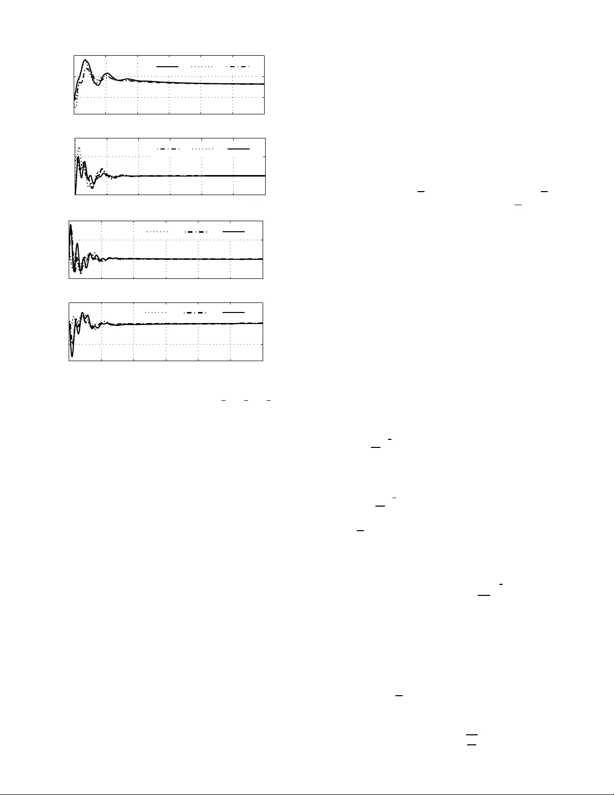
IEEE TRANSACTION ON A UTOMA TIC CONT ROL, MANUSCRIPT FOR R EVIEW 1 Lagrange Stabiliza tion of Pendulum-like Systems: A Pseudo H ∞ Control Approach Hua Ouyang, Member , IEEE, Ian R. Petersen, F ellow , IEEE, and V alery Ugrinovskii, Senior Member , IEEE Abstract —This p aper studi es the Lagrange stabilization of a class of nonlinear systems whose linear part has a singular system matrix and whi ch hav e multiple periodic (i n state) n onlinearities. Both state and output feedback Lagrange stabilization problems are considered. The p aper dev elops a pseudo H ∞ control theory to solve these stabilization problems. In a similar fashion to the Strict Bound ed Real Lemma in classic H ∞ control theory , a Pseudo Strict Bounded Real Lemma is establi shed f or systems with a single u nstable pole. S ufficient conditi ons for the synth esis of state feedback and outp ut feedback controllers ar e given to en sure that the closed-loop system is pseudo strict bound ed real. The pseudo- H ∞ control appro ach i s applied to solve state feedback and output feedback Lagrange stabilization problems fo r n onlinear systems with multiple nonlinearities. An example is giv en to illu strate the p roposed method. Index T erms —Pseudo- H ∞ control, Pseud o S trict Bound ed Real Lemma, Pendulum-like systems, Lagrange stability . I . I N T RO D U C T I O N The class of pen dulum- like systems is a class of nonlin ear systems with periodic (in state) n onlinearities and an infinite number of equilibria [ 1]. Th ey cover an impo rtant class of nonlinear systems arising in electr onics, mech anics and power systems. These systems c an be used to model in terconn ected oscillators, synchro nous electrical machines and electronic phase-locked loop devices [2], [3]. An important control objec- ti ve in r elation to c ontrolling such systems is to ensur e that the closed-loo p system retains the pr operties of a pendu lum-like system and its trajecto ries are bo unded , at least, in the sense o f Lagrang e stability . In combinatio n with oth er analytical to ols, this enables glob al asymp totic pr operties of the system to be established. For example, the monogr aph [1] ma kes extensi ve use of th is ap proach to study g lobal asymptotic behavior of nonlinear systems with p eriodic no nlinearities and an in finite number of e quilibria. The co ncept o f Lagr ange stability can be traced back to H. Poincar ´ e’ s work in the 18 90s [4]. In [5], Lagr ange stability is defined as a pr operty of a state x 0 of a dynamica l system ˙ x = f ( t , x ) given on a metric space S , which req uires that the system trajectory x = x ( f , t , x 0 ) originating at this state x 0 to be contain ed in a b ound ed set. I t is shown in [1] th at if a pend ulum-like system p ossesses both Lagran ge stability and dichotomy , th en it has a so-called gradie nt-like pro perty . The gra dient-like property guarantees that any trajectory of the The authors are with the Univ ersity of New South W ales at the Aus- tralia n Defence Force Academy , Campbell, A CT 2600, Australia e-mails: h.ouyang@ad fa.edu.au, i.r .peter sen@gmail.com, v .ugrino vskii@gmail.c om. Prelimina ry versions of the results of this paper were presente d at the Joint 48th CDC and 28th CCC and the 2010 A CC. This research is supported by the Australia n Research Counci l. pendu lum-like system eventually co n verges to an equilibrium . This is analog ous to the asymptotic stability of a system with a single equ ilibrium. T his o bservation highlig hts the importance of Lag range stability as a to ol to establish the gr adient-like proper ty of pendulum -like systems. It also mo tiv ates th e study of pendulum- like systems within the fram ew ork of Lag range stability which is considered in this pa per . In the au thors’ previous w ork [6], the state feedback con- troller syn thesis p roblem is con sidered for a restricted class of pendu lum-like systems in which the way that the con trolled outputs enter into th e nonlinear ities must h av e a special structure. In con trast to the results in [6], this pap er m ainly focuses on solvin g the outpu t feedback Lagrange stabilization problem for pendu lum-like systems with non linearities which have a gen eral structure. Unlike the spec ial case in [6], in this more general case, a significan tly different metho d utilizin g sign-indefin ite solutions to gam e-type Riccati equations is nec- essary . This ha s led us to develop a p seudo- H ∞ control theory to add ress the Lagr ange stabilization p roblem o f pen dulum- like systems. T his pseud o- H ∞ control theo ry allows a po le of th e closed- loop transfer function to be located in the righ t half of the complex plane and ensu res th at the closed-lo op transfer fun ction satisfies a frequency domain c ondition which is similar to the b ound ed real prop erty [7]. An importan t contribution o f this paper is the pseu do strict boun ded r eal results in Theo rems 3.1 and 3 .2, which are analogous to the standard strict bounded real lemm a [ 8]. Ou r pseu do- H ∞ control theory can be regarded as a theo ry wh ich is an alogou s to the standard H ∞ control theory (see [ 9], [1 0]) but with a non-stand ard closed-lo op stability cond ition. Fu rthermor e, the pap er app lies the propo sed pseudo- H ∞ theory to solve the Lagrang e stabilization p roblem for p endulu m-like systems. The usefulness of the Lagran ge stability property of pendu lum-like systems motivates r esearch o n Lagrang e sta- bilization of pen dulum- like systems; e.g. , see [3], [11]–[1 3]. Howe ver , in these papers it was assumed th at th e no nlinear system co ntains a single nonlinea rity only and has a spec ial matched structure on its n onlinear ity . This special match ed structure en ables th e Lag range stab ilization prob lem to be cast as a standard H ∞ problem . In order to co nsider gen eral sy stem structures which d o no satisfy matc hing con ditions, a different approa ch is required which m otiv ates our pseudo H ∞ control problem . Also , the r esults of [3], [11]–[13] are established using a Lag range stability criterio n giv en in [1] which re quires the linear part of th e system to be minim al. T his means that a post-check is require d on the linear part of the resulting closed- loop system to determin e if it is minimal. In contrast, this paper uses a Lag range stability criterion wh ich does not hav e the IEEE TRANSACTION ON A UTOMA TIC CONT ROL, MANUSCRIPT FOR R EVIEW 2 minimal r ealization requirem ent but uses a strict freq uency- domain condition . This Lagr ange stab ility theory enab les this paper to co nsider a Lag range stabilization pr oblem without the requirem ent of a po st-check on the minim ality of the linear part o f the closed-lo op system. Also, this La grange stability criterion allows u s to solve the Lagrange stabilization problem for nonlinear systems with mu ltiple n onlinearities. I ndeed, a condition of th e stability analysis tech niques used in the paper is th at the closed-loo p system matrix A has a single zero eigenv alue, even th ough multiple nonlin earities are allo wed. The correspond ing condition o n the open-loop system in our control synthesis results is that this system must have a single unobser vable (or unco ntrollable) m ode at the origin. T o illustrate the efficacy of the prop osed m ethod, we give an example. It is con cerned with Lagrang e stabilization o f a network of th ree intercon nected nonlinear pendulu ms. Also, this system has som e of the f eatures of many practical system s such as power systems, large-scale interco nnected n etworks and h ence it sugg ests som e applica tion are as for the theory developed in this p aper . These feature s are an in terconne ction of non linear but not identical elements, and the existence of multip le equilibria points due to the periodicity o f the nonlinear elemen ts. This pap er is organized as fo llows: Section II fo rmulates the Lagra nge stabilization problem for pend ulum-like systems; Section III presents a pseudo H ∞ control th eory , wh ich is motiv ated by the prob lem for mulated in Section 2; Section IV p resents ou r main results on output feedback Lagrang e stabilization of unobservable pendu lum-like systems; Section V pr esents our re sults on the ou tput feedba ck Lagrang e stabilization o f un controllab le pendulum -like systems; Section VI gives results on the state feedb ack Lagrange stabilization of unco ntrollable pen dulum- like systems. Section VII p resents an example to illustrate th e efficacy of the prop osed method and Sectio n VIII con cludes this paper . All of the pr oofs of the theorems in the Section s II-VI are contained in the Appe ndix. Notation: Z denotes the set of integers. R n × m and C n × m denote the space of n × m real matrices and th e space of n × m complex matrices, respectively . Q d enotes th e set of ration al number s and Q m denotes the set of vectors of m rational number s. σ ( A ) d enotes the set of the eigenv alues of a matrix A . σ max [ · ] d enotes the maximum singular value of a matrix. R H ∞ denotes the space o f all proper an d r eal rational stable transfer function matr ices. R + denotes the set o f p ositiv e real nu mbers and R n + = ( R + ) n . ρ ( X ) deno tes the spectral ra dius of the matrix X . diag [ a 1 , · · · , a n ] is a diagon al matrix with a 1 , · · · , a n as its diago nal elements. B ( a , ε ) d enotes a neigh borho od around a ∈ R n , define d as { ˜ a ∈ R n : k ˜ a − a k < ε } . Given a vector τ = [ τ 1 , · · · , τ m ] T ∈ R m + , M τ denotes the d iagonal ma- trix M τ = diag [ τ 1 , · · · , τ m ] . Similarly , M µ = diag [ µ 1 , · · · , µ m ] . Giv en a vector ν ∈ Q m , LCMD ( ν ) den otes the least common multiple ( LCM) of the deno minator s of all th e elements of ν . I I . P RO B L E M F O R M U L AT I O N O F L AG R A N G E S TA B I L I Z A T I O N F O R P E N D U L U M - L I K E S Y S T E M A. P endulum-like Systems W e consider a class of non linear systems defined as follows: ˙ x = Ax + Bw , z = Cx , (1) where x ∈ R n is the state, z ∈ R m is the no nlinearity output vector and w ∈ R m is the non linearity input vector . Also, A ∈ R n × n , B ∈ R n × m , C = [ C T 1 , · · · , C T m ] T ∈ R m × n , C i ∈ R 1 × m , i = 1 , · · · , m . Th e compon ents of the vector w = [ w 1 , · · · , w m ] T are determined from th e correspo nding co mponen ts of the vector z = [ z 1 , · · · , z m ] T via nonlin ear functions w i = φ i ( t , z i ) (2) where φ i : R + × R → R is a contin uous, locally Lipsch itz in the secon d argu ment and per iodic fun ction with period ∆ i > 0; i.e., φ i ( t , z i + ∆ i ) = φ i ( t , z i ) , ∀ t ∈ R + , z i ∈ R . (3) This type of nonlinear ity app ears frequently in th e practical engineer ing systems mentioned in Section I. Phase-locked loops [14] and a pen dulum sy stem with a vib rating p oint of su spension [1] are typical examples of such systems. W e also refer to th e example given in Section VII. The transfer function of the linear pa rt of the system (1) is gi ven by G ( s ) = C ( sI − A ) − 1 B . The non linear fun ctions φ i ( t , z i ) , i = 1 , · · · , m , are assumed to satisfy the sector con ditions, − µ i ≤ φ ( t , z i ) z i ≤ µ i , ∀ t ∈ R + , z i 6 = 0 , (4) where µ i ∈ R + , i = 1 , · · · , m . W e define ∆ ∈ R m × m as ∆ = diag [ ∆ 1 , · · · , ∆ m ] . Given a vector d ∈ R n , let Π ( d ) △ = { k d | k ∈ Z } . Definition 2.1: (P endulu m-like System [1]) T he no nlinear system (1), (2), (3) is pendulu m-like with respect to Π ( d ) if for any solu tion x ( t , t 0 , x 0 ) of (1), (2), (3) with x ( t 0 ) = x 0 , we hav e x ( t , t 0 , x 0 ) + ¯ d = x ( t , t 0 , x 0 + ¯ d ) , for all t ≥ t 0 , and all ¯ d ∈ Π ( d ) . Remark 2.1: This d efinition reflects the fact that the phase portrait of a pend ulum-like system is p eriodic. For example, in th e case of a simple pen dulum, this means th at its position variable can b e rep resented by an an gle between 0 and 2 π . Definition 2.2: (Lagrange Stab ility [1]) The no nlinear sys- tem (1), (2) is said to be Lag range stable if all its solutions are boun ded. B. Lagrange Stabilization P r o blem for P endulum- like Systems The pend ulum-like system to b e stabilized will be a con - trolled version of the nonlinear system (1), (2), (3), (4). That is, the linear p art o f the system is described by the state equ ations ˙ x = Ax + B 2 u + B 1 w , (5a) z = C 1 x + D 12 u , (5b) y = C 2 x + D 21 w , (5c) IEEE TRANSACTION ON A UTOMA TIC CONT ROL, MANUSCRIPT FOR R EVIEW 3 where x ∈ R n , w ∈ R m , z ∈ R m are defined as in ( 1), u ∈ R q is the contro l in put, and y ∈ R p is the measured outp ut. Here, all the matrices are assumed to h av e compatib le dimen sions. Also, the compo nents o f the nonlinearity input w are related to the compo nents of the system outp ut z as in (2) and the no nlinearities φ i have the p roperty (3). Furthermo re, the nonlinear ities are assumed to satisfy the sector conditio n (4). The system b lock diagram is sho wn in Figur e 1. Linear Syst em P S f r a g r e p l a c e m e n t s φ m φ 1 . . . u y w 1 w m z 1 z m K ( s ) Fig. 1. Nonlinear cont rol system with periodic nonlin earitie s. Pr o blem 1: (Outp ut F eedba ck Lagrange Stab ilization) The output f eedback Lag range stabilization p roblem for the n on- linear system (5), (2), (3), ( 4) is to design a linear controller with the tra nsfer fun ction K ( s ) and state-space r ealization: ˙ x c = A c x c + B c y u = C c x c (6) such that the re sulting closed -loop system is p endulum -like and Lagr ange stab le. Pr o blem 2: (Sta te F eedback Lagrange Stabilization) The state f eedback Lag range stabilizatio n p roblem is to design a state feed back contro l law u = K x for th e system ( 5a), (5 b), (2), (3), (4) to e nsure that the r esulting closed- loop sy stem is pendu lum-like and Lagr ange stable. Note that in some cases, it may be possible to design a controller in the form of (6) to asym ptotically stabilize the system (5), (2), (4). Suc h cases are trivial fr om the point of v iew of Lagrang e stabilization. In o rder to rule out these trivial cases and to g uarantee th at the closed-loop system is a pendu lum-like system, we will a ssume that the linear par t o f the systems (5 ) has un contro llable or u nobservable mo des. T o solve the above two problem s, the f ollowing two tech- nical results o f [6] will be used: Lemma 2.1: ( [ 6]) Consider the nonlinear system ( 1), (2), (3). Supp ose d et A = 0 and there exists a vector ¯ d 6 = 0 such that A ¯ d = 0, C i ¯ d 6 = 0 , i = 1 , · · · , m , and ( ∆ ) − 1 C ¯ d ∈ Q m . Also, let ∆ i C i ¯ d = p i q i for all i = 1 , · · · , m , whe re p i , q i 6 = 0 are integers. Let ¯ p be the LCM of p i , i = 1 , · · · , m . Then , the system (1), (2), (3) is pendulu m-like with respect to Π ( d ) where d = ¯ p ¯ d . Lemma 2.2: ( [6]) (Lagrange Stability Criterion) Suppose the sy stem (1), (2), ( 3), (4 ) is a p endulu m-like system. Also, suppo se there exist a constan t λ > 0 a nd a vector τ = [ τ 1 , · · · , τ m ] T ∈ R m + satisfying the fo llowing con ditions: i. A + λ I has n − 1 eigen values with n egati ve real par ts and one with positiv e real part; ii. G T ( − j ω − λ ) M τ G ( j ω − λ ) < M − 1 µ M τ M − 1 µ , for all ω ≥ 0. Then, the no nlinear system (1), (2), ( 3), (4) is Lag range stable. The pro ofs of these two results a ppear in th e journ al version of [6] but are included in the Append ix for completeness. Lemma 2.2 is the key r esult to establish Lagr ange stability of the closed-loop systems un der consideration. It in v olves a frequen cy domain condition, which is similar to the bound ed real property in [7], and a system state matrix A + λ I which has one u nstable eigenv alue. Howe ver , it does not require the minimality of the linear part of the system (1). T o establish these c ondition s in the Lagra nge stabilization prob lems 1 and 2, we develop a pseudo- H ∞ control theory in the next section, which is an alogous to th e standard H ∞ control th eory . I I I . P S E U D O - H ∞ C O N T RO L A. The Pseudo Strict Bounded Real Pr o perty an d the Corr e- sponding Strict Bo unded Real Lemma (SBRL) The bounded rea l p roper ty is an im portant co ncept f re- quently used in the stand ard H ∞ control theo ry . W e begin our development of pseudo H ∞ control with the definition of th e pseudo strict bounded real proper ty , wh ich is an alogous to the standard boun ded real pro perty . Definition 3.1: A ma trix A ∈ R n × n which has n − 1 eigen - values with negati ve real parts and on e eigenv alue with posi- ti ve real part is said to be pseudo-Hurwitz . A symmetric matrix P ∈ R n × n is said to be pseu do-po sitive defin ite if it has n − 1 positive eigen values and one negati ve eigenv alue. Definition 3.2: A lin ear time -in variant (L TI) system (1) is called pseudo strict bounded r eal if the following c ondition s hold: (i) A is p seudo Hurw itz; (ii) max ω ∈ R { σ max [ G ( − j ω ) T G ( j ω )] } < 1 . (7) Theor em 3.1: Consider the L TI system (1). If the Riccati equation A T P + P A + PBB T P + C T C = 0 (8) has a solution P = P T such that P is pseud o-po siti ve d efinite and A + BB T P has no purely imaginar y eigenv alues, then th e system (1) is pseudo strict bou nded real. Theor em 3.2: If the L TI system (1) is p seudo strict bound ed real, then 1) There exists a pseud o-po siti ve definite matrix P = P T such that A T P + P A + PBB T P + C T C < 0 . (9) 2) Furthermo re, if in addition the pair ( A , B ) is stabilizable and the pair ( A , C ) is observable, then the Riccati equation (8) has a stabilizing solu tion P which is pseu do-po siti ve definite. Theorem 3. 1 is an alogou s to the sufficiency part of the strict bound ed real lemma for s ystems with non-minima l rea lizations [8]. Also, Theorem 3.2 is a nalogou s to the necessity part of the strict bounded real lemma fo r systems with non-minimal IEEE TRANSACTION ON A UTOMA TIC CONT ROL, MANUSCRIPT FOR R EVIEW 4 realizations. Theorems 3.1 and 3 .2 are to gether called the pseudo strict b ound ed r eal lemma . The p seudo strict boun ded real lemma gives a relatio nship between state-space cond itions, such as solvability of (8) and pseudo- Hurwitzness of A , an d the freq uency-do main in equal- ity (7). This will allow us to rep lace the frequency domain condition for the closed-loo p system that will app ear in the application o f L emma 2 .2, with a cond ition in the state-space form. This is a key step in the d eriv ation o f a solu tion to Problems 1 an d 2. B. State F eedb ack Pseudo- H ∞ Contr ol The state feedb ack pseu do- H ∞ control problem for the L T I system (5a), (5 b) in volves designing a state f eedback law u = K x which ensur es that the cor respondin g closed- loop system is pseudo strict bounded r eal. In an an alogou s way to H ∞ control theory [9], [ 10], the m ain resu lt of this section presented in the following theorem, gives a suf ficient condition for the existence of a solution to the pr oblem. The fo llowing assumptio n is made o n the system (5a), (5b): Assumption 3. 1: E 1 = D T 12 D 12 > 0. Theor em 3.3: Suppo se Assumption 3.1 holds for the system (5a), (5b) a nd the Riccati equation ( A − B 2 E − 1 1 D T 12 C 1 ) T P + P ( A − B 2 E − 1 1 D T 12 C 1 ) + P ( B 1 B T 1 − B 2 E − 1 1 B T 2 ) P + C T 1 ( I − D 12 E − 1 1 D T 12 ) C 1 = 0 (10) has a solution P = P T such that P is pseud o-po siti ve d efinite and the matr ix A − B 2 E − 1 1 D T 12 C 1 + ( B 1 B T 1 − B 2 E − 1 1 B T 2 ) P (11) has no p urely imaginary eigenv alues. The n, the state feed back control law u = − E − 1 1 ( B T 2 P + D T 12 C 1 ) x (12) solves the state f eedback pseudo- H ∞ control prob lem. T hat is, the resulting closed -loop sy stem is pseud o strict boun ded real. Remark 3.1: In practice, it is usually con venient to u se th e stabilizing solution to the Riccati equation ( 10) in order to construct the r equired state f eedback contr ol law (12). C. Output F eedba ck Pseudo-H ∞ Contr ol Analogou s to th e standard o utput feedb ack H ∞ control problem , th e output f eedback pseudo- H ∞ control prob lem for the system (5) in volves designin g a compensator of the fo rm (6) to make the correspo nding closed-loop system p seudo strict bound ed r eal. The following two theo rems each giv e a sufficient condition for the existence of a solution to the ou tput feedback pseudo- H ∞ control pr oblem fo r a system of the f orm (5). Besides Assumption 3 .1, the following assumptio n is also made on th e system (5): Assumption 3. 2: E 2 = D 21 D T 21 > 0. Theor em 3.4: Suppo se the system (5) satisfies Assum ptions 3.1 and 3.2 and the following condition s are satisfied: (i) The Riccati eq uation ( A − B 2 E − 1 1 D T 12 C 1 ) T X + X ( A − B 2 E − 1 1 D T 12 C 1 ) + X ( B 1 B T 1 − B 2 E − 1 1 B T 2 ) X + C T 1 ( I − D 12 E − 1 1 D T 12 ) C 1 = 0 (13) has a stabilizing solution X = X T which is pseudo- positive definite; (ii) The Riccati eq uation ( A − B 1 D T 21 E − 1 2 C 2 ) Y + Y ( A − B 1 D T 21 E − 1 2 C 2 ) T + Y ( C T 1 C 1 − C T 2 E − 1 2 C 2 ) Y + B 1 ( I − D T 21 E − 1 2 D 21 ) B T 1 = 0 (14) has a stabilizing solutio n Y = Y T which is p ositi ve definite; (iii) The m atrix X Y has a spe ctral rad ius strictly less than one, ρ ( X Y ) < 1. Then, there e xists a dynamic output feed back compe nsator of the form (6) such that the r esulting closed-loop system is pseudo strict boun ded real. Further more, th e matrice s defin ing the requ ired dynam ic feedback controller (6) can b e con- structed as f ollows: A c = A + B 2 C c − B c C 2 + ( B 1 − B c D 21 ) B T 1 X , B c = ( I − Y X ) − 1 ( Y C T 2 + B 1 D T 21 ) E − 1 2 , C c = − E − 1 1 ( B T 2 X + D T 12 C 1 ) . (15) Theor em 3.5: Suppo se the system (5) satisfies Assumptio ns 3.1 and 3.2 and the following co nditions are satisfied: (i) The Riccati equ ation (13) has a p ositiv e d efinite stabilizing solution X = X T ; (ii) the Riccati eq uation (1 4) ha s a pseudo- positive de fi- nite stabilizing solution Y = Y T ; (iii) The m atrix X Y has a spe ctral rad ius strictly less than one, ρ ( X Y ) < 1. Then, ther e exists a dyn amic ou tput feedba ck compen sator of the form (6) such that the r esulting closed-loop system is pseudo strict boun ded real. Furth ermore, the ma trices in the required dy namic feedb ack controller (6) can be co nstructed as follows: A c = A + B c C 2 − B 2 C c + Y C T 1 ( C 1 − D 12 C c ) , B c = − ( Y C T 2 + B T 1 D T 21 ) E − 1 2 , C c = E − 1 1 ( B T 2 X + D T 12 C 1 )( I − Y X ) − 1 . (16 ) Remark 3.2: Accord ing to [1 5], th e stabilizing solutions to the Riccati equations ( 13) and (14) are unique, if th ey exist. I V . O U T P U T F E E D BA C K L AG R A N G E S TA B I L I Z I N G C O N T RO L L E R S Y N T H E S I S F O R U N O B S E RV A B L E S Y S T E M S In this section, the output feedback p seudo H ∞ control theory developed in th e previous section is u sed to solve Problem 1 for non linear systems satisfying the following assumptions, which w ill be used to ensur e th at the clo sed- loop system is pendulu m-like and to rule out trivial cases in which th e n onlinear system can be asymptotically stabilized : Assumption 4.1: There exists a non-zer o vector x such that Ax = 0 and C 2 x = 0. IEEE TRANSACTION ON A UTOMA TIC CONT ROL, MANUSCRIPT FOR R EVIEW 5 Assumption 4. 1 imp lies that ( A , C 2 ) is unobservable and the origin is an unob servable mo de. Using the Kalman decompo - sition in the unob servable form [16], it follows that there exists a no n-singular state-space tran sformation matrix T such that the system matrices o f the sy stem (5) are transformed to the form ˜ A = T − 1 A T =  ˜ A 1 0 ˜ A 2 0  , ˜ B 2 = T − 1 B 2 =  ˜ B 2 a ˜ B 2 b  , ˜ B 1 = T − 1 B 1 =  ˜ B 1 a ˜ B 1 b  , ˜ C 1 = C 1 T =  ˜ C 1 a ˜ C 1 b  , ˜ D 12 = D 12 , ˜ C 2 = C 2 T =  ˜ C 2 a 0  , ˜ D 21 = D 21 , (17) where ˜ A 1 ∈ R ( n − l ) × ( n − l ) , ˜ B 1 a ∈ R ( n − l ) × m , ˜ B 2 a ∈ R ( n − l ) × q , ˜ C 1 a , ˜ C 2 a ∈ R m × ( n − l ) . Also, let e n = [ 0 1 × ( n − 1 ) 1 ] T . W e define two vector s χ = C 1 T e n and ¯ d = [ 0 1 × n e T n T T ] T ∈ R 2 n . Assumption 4. 2: There exists a co nstant τ 0 > 0 such that all the elements of the vector ν = τ 0 ∆ − 1 χ are non -zero rational number s. Remark 4.1: In the case where the coef ficients i n the system (5) are all r ational n umber s, Assumptio n 4.2 amo unts to an assumption that the period s of the nonlin earities are commen- surate. The main result of this s ection in volv es the follo wing Riccati equations depend ent on parame ters λ > 0 and τ i > 0 , i = 1 , · · · , m : ( λ I + A − B 2 ¯ E − 1 1 D T 12 M τ C 1 ) T X + X ( λ I + A − B 2 ¯ E − 1 1 D T 12 M τ C 1 ) + X ( B 1 M µ M − 1 τ M µ B T 1 − B 2 ¯ E − 1 1 B T 2 ) X + C T 1 ( M τ − M τ D 12 ¯ E − 1 1 D T 12 M τ ) C 1 = 0 , (18) ( λ I + A − B 1 M µ M − 1 τ M µ D T 21 ¯ E − 1 2 C 2 ) Y + Y ( λ I + A − B 1 M µ M − 1 τ M µ D T 21 ¯ E − 1 2 C 2 ) T + B 1  M µ M − 1 τ M µ B T 1 − M µ M − 1 τ M µ D T 21 ¯ E − 1 2 D 21 M µ M − 1 τ M µ  B T 1 + Y ( C T 1 M τ C 1 − C T 2 ¯ E − 1 2 C 2 ) Y = 0 , (19) where ¯ E 1 = D T 12 M τ D 12 and ¯ E 2 = D 21 M µ M − 1 τ M µ D T 21 . If these Riccati equatio ns have suitable solutions, we will define th e parameter matrices of the controller (6) as f ollows: A c = A + B c C 2 − B 2 C c + Y C T 1 ( M τ C 1 − M τ D 12 C c ) , B c = − ( Y C T 2 + B 1 M µ M − 1 τ M µ D T 21 ) ¯ E − 1 2 , C c = ¯ E − 1 1 ( B T 2 X + D T 12 M τ C 1 )( I − Y X ) − 1 . (20 ) The fo llowing theo rem, which is the main re sult of this paper, giv es a sufficient condition fo r the existence o f a Lagrang e stabilizing con troller for th e non linear system (5), (2), (3), (4) : Theor em 4.1: Suppo se Assum ptions 3.1, 3.2, 4 .1 and 4.2 hold for the n onlinear system (5), (2), ( 3), (4). Also, sup pose there exist con stants λ > 0 and τ i > 0 , i = 0 , · · · , m such that the fo llowing condition s are satisfied: I. The Riccati equ ation (18) has a stabilizing solution X = X T which is po siti ve definite; II. The Riccati equation (19) has a pseudo-p ositiv e definite stabilizing solu tion Y = Y T ; III. The m atrix X Y has a spe ctral rad ius strictly less than one, ρ ( X Y ) < 1. Then, the resulting clo sed-loop system corr espondin g to the controller (6), (2 0) is a pen dulum- like system with respect to Π ( τ 0 ¯ p ¯ d ) and is Lagrange stable. Here ¯ p = L CMD ( ν ) . V . O U T P U T F E E D BA C K L AG R A N G E S TA B I L I Z I N G C O N T RO L L E R S Y N T H E S I S F O R U N C O N T R O L L A B L E S Y S T E M S In this section, the state f eedback and o utput fee dback pseudo H ∞ control theor ies in Section III are applied to Lagrang e stabilizatio n for nonlinea r systems satisfying the following assum ption which is d ual to Assump tion 4.1: Assumption 5.1: There exists a non-zer o vector x such that x T A = 0 and x T B 2 = 0. In a similar way to Assump tion 4.1, th is assumption is also used to ensure tha t the closed-loop system is pendulum- like and to rule out tri vial cases in which the system can be asymptotically stab ilized. Also, this assumptio n implies that ( A , B 2 ) is not con trollable. Using the Kalm an Deco mposition [16], it follows fr om Assum ption 5.1 that there e xists a no n- singular state-space tra nsformatio n matrix ¯ T su ch that the matrices of the system (5) are tr ansformed to th e form ˜ A = ¯ T − 1 A T =  ˜ A 1 ˜ A 2 0 0  , ˜ B 2 = ¯ T − 1 B 2 =  ˜ B 2 a 0  , ˜ B 1 = ¯ T − 1 B 1 =  ˜ B 1 a ˜ B 1 b  , ˜ D 12 = D 12 , ˜ C 1 = C 1 ¯ T =  ˜ C 1 a ˜ C 1 b  , ˜ C 2 = C 2 ¯ T =  ˜ C 2 a ˜ C 2 b  , ˜ D 21 = D 21 , (21) where ˜ A 1 ∈ R ( n − l ) × ( n − l ) , ˜ A 2 ∈ R ( n − l ) × l , ˜ B 2 a ∈ R ( n − l ) × q , ˜ B 1 a ∈ R ( n − l ) × m , ˜ C 1 a , ˜ C 2 a ∈ R m × ( n − l ) . A. Output F eed back Lagrange Stabilization for Un contr ol- lable Systems The main result of this section in volves the Riccati equations (18) and (19) wh ich are dependent on par ameters λ > 0 and τ i > 0 , i = 1 , · · · , m . Using solutions X an d Y to the equations (18) and (1 9) , we can co nstruct the fo llowing matrice s: A c = A + B 2 C c − B c C 2 +( B 1 M µ M − 1 τ M µ − B c D 21 M µ M − 1 τ M µ ) B T 1 X , B c = ( I − Y X ) − 1 ( Y C T 2 + B 1 M µ M − 1 τ M µ D T 21 ) ¯ E − 1 2 , C c = − ¯ E − 1 1 ( B T 2 X + D T 12 M τ C 1 ) . (22) Also, we defin e two vectors of con stants: ¯ d 0 = −  A c B c ˜ C 2 a ˜ B 2 a C c ˜ A 1  − 1  B c ˜ C 2 b ˜ A 2  , χ =  − D 12 ¯ E − 1 1 ( B T 2 X + D T 12 M τ C 1 ) C 1  ¯ d , ( 23) where ¯ d =  I 0 0 ¯ T   ¯ d 0 1  with ¯ T defined in the Kalm an decomp osition (21). Using this notation, a sufficient condition IEEE TRANSACTION ON A UTOMA TIC CONT ROL, MANUSCRIPT FOR R EVIEW 6 for the solu tion to the outpu t fee dback Lagrange stabilization Problem 1 ca n now b e pr esented: Theor em 5.1: Suppo se Assumptions 3 .1, 3.2 and 5. 1 ho ld for the system (5), (2), (3), ( 4). Also, su ppose there exist constants λ > 0 and τ i , i = 0 , · · · , m such that the f ollowing condition s are satisfied for the nonlin ear system (5), (2), ( 3), (4): I. The Riccati e quation (18) h as a stabilizing pseudo- positive definite solu tion X = X T ; II. The Riccati equ ation (19) has a stabilizing solution Y = Y T which is po siti ve definite; III. The m atrix X Y ha s a spectral rad ius strictly less than one, ρ ( X Y ) < 1; IV . The matr ix  A c B c ˜ C 2 a ˜ B 2 a C c ˜ A 1  is non-sin gular and all the elements of the vector ν = τ 0 ∆ − 1 χ are non- zero rational number s, where A c , B c , C c and χ are defined in ( 22) and (23 ) u sing X , Y in I, I I and III . Then, the clo sed-loop system con sisting of the system (5), (2), (3), ( 4) an d the controller (6), (22) is a pend ulum-like system with r espect to Π λ = { ¯ p τ 0 ¯ d } and is Lag range stable. Here ¯ p = LCMD ( ν ) . B. Satisfaction of th e rationality conditio n. Theorem 5.1 giv es suf ficient condition s for the existence of a solution to the Lagrang e stabilizing contro ller synthesis problem f or a non linear system satisfying Assumption 5 .1. Howe ver , the question arises as to whethe r , given λ > 0 , there will exist positive constan ts τ i , 0 = 1 , · · · , m , such that the stabilizing solu tions to the Riccati equatio ns (18) and (1 9) satisfy the ratio nality cond ition IV of this theor em. First, we demon strate that such τ = [ τ 1 , · · · , τ m ] T , if exists, can b e co nstrained to b e a un it vector . Giv en any γ > 0, let ˆ τ = γ τ , ˜ X = γ X , ˜ Y = γ − 1 Y , M ˆ τ = γ M τ , ˜ E 1 = D T 12 M ˆ τ D 12 and ˜ E 2 = D 21 M − 1 ˆ τ D T 21 . Multiplying the Riccati equation (18) by γ and multip lying (19) by γ − 1 giv es that ( A + λ I − B 2 ˜ E − 1 1 D T 12 M ˆ τ C 1 ) T ˜ X + ˜ X ( A + λ I − B 2 ˜ E − 1 1 D T 12 M ˆ τ C 1 ) + C T 1 ( M ˆ τ − M ˆ τ D 12 ˜ E − 1 1 D T 12 M ˆ τ ) C 1 + ˜ X ( B 1 M µ M − 1 ˆ τ M µ B T 1 − B 2 ˜ E − 1 1 B T 2 ) ˜ X = 0 , (24) ( λ I + A − B 1 M µ M − 1 ˆ τ M µ D T 21 ˜ E − 1 2 C 2 ) ˜ Y + ˜ Y ( λ I + A − B 1 M µ M − 1 ˆ τ M µ D T 21 ˜ E − 1 2 C 2 ) T + ˜ Y ( C T 1 M ˆ τ C 1 − C T 2 ˜ E − 1 2 C 2 ) ˜ Y + B 1 ( M µ M − 1 ˆ τ M µ − M µ M − 1 ˆ τ D T 21 ˜ E − 1 2 D 21 M − 1 ˆ τ M µ ) B T 1 = 0 . (25) It is obvious that (24) has the same form as (18) b ut both X and M τ are scaled by γ . Also, (2 5) has th e same f orm as (1 9) but Y is scaled b y γ − 1 and M τ is scaled by γ . Hence, Conditio ns I-III in th e statement of Theorem 5.1 are n ot affected if we use ˜ X , ˜ Y , M ˆ τ , ˜ E 1 and ˜ E 2 to replace X , Y , M τ , ¯ E 1 and ¯ E 2 respectively . In ad dition, it is straightfor ward to verify that Condition I V o f Theorem 5.1 is not affected by scaling the vector of constants τ . Thu s, without loss of gen erality , we assume that τ is a unit vector th rough out the r emainder of this sectio n, an d if we take τ i > 0 , i = 1 , · · · , m − 1 as independe nt constants combin ed i nto the vector ¯ τ = [ τ 1 , · · · , τ m − 1 ] , then τ m is given b y τ m = s 1 − m − 1 ∑ i = 1 τ 2 i . (26) Define T =  ¯ τ ∈ R m − 1 : Equa tions (18) and (19) have nonsingu lar stabilizing solutions  . Let ˜ τ = [ τ 0 , · · · , τ m − 1 ] T = [ τ 0 , ¯ τ T ] T and d efine a fu nction f ( ˜ τ ) =  f 1 ( ˜ τ ) · · · f m ( ˜ τ )  T = τ 0 ∆ − 1 χ on the set F = { ˜ τ : τ 0 > 0 , ¯ τ ∈ T } . L et J ( τ 0 , τ 1 , · · · , τ m − 1 ) b e the Jacobian matrix of f ( ˜ τ ) , J ( τ 0 , τ 1 , · · · , τ m − 1 ) =     ∂ f 1 ∂ τ 0 ∂ f 1 ∂ τ 1 · · · ∂ f 1 ∂ τ m − 1 . . . . . . . . . . . . ∂ f m ∂ τ 0 ∂ f m ∂ τ 1 · · · ∂ f m ∂ τ m − 1     . (27) Then, we h av e J ( ˜ τ ) = ∆ − 1 ˜ J ( ˜ τ ) and th e elements o f ˜ J ( ˜ τ ) are ˜ J i , 1 = w i , i = 1 , · · · , m ; ˜ J i , j =    τ 0  τ − 2 i w i + τ − 1 i ∂ w i ∂ τ i  : i = j , i = 1 , · · · , m − 1; τ 0 τ − 1 i ∂ w i ∂ τ j : i , j = 1 , · · · , m − 1 , i 6 = j ; ˜ J m , j = τ 0  τ − 3 m τ j w m + τ − 1 m ∂ w m ∂ τ j  , j = 1 , · · · , m . (28) The f ollowing theor em gives a sufficient con dition fo r the existence of the co nstants τ 0 , · · · , τ m satisfying all the condition s of Theorem 5.1: Theor em 5.2: Suppo se Assumptions 3 .1, 3.2 and 5. 1 hold for the system (5), (2), (3), (4). Also, s upp ose there exist a con- stant λ > 0 and a vector of positi ve constants ˜ τ = [ τ 0 , · · · , τ m − 1 ] such that the following condition s are satisfied for the system (5), (2), (3), (4): (I) Conditions I, I I and III of Theore m 5.1 h old; (II) det ˜ J ( ˜ τ ) 6 = 0 wh ere the elements of ˜ J ( ˜ τ ) ar e d efined as (28). Then, given any sufficiently small ε > 0, there exists ˇ τ = [ ˇ τ 0 , ˇ τ 1 , · · · , ˇ τ m − 1 ] ∈ F such that k ˇ τ − ˜ τ k < ε and th e constants τ 0 = ˇ τ 0 , τ i = ˇ τ i , i = 1 , · · · , m − 1 and τ m (defined as in (26)) satisfy all the co nditions of Theor em 5. 1 and henc e th e corr e- sponding closed-lo op system is pe ndulum -like an d Lagrang e stable. V I . S TA T E F E E D B AC K L AG R A N G E S TA B I L I Z A T I O N F O R U N C O N T RO L L A B L E S Y S T E M S In this sectio n, we g iv e a su fficient cond ition fo r the e xis- tence o f a solution to the state f eedback Lagra nge stabilization problem (Pro blem 2) of Section II. Using a solutio n to the Riccati eq uation (18), we de- fine two vectors ¯ d = ¯ T [ ¯ d T 0 1 ] T and χ = [ χ 1 · · · χ m ] T =  I − D 12 ¯ E − 1 1 D T 12 M τ  C 1 − D 12 ¯ E − 1 1 B T 2 X  ¯ d , wher e ¯ T is defined by (21) and ¯ d 0 = − ( ˜ A 1 − ˜ B 2 a ¯ E − 1 1 ˜ D T 12 M τ C 1 a − ˜ B 2 a ¯ E − 1 1 ˜ B T 2 a ¯ X 11 ) − 1 × ( ˜ A 2 − ˜ B 2 a ¯ E − 1 1 ˜ D T 12 M τ C 1 b − ˜ B 2 a ¯ E − 1 1 ˜ B T 2 a ¯ X 12 ) IEEE TRANSACTION ON A UTOMA TIC CONT ROL, MANUSCRIPT FOR R EVIEW 7 with ¯ X 11 ∈ R ( n − 1 ) × ( m − 1 ) , ¯ X 12 ∈ R ( n − 1 ) × 1 defined by ¯ T T X ¯ T =  ¯ X 11 ¯ X 12 ¯ X 12 ¯ X 22  . Theor em 6.1: Consider the nonlinear system (5a), (5b), (2), (3), (4) and suppo se Assumptions 3.1 and 5.1 are satisfied. If ther e exist con stants λ > 0 an d τ i > 0 , i = 0 , · · · , m such that the Riccati equatio n (18) h as a pseu do-po siti ve definite solution X = X T such th at I. The matrix A + λ I − B 2 ¯ E − 1 1 D T 12 M τ C 1 + ( B 1 M µ M − 1 τ M µ B T 1 − B 2 ¯ E − 1 1 B T 2 ) X is Hurw itz; II. All elements of the vector ν = τ 0 ∆ − 1 χ are non-zero rational nu mbers. Then, the closed-lo op system correspo nding to the state feed- back con trol u =  − D 12 ¯ E − 1 1 D T 12 M τ C 1 − D 12 ¯ E − 1 1 B T 2 P  x (29) is a p endulu m-like system with respect to Π  ¯ p τ 0 ¯ d  and is Lagrang e stab le, where ¯ p = LCMD ( ν ) . In a similar way to Theo rem 5.2, a sufficient con dition for the existence of constants τ 0 , · · · , τ m satisfying Condition II o f Theorem 6.1 is now g iv en. The pro of of this result is similar to that o f Theorem 5. 2 and is o mitted. Theor em 6.2: Consider the system (5a), ( 5b), (2), ( 3), (4) and supp ose Assum ptions 3.1, 5 .1 are satisfied. Also, suppose there exists a constant λ > 0 and a vector of positive constants ˜ τ = [ τ 0 , · · · , τ m − 1 ] T satisfying the fo llowing con ditions: I. The Riccati equation ( 18) has a pseud o-positive definite stabilizing solu tion X ; II. ˜ J ( ˜ τ ) 6 = 0 wh ere ˜ J ( ˜ τ ) is defined in (28). Then, giv en any sufficiently small ε > 0, th ere exists a ˇ τ = [ ˇ τ 0 , ˇ τ 1 , · · · , ˇ τ m − 1 ] ∈ F such tha t k ˇ τ − ˜ τ k < ε and the constants τ 0 = ˇ τ 0 , τ i = ˇ τ i , i = 1 , · · · , m − 1 and τ m (defined as in (26)) satisfy all th e conditio ns of Theor em 6.1 and hen ce the correspo nding clo sed-loop system is pend ulum-like and Lagrang e stab le. V I I . I L L U S T R AT I V E E X A M P L E T o illustrate th e theory developed in this pa per, we con sider a system consisting of three conn ected pendulums, as shown in Figure 2, where the pe ndulum s are connected using torsional springs and both pen dulums an d springs are suppo rted by a rigid ring. The pendu lums oscillate in planes perpe ndicular to the ring and the to rsional torque of the spr ings obeys the angular fo rm of the Ho oke’ s law F = − k ∆ θ , where ∆ θ is the angular displacement, F is the spring torque and k is the torque constant. This system can b e co nsidered as a prototy pe of many applicatio ns such as power systems, mechanical s ystems, network systems, etc. The refore, the Lag range stabilization of this system sugg ests many potential applications of the propo sed method. Su ppose that the measuremen ts consist of the angular velocity of a pen dulum and the angula r d ifference between any two neighboring pendulums. As a result, all abso- lute positions of the pe ndulum s a re unobser vable. Also, our A matrix has a single zero eigenv alue wh ich is an uno bservable mode of the system. Hence, Assump tion 4.1 is satisfied. Let x 1 = θ 1 , x 2 = ˙ θ 1 , x 3 = θ 2 , x 4 = ˙ θ 2 , x 5 = θ 3 and x 6 = ˙ θ 3 . Then , the system can be described by the state equations of the fo rm (5) with the following matrices and nonlinearities A =      0 1 0 0 0 0 k 1 + k 3 − α 1 − k 1 0 − k 3 0 0 0 0 1 0 0 − k 1 0 k 1 + k 2 − α 2 k 2 0 0 0 0 0 0 1 − k 3 0 − k 2 0 k 2 + k 3 − α 3      , B 2 =      0 0 0 1 0 0 0 0 0 0 1 0 0 0 0 0 0 1      , B 1 = β      0 0 0 1 0 0 0 0 0 0 1 0 0 0 0 0 0 1      , C 1 = " 1 0 0 0 0 0 0 0 1 0 0 0 0 0 0 0 1 0 # , D 12 = ε 1 I 3 , C 2 = γ " 1 0 − 1 0 0 0 0 0 1 0 − 1 0 0 0 0 0 0 − 1 # , D 21 = ε 2 I 3 , and φ ( z ) = [ sin z 1 sin z 2 sin z 3 ] T . (30) θ1 θ2 θ3 k3 k2 k1 P S f r a g r e p l a c e m e n t s k 1 k 2 k 3 θ 1 θ 2 θ 3 Fig. 2. A s ystem of thre e pendulums connected on a ring by torsional springs. Note that th is system has multiple non linearities and th us the r esults o f [3], [1 1]–[13] can not be ap plied. Also, the nonlinear ities d o not have the special stru cture required in [6] to apply th e result of that paper . The damping coefficients are α 1 = 0 . 1, α 2 = 0 . 0 5, α 3 = 0 . 08. T he tor que con stants are k 1 = 0 . 02, k 2 = 0 . 03 , k 3 = 0 . 05. Also, we specify the constants β = 0 . 2, γ = 0 . 5, ε 1 = ε 2 = 0 . 1. It is easy to verify that the sy stem ( 5), (3 0) satisfies Assump- tion 4 .1. Also, all o f the coefficients of the system (5), (30) are rational. W e choose τ 0 = 2 π to ensur e that Assum ption 4.2 is satisfied ( T will have ratio nal eleme nts in this case). Therefo re, Th eorem 4.1 is app licable to the system. Ch oosing τ 1 = 0 . 4 , τ 2 = 0 . 6 , τ 3 = 0 . 5 and λ = 0 . 5 and solving the Riccati equations (18) and (1 9) g iv es solutions which satisfy all of the co nditions of Theorem 4 .1. Therefore, the solu tion to Prob lem 1 for the system ( 5), (30) can b e con structed using this theore m. T o illustrate the fact that the resulting contro ller is suc h that the closed-loop system is Lagr ange stable, a series of simulations has been carried out with different initial v alues. These simulations have confirme d that th e trajectories of the closed-loo p system are bou nded. This can be seen in Figure IEEE TRANSACTION ON A UTOMA TIC CONT ROL, MANUSCRIPT FOR R EVIEW 8 0 10 20 30 40 50 60 0 5 10 time (sec) 0 10 20 30 40 50 60 −5 0 5 10 time (sec) State Responses x 1 x 3 x 5 x 2 x 4 x 6 0 10 20 30 40 50 60 −1 0 1 2 time (sec) 0 10 20 30 40 50 60 −5 0 5 time (sec) Controller State Responses x c2 x c4 x c6 x c1 x c3 x c5 Fig. 3. System state responses and controlle r state respon ses of the close d- loop system fo r initial va lues [ x 1 ( 0 ) , · · · , x 6 ( 0 )] T = [ − π 4 , 4 , − π 2 , − 3 , π 3 , − 5 ] and x ci = 0 , i = 1 , · · · , 6. 3, which shows the state responses of the system and th e controller state responses f or one set of initial con ditions, when the o utput feedback con troller is applied. In addition, our simulations reveal that the trajectories o f the closed- loop system converge. Using T heorem 1 in [ 17] and th e results in [1], it can b e verified that the c losed-loop system has the proper ty of dich otomy and th e gradien t-like proper ty , which explains the observed conver genc e. V I I I . C O N C L U S I O N S A N D F U T U R E R E S E A R C H This paper has studied the Lagrang e stabilization problem for non linear systems with multiple no nlinearities. In o rder to facilitate the co ntroller synthesis fo r these systems, a pseud o- H ∞ control theor y is developed. Sufficient conditions for the solution to state feedba ck and output feedback pseud o- H ∞ control pro blems are given. Ho wever , correspo nding necessary condition s are y et to be obtained . Th e pseudo- H ∞ control theory is app lied to solve output feedback and state feedback Lagrang e stab ilization prob lems for non linear systems with multiple n onlinearities. The efficacy o f the meth od is illus- trated b y an exam ple in volving coupled n onlinear pen dulums on a r ing. This p aper has co nsidered the c ase wher e the nonlinear system contains decoupled nonlinearities. That is, as illustrated in Figure 1, we consider independ ent scalar nonline arity blocks each su bject to a sector bou nd constraint. One possible area for f uture research is to e xtend the ap proach of this paper to enable th e co nsideration o f nonlinear systems with coupled nonlinear ities. This would inv olve allowing the non linear blocks in Figur e 1 to hav e vector inputs and o utputs and to replace th e sector b ound s by more general local qu adratic constraints. A P P E N D I X A. Pr o of of Lemma 2.1 First note that p i 6 = 0 since ∆ i 6 = 0. From the conditions of the lemma, we h av e E i ¯ d = ∆ i q i p i . From (3 ) and th e fact that q i p i ¯ p is an in teger , it follows that φ i ( t , C i ¯ d + C i x ) = φ i ( t , ∆ i q i p i ¯ p + C i x ) = φ i ( t , C i x ) . As A ¯ d = 0, it follo ws that, A ( x + ¯ d ) + m ∑ i = 1 B i φ i ( t , C i ¯ d + C i x ) = Ax + m ∑ i = 1 φ i ( t , C i x ) , (31) for all x and t . Consider an arbitrary solution x ( t , t 0 , x 0 ) o f the system (1), (2). Let ¯ x ( t ) = x ( t , t 0 , x 0 ) + ¯ d for t ≥ t 0 . Then, ¯ x ( t 0 ) = x 0 + ¯ d . Also, it readily f ollows f rom (31) that ¯ x ( t ) = x ( t , t 0 , x 0 + ¯ d ) . Furthermo re, the local Lipschitz con dition imp lies the uniqu e- ness of this solution . Then, we have ¯ x ( t ) = x ( t , t 0 , x 0 + ¯ d ) = x ( t , t 0 , x 0 ) + ¯ d . Hen ce, the lem ma follows.  B. An Outline of the P r o of of Lemma 2.2: Define G ( x , ξ ) △ = ∑ m i = 1 τ i  − µ − 1 i ξ i − C i x  ∗  µ − 1 i ξ i − C i x  where ξ ∈ C m and x ∈ C n are arbitrary complex vectors. Clearly , th ere exist constants δ > 0 an d 0 < υ < 1 such tha t  ξ ζ  ∗   B T  δ 2 υ  1 2 I   ×  ( − j ω − λ ) I − A T  − 1 C T M τ C ( ( j ω − λ ) I − A ) − 1 ×   B T  δ 2 υ  1 2 I   T  ξ ζ  − ξ ∗ M − 1 µ M τ M − 1 µ ξ − ζ ∗ ζ ≤ − δ 2  ξ ∗ M − 1 µ M τ M − 1 µ ξ + ζ ∗ ζ  , ∀ ω ∈ R , ∀ [ ξ T ζ T ] T ∈ C m + n . (32) Giv en ω ∈ R , we define ¯ σ = (( j ω − λ ) I − A ) − 1 [ B  δ 2 υ  1 2 I ] ¯ ζ and G a  ¯ σ , ¯ ζ  = ¯ σ ∗ C T M τ C ¯ σ − ¯ ζ ∗ M a ¯ ζ , where ¯ ζ =  ξ ζ  and M a =  M − 1 µ M τ M − 1 µ 0 0 I  . Ther efore, it follows from (32) tha t G a  ¯ σ , ¯ ζ  ≤ − δ 2 ¯ ζ ∗ M a ¯ ζ , ∀ ω ∈ R , ¯ ζ ∈ C m + n . (33) Furthermo re, since M a is a positive definite matr ix, the in- equality ( 33) implies that G a  ¯ σ , ¯ ζ  < 0 , for all ¯ ζ ∈ C m + n such that k ¯ ζ k 6 = 0. Also, the pair ( A , [ B q δ 2 υ I n × n ]) is controllable. IEEE TRANSACTION ON A UTOMA TIC CONT ROL, MANUSCRIPT FOR R EVIEW 9 Using Theore m 1.1 1.1 in [1], it follows tha t there exists a Hermitian matrix P = P ∗ satisfying 2 x ∗ P (( A + λ I ) x + B ξ + q δ 2 υ ζ ) + ¯ σ ∗ C T M τ C ¯ σ − ξ ∗ M − 1 µ M τ M − 1 µ ξ − ζ ∗ ζ < 0 , for all x ∈ C n , ¯ ζ = [ ξ T ζ T ] T ∈ C m + n such that k x k + k ξ k + k ζ k 6 = 0. Letting ζ = 0, this implies that th ere exists an n × n matrix P = P T such that 2 x ∗ P [ Ax + B ξ ] < − 2 λ x ∗ Px − G ( x , ξ ) (34) for all x ∈ C n , ξ ∈ C m such th at k x k + k ξ k 6 = 0. Letting ξ = 0 in ( 34), we ob tain that ther e exists a r > 0 such that 2 x T P [ A + λ I ] x < − r x T x < 0. Note that the pair ( A + λ I , rI ) is observable. Since the matrix A + λ I is pseudo-Hu rwitz, then using Theorem 3 in [18] g iv es that P is pseudo-po siti ve definite. In a similar w ay to the proof of Theorem 2.6.1 in [1], we can prove that the set { x ∈ R n : x T Px < 0 } is p ositiv ely inv ariant for the nonlinear system (1), ( 2), (3) a nd f urther p rove that the solution x ( t , t 0 , x 0 ) of the system (1), (2), ( 3) is bo unded .  C. Pr oof of Theo r em 3.1: In orde r to p rove Theorem 3.1, so me p reliminary results a re required . Lemma A.1: Supp ose the pair ( C , A ) has no un observable modes on the j ω axis. If the L yapunov equ ation A T P + P A + C T C = 0 has a pseudo- positiv e definite solutio n P = P T , then the matr ix A is p seudo-Hu rwitz. In order to prove Lemma A.1, we require the following results: Lemma A.2 ( [19 ]): Let ¯ P be a symmetr ic m atrix of the form ¯ P =  0 ¯ P 12 ¯ P T 12 ¯ P 22  , wh ere ¯ P 22 = ¯ P T 22 and ¯ P T 12 are n 2 × n 2 and n 2 × n 1 matrices, respectively . Also, let k △ = rank ( ¯ P T 12 ) . Then In ( ¯ P ) = In ( ¯ P 22 / ker ( ¯ P 12 )) + ( k , k , n 1 − k ) , (35) where ker ( ¯ P 12 ) = { ζ ∈ R m : ¯ P 12 ζ = 0 } and ¯ P 22 / ker ( ¯ P 12 ) rep- resents the r estriction of ¯ P 22 to ker ( ¯ P 12 ) . Lemma A.3 ( [20 ]): If A ∈ R n × n and if λ , µ ∈ σ ( A ) are eigenv alues of A wher e λ 6 = µ , th en any le ft eigenv ector of A correspo nding to µ is orthogo nal to any r ight eigenv ector of A cor respond ing to λ . Pr o of o f Lemma A.1: The Ka lman deco mposition [16] establishes the existence o f a matrix T wh ich transforms the matrix pair ( A , C ) into the form ¯ A = T AT − 1 =  ¯ A 11 ¯ A 12 0 ¯ A 22  , ¯ C = C T − 1 = [ 0 ¯ C 2 ] where the pa ir ( ¯ A 22 , ¯ C 2 ) is observable. The dime nsions of the block s in th e above decomp osition are as follows: ¯ A 11 ∈ R n 1 × n 1 , ¯ A 11 ∈ R n 1 × n 2 , ¯ A 22 ∈ R n 2 × n 2 , and the colu mn dimension of ¯ C 2 is n 2 . Corresp onding ly , let ¯ P = T − T PT − 1 =  ¯ P 11 ¯ P 12 ¯ P T 12 ¯ P 22  . It follows fr om the observ - ability of ( ¯ A 22 , ¯ C 2 ) that there exists a matrix ¯ K such that δ ( ¯ A + ¯ K ¯ C ) = 0 . Using the e quation A T P + P A + C T C = 0, it fo llows that  ¯ A T 11 ¯ P 11 + ¯ P 11 ¯ A 11 ¯ A T 12 ¯ P 11 + ¯ A T 22 ¯ P T 12 + ¯ P T 12 ¯ A T 11 ¯ P 11 ¯ A 12 + ¯ P 12 ¯ A 22 + ¯ A 11 ¯ P 12 ¯ P T 12 ¯ A 12 + ¯ A T 12 ¯ P 12 + ¯ P 22 ¯ A 22 + ¯ A T 22 ¯ P 22 + ¯ C T 2 ¯ C 2  = 0 . (36) Hence, ¯ A T 11 ¯ P 11 + ¯ P 11 ¯ A 11 = 0 . (37) Claim 1: If the pair ( ¯ C , ¯ A ) is such that there exists a matrix ¯ K satisfying δ ( ¯ A + ¯ K ¯ C ) = 0, then Re λ ( ¯ A 11 ) 6 = 0 fo r ∀ λ ∈ σ ( ¯ A 11 ) . T o establish Claim 1, we rewrite ¯ K as ¯ K =  ¯ K 1 ¯ K 2  . Then ¯ A + ¯ K ¯ C =  ¯ A 11 ¯ A 12 + ¯ K 1 ¯ C 2 0 ¯ A 22 + ¯ K 2 ¯ C 2  . If there exists an eigenv alue of ¯ A 11 such that Re λ ( ¯ A 11 ) = 0, then ¯ A + ¯ K ¯ C obvio usly has purely imag inary eigenv alues. This con tradicts the fact that ¯ K is cho sen so that δ ( ¯ A + ¯ K ¯ C ) = 0. There fore, Re λ ( ¯ A 11 ) 6 = 0. This completes the proof of the claim. Combining Claim 1 and (37) gi ves th at ¯ P 11 = 0. Also, the ( 1 , 2 ) blo ck of (36) im plies that ¯ P 12 ¯ A 22 + ¯ A 11 ¯ P 12 = 0 . (38) As ¯ P is nonsingular, this imp lies that ¯ P 12 ¯ P T 12 > 0. Apply- ing Lemma A.2 to ¯ P gives that In ¯ P = In ( ¯ P 22 / ker ¯ P 12 ) + ( rank ¯ P T 12 , rank ¯ P T 12 , n 1 − rank ¯ P T 12 ) . It is known that In ¯ P = ( n − 1 , 1 , 0 ) . This implies th at 1) 0 = δ ( ¯ P ) = δ ( ¯ P 22 / ker ¯ P 12 ) + ( n 1 − r ank ¯ P T 12 ) . For ¯ P T 12 ∈ R n 2 × n 1 , it always holds that ran k ¯ P T 12 ≤ n 1 . Then, δ ( ¯ P 22 / ker ¯ P 12 ) ≤ 0. So, δ ( ¯ P 22 / ker ¯ P 12 ) = 0 holds. This further implies that n 1 = rank ¯ P T 12 . Also, the condition δ ( ¯ P 22 / ker ¯ P 12 ) = 0 implies that th e matrix ¯ P 22 / ker ¯ P 12 is nonsingu lar and has no pure ly im aginary eigenv alues. 2) 1 = ν ( ¯ P ) = ν ( ¯ P 22 / ker ¯ P 12 ) + rank ¯ P T 12 . Hence, ra nk ¯ P T 12 ≤ 1 and ¯ P 12 ¯ P T 12 > 0 imp ly rank ¯ P T 12 = 1 and ν ( ¯ P 22 / ker ¯ P 12 ) = 0. Hence, ¯ P 22 / ker ¯ P 12 △ = S T ¯ P 22 S is symm etric and positive definite, where the colum ns of S form a basis f or ker ¯ P 12 . 3) Finally , the identity π ( ¯ P ) = n − 1 = π ( ¯ P 22 / ker ¯ P 12 ) + rank ¯ P T 12 implies π ( ¯ P 22 / ker ¯ P 12 ) = n − 2 . Therefo re, it follows that n 1 = 1. Hence A 11 is a scalar , ¯ P 12 is a row vector of dimensio n n − 1 , and ¯ P 22 is a ( n − 1 ) × ( n − 1 ) matrix. The dimension o f S T ¯ P 22 S is equal to n − 2 . As ¯ P 12 ∈ R 1 × ( n − 1 ) , ¯ P 12 6 = 0, ( 38) implies that − ¯ A 11 is an eigenv alue of ¯ A 22 and ¯ P 12 is the correspon ding left eigenv ector . Now , let λ be any eigenvalue of ¯ A 22 such that λ 6 = − ¯ A 11 and let q b e a correspon ding rig ht eigenvector; th at is, ¯ A 22 q = λ q . Then Lemma A.3 implies that ¯ P 12 q = 0. Hence, q ∈ Ker ¯ P 12 . Pre- and post-multip lying th e ( 2 , 2 ) block of (36) by q T and q respectively imp lies tha t q T ¯ P 22 ¯ A 22 q + q T ¯ A T 22 ¯ P 22 q + q T ¯ C T 2 ¯ C 2 q = 0. Th erefore , λ q T ¯ P 22 q + ¯ λ q T ¯ P 22 q + k ¯ C 2 q k 2 = 0. Using the fact that α = q T ¯ P 22 q is positive on Ker ¯ P 12 , we have 2 α Re ( λ ) + k ¯ C 2 q k 2 = 0 . Since q 6 = 0 is an eigenvector o f ¯ A 22 , ¯ C 2 q 6 = 0. Th erefore , Re ( λ ) < 0. The above deriv ation shows that all eigenv alues of ¯ A 22 , possibly with the exception of − ¯ A 11 , ha ve negati ve real pa rt. IEEE TRANSACTION ON A UTOMA TIC CONT ROL, MANUSCRIPT FOR R EVIEW 10 Therefo re, if − ¯ A 11 is negati ve, then ¯ A 22 is Hur witz; if − ¯ A 11 is positive, then ¯ A 22 has all the eigen values λ 6 = − ¯ A 11 negativ e except − ¯ A 11 . Now , w e ca n con clude that the spectrum o f ¯ A is σ ( ¯ A ) = {− ¯ A 11 , ¯ A 11 and λ : λ 6 = − ¯ A 11 , Re λ < 0 } . Also, since the pair ( C , A ) has no unob servable m odes on the imaginary ax is, it follows tha t ¯ A 11 6 = 0. Hence, ¯ A is pseu do-Hur witz. This completes the p roof of Lem ma A.1.  Pr o of of Theor em 3 .1 : By assum ption, P is such th at δ ( A + BB T P ) = 0. Letting ¯ C =  B T P C  , ¯ K =  B 0  , it follows that A + ¯ K ¯ C is such that δ ( A + ¯ K ¯ C ) = 0. Ther efore, ( A + ¯ K ¯ C , ¯ C ) has no unobservable mode on the imaginary ax is and hence ( A , ¯ C ) has no uno bservable m ode on the imaginary axis, either . Applying Lemma A.1 to the L yapunov e quation A T P + P A + ¯ C T ¯ C = 0, it follows that A is pseu do-Hur witz. Hence, det ( j ω I − A ) 6 = 0 for a ll ω ∈ R . Now , we show that (7) holds. Since A is pseud o-Hurwitz, then det ( j ω − A ) 6 = 0, ∀ ω ∈ R . He nce, (8) im plies that G ( − j ω ) T G ( j ω ) = I − [ I − B T P ( − j ω I − A ) − 1 B ] T [ I − B T P ( j ω I − A ) − 1 B ] ≤ I (39) for all ω ≥ 0. It follows that max ω ∈ R { σ max [ G ( j ω ) G ( − j ω ) T ] } ≤ 1. Furthermore, note that G ( j ω ) → 0 as ω → ∞ . Now suppose that there exists an ¯ ω ≥ 0 such that max ω { σ max [ G ( − j ω ) T G ( j ω )] } = 1. It fo llows fr om (39) th at there exists a vector z such that [ I − B T P ( j ¯ ω − A ) − 1 B ] z = 0. Hence, det [ I − B T P ( j ¯ ω − A ) − 1 B ] = 0. However , using a standard result on determin ants, it follows th at det [ j ¯ ω I − A − BB T P ] = det [ j ¯ ω I − A ] det [ I − B T P ( j ¯ ω I − A ) − 1 B ] . Thus det [ j ¯ ω I − A − BB T P ] = 0. This con clusion con tradicts th e assumption that δ ( A + BB T P ) = 0. Hence, (7) holds.  D. P r o of of The or em 3.2: Let µ △ =  max ω ∈ R { σ max [( − j ω I − A T ) − 1 C T C ( j ω I − A ) − 1 ] }  1 2 . It follows f rom (7) that there exist an ε ≥ 0 such th at G ( j ω ) G ( j ω ) T ≤ ( 1 − ε ) I . Hence, ε 2 µ 2 C ( j ω I − A ) − 1 ( − j ω I − A T ) − 1 C T ≤ ε 2 I for all ω ≥ 0. Th en, given any ω ≥ 0, C ( j ω I − A ) − 1 ˜ B ˜ B T ( − j ω I − A T ) − 1 C T ≤  1 − ε 2  I , where ˜ B is a non-singu lar m atrix defined b y ˜ B ˜ B T = BB T + ε / 2 µ 2 I . This further implies that ˜ B T ( − j ω I − A T ) − 1 C T C ( j ω I − A ) − 1 ˜ B ≤  1 − ε 2  I (40) for all ω ≥ 0. L et η 2 △ = max ω ∈ R σ max [ ˜ B T ( − j ω I − A T ) − 1 C T C ( j ω I − A ) − 1 ˜ B ] . Hence, ε 2 η 2 ˜ B T ( − j ω I − A T ) − 1 ( j ω I − A ) − 1 ˜ B ≤ ε 2 I , holds for all ω ≥ 0. Fro m (40), it fo llows that gi ven any ω ≥ 0, ˜ G ( − j ω ) T ˜ G ( j ω ) ≤ I (41) where ˜ G ( s ) = ˜ C ( sI − A ) − 1 ˜ B with ˜ C being a non-singular matrix defined so that ˜ C T ˜ C = C T C + ( ε / 2 η 2 ) I . Furtherm ore, (41) implies ˜ G ( j ω ) ˜ G ( − j ω ) T ≤ I . Since A has no eigenv alue o n the j ω -axis an d the p air ( A , ˜ B ) is stabilizable (sin ce it is contr ollable), it fo llows from T heorem 13 .34 in [10] an d (41) that ther e exists a right coprim e factoriza tion ˜ G ( s ) = ˜ N ( s ) ˜ M − 1 ( s ) such that ˜ M ( s ) ∈ R H ∞ is an inn er transfe r fu nction matrix wher e ˜ M ( s ) = ˜ F ( sI − A − ˜ B ˜ F ) − 1 ˜ B + I ∈ R H ∞ , ˜ N ( s ) = ˜ C ( sI − A − ˜ B ˜ F ) − 1 ˜ B ∈ R H ∞ with ˜ F = − ˜ B T ˜ X , a nd the Riccati equ ation A T ˜ X + ˜ X A − ˜ X ˜ B ˜ B T ˜ X = 0 has a solution ˜ X ≥ 0 such that A − ˜ B ˜ B T ˜ X is stable. Since ˜ M ( s ) is an in ner tran sfer fun ction, it follows th at ˜ N ( j ω ) ˜ N T ( − j ω ) = ˜ G ( j ω ) ˜ G T ( − j ω ) ≤ I . App ly- ing the b ound ed real lemma (e.g ., see [7]), the above condition is eq uiv alent to the existence of a stabilizing solu tion to the Riccati equatio n ( A − ˜ B ˜ B T ˜ X ) T ˆ P + ˆ P ( A − ˜ B ˜ B T ˜ X ) + ˆ P ˜ B ˜ B T ˆ P + ˜ C T ˜ C = 0 . ( 42) Let ˜ P = ˆ P − ˜ X . Then substituting th is into (4 2) giv es that ( A T ˜ X + ˜ X A − ˜ X T ˜ B ˜ B T ˜ X ) +( A T ˜ P + ˜ PA + ˜ P ˜ B ˜ B T ˜ P + ˜ C T ˜ C ) = 0 . (43) Therefo re, ( 43) imp lies that A T ˜ P + ˜ PA + ˜ PBB T ˜ P + C T C + ε 2 µ 2 ˜ P 2 + ε 2 η 2 I = 0. This implies that P = ˜ P satisfies (9). This proves the first claim of the t heor em. No w we prove the second claim. From (7), it follows that G ( j ω ) G T ( − j ω ) ≤ I . As the pair ( A , B ) is stabilizable, T heorem 1 3.34 in [10] implies that the re exists a right co prime factorization G ( s ) = N ( s ) M − 1 ( s ) such that M ( s ) ∈ R H ∞ is an in ner transfer function matrix where M ( s ) = F ( sI − A − BF ) − 1 B + I ∈ R H ∞ , N ( s ) = C ( sI − A − BF ) − 1 B ∈ R H ∞ with F = − B T X , a nd the Riccati equ ation A T X + X A − X BB T X = 0 has a solution X ≥ 0 such tha t A − BB T X is stable. Since M ( s ) is an inner tran sfer func tion, it follows that N ( j ω ) N T ( − j ω ) = G ( j ω ) G T ( − j ω ) ≤ I . Ap - plying the boun ded r eal lemma [7], the a bove condition is equiv alent to th e condition that the following Riccati e quation has a stabilizing solution ( A − BB T X ) T ¯ P + ¯ P ( A − BB T X ) + ¯ PBB T ¯ P + C T C = 0 . ( 44) Let P = ¯ P − X . Then sub stituting this in to (45) gives that ( A T X + X A − X T BB T X ) + ( A T P + P A + PBB T P + C T C ) = 0 . (45) Therefo re, the Ri ccati equation (8) has a stabilizing solution. Furthermo re, as the pair ( A , C ) is o bservable, it follows from the Ine rtia th eorem in [21] that th e solution P = P T of the Riccati equation (8) is a pseudo- positive de finite matrix. This completes the p roof.  Pr o of of The or em 3.3: The Riccati equ ation (10) can be written as ( A − B 2 E − 1 1 D T 12 C 1 ) T P + P ( A − B 2 E − 1 1 D T 12 C 1 ) + PB 1 B T 1 P + C T 1 ( I − D 12 E − 1 1 D T 12 ) C 1 − PB 2 E − 1 1 D T 12 ( I − D 12 E − 1 1 D T 12 ) C 1 − PB 2 E − 1 1 B T 2 P − C T 1 ( I − D 12 E − 1 1 D T 12 ) D 12 E − 1 1 B T 2 P = 0 . (46) As the Riccati e quation (10) has a solu tion P = P T which is p seudo-p ositiv e definite, the equation (4 6) also h as th is IEEE TRANSACTION ON A UTOMA TIC CONT ROL, MANUSCRIPT FOR R EVIEW 11 proper ty . Substituting K = − E − 1 1  D T 12 C 1 + B T 2 P  into (46) implies that ( A + B 2 K ) T P + P ( A + B 2 K ) + PB 1 B T 1 P +( C 1 + D 12 K ) T ( C 1 + D 12 K ) = 0 (47) has a solution P = P T which is pseudo- positive definite. Also, the fact that the m atrix (1 1) h as n o purely im aginary eigenv alues implies that A + B 2 K + B 1 B T 1 P has no pur ely imaginary e igenv alues. Th erefore , it follows from Th eorem 3.1 that the resulting closed-lo op system ˙ x =  A − B 2 E − 1 1 D T 12 C 1 − B 2 E − 1 1 B T 2 P  x + B 1 w , z = C 1 − D 12 E − 1 1  D T 12 C 1 + B T 2 P  x is pseud o strict bou nded real. Th is com pletes the proof o f Theorem 3.3.  E. Pr o of of The or em 3.4 In ord er to p rove Theorem 3. 4, the following lemma is introdu ced. Lemma A.4: Supp ose the condition s of Theorem 3.4 hold. Then, the matrix Z △ = ( I − Y X ) − 1 Y = Y ( I − X Y ) − 1 > 0 is a stabilizing solution to the Riccati equation A ∗ Z + Z A T ∗ − Z M ∗ Z + N ∗ = 0 (48 ) where A ∗ = A − B 1 D T 21 E − 1 2 C 2 + B 1 ( I − D T 21 E − 1 2 D 21 ) B T 1 X , N ∗ = B 1 ( I − D T 21 E − 1 2 D 21 B − 1 1 ) , M ∗ = ( C 2 + D 21 B T 1 X ) T E − 1 2 ( C 2 + D 21 B T 1 X ) − ( B T 2 X + D T 12 C 1 ) T E − 1 1 ( B T 2 X + D T 12 C 1 ) . The p roof of this lem ma is similar to th at of Lemma 3 .2 in [8] and is om itted. Pr o of o f Theorem 3.4 : W e will pr ove that the compen sator of the form (6), ( 15) makes the closed-loop system p seudo strict b ounde d real. I n order to establish this fact, note that Lemma A.4 imp lies that matrix Z = ( I − Y X ) − 1 Y > 0 is a stabilizing solutio n to the Riccati equ ation (48). Sub stituting ( I − Y X ) − 1 Y = Z and ( I − Y X ) − 1 = ( I + Z X ) into ( 15), it follows that the com pensator input ma trix B c can b e written as B c = B 1 D T 21 E − 1 2 + Z ( C T 2 + X B 1 D T 21 ) E − 1 2 . (49 ) W e now form the closed-loop s ystem associated with system (5) a nd compensator (6) . This system is described by the state equation ˙ η = ¯ A η + ¯ Bw , z = ¯ C η , (50) where η △ =  x x − x c  , ¯ A △ =  A + B 2 C c − B 2 C c A − A c + B 2 C c − B c C 2 A c − B 2 C c  , ¯ B △ =  B 1 B 1 − B c D 21  and ¯ C △ =  C 1 + D 12 C c − D 12 C c  . In orde r to verify that this system is p seudo strict boun ded real, we first r ecall that Z > 0 is a stabilizing solu tion to the Riccati equation (48). This implies that Z > 0 will also be a stabilizing solution to the Riccati equation A 0 Z + Z A T 0 + ZC T 0 C 0 Z + B 0 B T 0 = 0 (51 ) where A 0 △ = A − B 1 D T 21 E − 1 2 C 2 + B 1 ( I − D T 21 E − 1 2 D 21 ) B T 1 X − Z ( C 2 + D 21 B T 1 X ) T E − 1 2 ( C 2 + D 21 B T 1 X ) , B 0 △ = B 1 ( I − D T 21 E − 1 2 D 21 ) − Z ( C 2 + D 21 B T 1 X ) T E − 1 2 D 21 , C 0 △ = E 1 2 1 ( B T 2 X + D T 12 C 1 ) . Let W = Z − 1 > 0, then th e Riccati e quation (51) leads to A T 0 W + W A 0 + W B 0 B T 0 W + C T 0 C 0 = 0 . (52) Now , we p rove that W = W T is an anti-stabilizin g solution of (52). Using the Riccati equation (52), it follows that − ( A 0 + ZC T 0 C 0 ) = Z ( A T 0 + Z − 1 B 0 B T 0 ) Z − 1 . He nce the matrix − ( A T 0 + ZC T 0 C 0 ) is similar to th e matr ix ( A 0 + B 0 B T 0 W ) T . Since Z is a stabilizing solution to (5 1), th e matrix A T 0 + ZC T 0 C 0 must be Hurwitz and hence the matrix A 0 + B 0 B T 0 W must be anti- Hurwitz; i.e., W is an an ti-stabilizing solutio n to (52). Now , we define Σ △ =  X 0 0 W  . As X is pseudo- positiv e definite and W > 0, it follows that Σ is also p seudo-p ositiv e definite. Using equ ations (13), (15), (49), (52), it is straig ht- forward to verify tha t Σ satisfies the Riccati equation ¯ A T Σ + Σ ¯ A + Σ ¯ B ¯ B T Σ + ¯ C T ¯ C = 0. Furthermo re, it is straig htforward to verify tha t ¯ A + ¯ B ¯ B T Σ =  ˇ A 11 ˇ A 12 0 A 0 + B 0 B T 0 W  where ˇ A 11 = A − B 2 E − 1 1 D T 12 C 1 − ( B 2 E − 1 1 B T 2 − B 1 B T 1 ) X , ˇ A 12 = B 2 E − 1 1 B T 2 + B 2 E − 1 1 D T 12 C 1 + B 1 ( I − D T 21 E − 1 2 D 21 ) B T 1 W − B 1 D T 21 E − 1 2 ( C 2 + D T 21 ) ZW . Using the fact that X is a stabilizing solution to (13) an d W is an an ti-stabilizing solution to ( 52), it follows that ¯ A + ¯ B ¯ B T Σ h as no pu rely imag inary eig en values. W e have noted p reviously that the matrix Σ is pseud o-positive definite. Therefore, using Theor em 3. 1, we conc lude th at th e system (50) is pseu do strict bou nded real. Using the fact that η =  I 0 I − I   x x c  , it follows that the closed-lo op system  ˙ x ˙ x c  =  A B 2 C c B c C 2 A c   x x c  +  B 1 B c D 21  w ; z =  C 1 D 12 C c   x x c  is also p seudo strict bo unded real. This completes the p roof of Theo rem 3.4.  F . Pr o of of Th eor em 3.5: Consider the system described by the state eq uations ˙ ˜ x = ˜ A ˜ x + ˜ B 2 ˜ u + ˜ B 1 ˜ w , ˜ z = ˜ C 1 ˜ x + ˜ D 12 ˜ u , ˜ y = ˜ C 2 ˜ x + ˜ D 21 ˜ w , (53) where ˜ A = A T , ˜ B 1 = C T 1 , ˜ B 2 = C T 2 , ˜ C 1 = B T 1 , ˜ D 12 = D T 21 , ˜ C 2 = B T 2 , ˜ D 21 = D T 12 , (54) Let ˜ E 1 = ˜ D T 12 ˜ D 12 = E 2 , ˜ E 2 = ˜ D T 21 ˜ D 21 = E 1 , ˜ X = Y , ˜ Y = X . (55) Substituting th e matric es in (54) and ( 55) into Cond itions (i), (ii), ( iii) of the th eorem gi ves th at th e system ( 53) satisfies the following conditions of Theo rem 3.4: IEEE TRANSACTION ON A UTOMA TIC CONT ROL, MANUSCRIPT FOR R EVIEW 12 (i’) The Riccati, as shown below , has a p seudo-p ositiv e definite stabilizing solu tion ( ˜ A − ˜ B 2 ˜ E − 1 1 ˜ D T 12 ˜ C 1 ) T ˜ X + ˜ X ( ˜ A − ˜ B 2 ˜ E − 1 1 ˜ D T 12 ˜ C 1 ) + ˜ X ( ˜ B 1 ˜ B T 1 − ˜ B 2 ˜ E − 1 1 ˜ B T 2 ) ˜ X + ˜ C T 1 ( I − ˜ D 12 ˜ E − 1 1 ˜ D T 12 ) ˜ C 1 = 0 . (56) (ii’) The following Riccati equation has a positive definite stabilizing solution ( ˜ A − ˜ B 1 ˜ D T 21 ˜ E − 1 2 ˜ C 2 ) ˜ Y + ˜ Y ( ˜ A − ˜ B 1 ˜ D T 21 ˜ E − 1 2 ˜ C 2 ) T + ˜ Y ( ˜ C T 1 ˜ C 1 − ˜ C T 2 ˜ E − 1 2 ˜ C 2 ) ˜ Y + ˜ B 1 ( I − ˜ D T 21 ˜ E − 1 2 ˜ D 21 ) ˜ B T 1 = 0 . (57) (iii’) The m atrix ˜ X ˜ Y h as a spe ctral rad ius strictly less than one, ρ ( ˜ X ˜ Y ) < 1. Using Theorem 3 .4, it follows that th ere exists a dyn amic output feedback com pensator of the for m (6) such that the closed-loo p system con sisting of the system (53) a nd this compen sator is pseu do strict bound ed real. The parameters of this co mpensator are as follo ws: ˜ A c = ˜ A + ˜ B 2 ˜ C c − ˜ B c ˜ C 2 + ( ˜ B 1 − ˜ B c ˜ D 21 ) ˜ B T 1 ˜ X , ˜ B c = ( I − ˜ Y ˜ X ) − 1 ( ˜ Y ˜ C T 2 + ˜ B 1 ˜ D T 21 ) ˜ E − 1 2 , ˜ C c = − ˜ E − 1 1 ( ˜ B T 2 ˜ X + ˜ D T 12 ˜ C 1 ) . (58) Substituting th e matrix in (54) and (55) into (58), the transfer function of this closed-loo p system b ecomes ˜ G ( s ) =  B T 1 D T 21 B T c   sI −  A T C T 2 B T c C T c B T 2 A T c  − 1  C T 1 C T c D T 12  . Consider the system (5) with co mpensator ( 6) wh ose pa- rameters ar e determ ined b y (1 6). It is readily seen that the transfer functio n o f this clo sed-loop system ˇ G ( s ) satisfies ˇ G ( s ) = ˜ G T ( s ) . Therefor e, fro m the fact that the system (53), (54), (55), (58) is pseudo strict b ound ed real, it f ollows that max ω σ max [ ˇ G T ( − j ω ) ˇ G ( j ω )] < 1. Also,  ˜ A ˜ B 2 ˜ C c ˜ B c ˜ C 2 ˜ A c  T =  A B 2 C c B c C 2 A c  and is p seudo-Hu rwitz. Hence, the clo sed- loop system (5 ), (6), ( 16) is pseud o strict bo unded real.  G. P r o of of The or em 4.1: W e first prove tha t the closed- loop system  ˙ x c ˙ x  =  A c B c C 2 B 2 C c A   x c x  +  B c D 21 B 1  w , z =  D 12 C c C 1   x c x  , (59) obtained by sub stituting the contr oller (6), (20) in to the system (5), is pendulum -like. Let ¯ d = [ 0 1 × n e T n T T ] T . Note the identity  I 0 0 T  − 1  A c B c C 2 B 2 C c A  ¯ d =   A c B c C 2 a 0 B 2 a C c ˜ A 1 0 B 2 b C c ˜ A 2 0    0 ( 2 n − 1 ) × 1 1  = 0 . Since  I 0 0 T  is non -singular, it follows that  A c B c C 2 B 2 C c A  ¯ d = 0. Using this fact and Assumption 4.1, it f ollows from Lemma 2.1 that the resulting closed-loo p system (59) is pen dulum-like system with r espect to the set Π ( τ 0 ¯ p ¯ d ) . From the o utput feedback p seudo H ∞ control theory in Section III, Conditions I, II, III of the theorem imply that the matr ix  λ I + A B 2 C c B c C 2 λ I + A c  is p seudo-Hu rwitz and the fr equency-d omain con dition max ω σ max [ ¯ G T ( − j ω ) ¯ G ( j ω )] < 1 holds, where ¯ G ( · ) is defined as ¯ G ( s ) △ = M 1 2 τ G c ( s ) M − 1 2 τ and here G c ( s ) △ =  C 1 D 12 C c   s −  λ I + A B 2 C c B c C 2 λ I + A c  − 1  B 1 B c D 21  . Then, it fo llows that G T c ( − j ω ) M τ G c ( j ω ) < M − 1 µ M τ M − 1 µ for all ω ∈ R . Now , all the con ditions o f Lemma 2.2 are satisfied and hence the closed-lo op non linear system ( 59), (2), (3), (4) is Lagran ge stable.  H. P r o of of The or em 5.1: W e first prove that the closed- loop system (59), o btained by ap plying the compensator (6), (22) to the system (5), is a pendu lum-like system. Since  I 0 0 ¯ T  − 1  A c B c C 2 B 2 C c A  ¯ d =    A c B c ˜ C 2 a ˜ B 2 a ˜ A 1   B c ˜ C 2 b ˜ A 2  0 1 × ( n − 1 ) 0    ¯ d 0 1  = 0 and  I 0 0 ¯ T  is a no n-singu lar matrix, it follo ws that  A c B c C 2 B 2 C c A  ¯ d = 0. Using this fact and Condition IV of the theo rem, it follows fro m Lemma 2 .1 that the augmen ted closed-loo p system (59), (2 ), (3), (4) is a pendu lum-like system with respect to Π ( ¯ p τ 0 ¯ d ) . Using the outp ut feed back p seudo H ∞ control theory given in Sectio n II I, it follows from Conditions I, II an d III of the theorem that the closed-lo op system (59) is pseudo strict bound ed real. In a similar w ay to the proo f of Theorem 4.1, we have G T c ( − j ω − λ ) M τ G c ( j ω − λ ) < M − 1 µ M τ M − 1 µ . Now , using Lemma 2. 2, it f ollows that the closed-loop system (59), (2 ), (3), (4) is Lagrange stable.  I. Pr o of of Th eor em 5.2 The stabilizing solutions to the Riccati equatio ns (18) and (19) ar e fu nctions of the vector o f co nstants ¯ τ . T o high light this, we use the notation X ( ¯ τ ) and Y ( ¯ τ ) . In the proof of Theorem 5.2, we use the following lemma: Lemma A.5: The nonsing ular stabilizing solutions X ( ¯ τ ) an d Y ( ¯ τ ) to Riccati equation s (18) a nd (19) are r eal analytic function s on the set T . IEEE TRANSACTION ON A UTOMA TIC CONT ROL, MANUSCRIPT FOR R EVIEW 13 Pr o of: As X ( ¯ τ ) is nonsing ular , we can rewrite the Riccati equation (18) as ( λ I + A − B 2 ¯ E − 1 1 D T 12 M τ C 1 ) + B 1 M µ M − 1 τ M µ B T 1 X ( ¯ τ ) − B 2 ¯ E − 1 1 B T 2 X ( ¯ τ ) = − X − 1 ( ¯ τ )  ( λ I + A − B 2 ¯ E − 1 1 D T 12 M τ C 1 ) T + C T 1 ( M τ − M τ D 12 ¯ E − 1 1 D T 12 M τ ) C 1 X − 1 ( ¯ τ )  × X ( ¯ τ ) . (60) As X ( ¯ τ ) is a pseudo -positive definite stabilizing solution to the Riccati eq uation (18), it fo llows that the matrix − ( λ I + A − B 2 ¯ E − 1 1 D T 12 M τ C 1 ) T − C T 1 ( M τ − M τ D 12 ¯ E − 1 1 D T 12 M τ ) C 1 X − 1 ( ¯ τ ) is Hurwitz a nd hence the pair ( − ( λ I + A − B 2 ¯ E − 1 1 D T 12 M τ C 1 ) T , − C T 1 ( M τ − M τ D 12 ¯ E − 1 1 D T 12 M τ ) C 1 ) is stabilizable. The Riccati eq uation (18) ca n be wr itten as X − 1 ( ¯ τ )( λ I + A − B 2 ¯ E − 1 1 D T 12 M τ C 1 ) T +( λ I + A − B 2 ¯ E − 1 1 D T 12 M τ C 1 ) X − 1 ( ¯ τ ) +( B 1 M µ M − 1 τ M µ B T 1 − B 2 ¯ E − 1 1 B T 2 ) + X − 1 ( ¯ τ ) C T 1 ( M τ − M τ D 12 ¯ E − 1 1 D T 12 M τ ) C 1 X − 1 ( ¯ τ ) = 0 . (61) Substituting the matrices − ( λ I + A − B 2 ¯ E − 1 1 D T 12 M τ C 1 ) T , C T 1 ( M τ − M τ D 12 ¯ E − 1 1 D T 12 M τ ) C 1 and − B 1 M µ M − 1 τ M µ B T 1 + B 2 ¯ E − 1 1 B T 2 into A , R an d Q o f Theorem 2 in [22], respectively , it fo llows th at X − 1 ( ¯ τ ) is the max imal solution for all solutions of the Riccati equation (61). Since C T 1 ( M τ − M τ D 12 ¯ E − 1 1 D T 12 M τ ) C 1 ≥ 0 and − B 1 M µ M − 1 τ M µ B T 1 + B 2 ¯ E − 1 1 B T 2 is Hermitian, Theorem 4.1 in [23] is applicable. Usin g Theor em 4 .1 in [2 3] by sub stituting − ( λ I + A − B 2 ¯ E − 1 1 D T 12 M τ C 1 ) T , C T 1 ( M τ − M τ D 12 ¯ E − 1 1 D T 12 M τ ) C 1 and − B 1 M µ M − 1 τ M µ B T 1 + B 2 ¯ E − 1 1 B T 2 into A , R an d Q , respectively , gives X − 1 ( ¯ τ ) is a rea l analytic fu nction of ¯ τ ∈ T . This furth er implies that X ( ¯ τ ) is a r eal analytic fun ction of ¯ τ ∈ T . Similarly , we can verif y that Y ( ¯ τ ) is also a real analytic fun ction of ¯ τ ∈ T .  Pr o of o f Theorem 5.2: Let ε > 0 b e ch osen to b e sufficiently small so that th e set B ( ˜ τ , ε ) =  ¯ τ ∈ R m + : k ¯ τ − ˜ τ k < ε  ⊂ { ˜ τ ∈ F : Condition I, II and II I of Theo rem 5.1 ho lds } . The existence of such an ε > 0 f ollows fro m Lemma A.5. Since X ( ¯ τ ) and Y ( ¯ τ ) are ana lytic function on the set T , it straightfor ward to verify th at f ( ˜ τ ) is an analytic function o n the set F . Since ∆ − 1 is a d iagonal po siti ve definite matrix, it fo llows that Condition II of the theorem imp lies that det J ( ˜ τ ) 6 = 0 . Let c = f ( ˜ τ ) . It follows from the In verse Function Theorem ( e.g., see Theorem 7 .8 in [24]) that th ere is an o pen ball B ( c , ι ) and a unique con tinuously differentiable functio n g from B ( c , ι ) into B ( ˜ τ , ε ) such that ˜ τ = g ( c ) and f ( g ( ¯ c )) = ¯ c for all ¯ c ∈ B ( c , ι ) . Since the set of rationa l vectors Q m is d ense in R m , we c an choose ˇ c ∈ B ( c , ι ) such that all th e elements o f ˇ c are rational and non-ze ro. Also, it fo llows fro m th e above discussion tha t there exists a poin t ˇ τ ∈ B ( ˜ τ , ε ) such that f ( ˇ τ ) = ˇ c where ˇ τ = g ( ˇ c ) . Theref ore, Con dition IV o f Theorem 5.1 is satisfied. It fo llows f rom the definition of B ( ˜ τ , ε ) th at ˇ τ satisfies Conditions I , II and III of Theorem 5.1. Hence, Th eorem 5.1 implies that the correspo nding clo sed-loop system is pendu lum-like and Lagr ange stable.  J. Pr o of of Th eor em 6.1: Substituting the con troller law (29) into the system (5 a), (5b) gives the closed-loop system ˙ x =  A − B 2 ¯ E − 1 1 D T 12 M τ C 1 − B 2 ¯ E − 1 1 B T 2 X  x + B 1 ξ , z =  I − D 12 ¯ E − 1 1 D T 12 M τ  C 1 − D 12 ¯ E − 1 1 B T 2 X  x . (62 ) Since T − 1 ( A − B 2 ¯ E − 1 1 D T 12 M τ C 1 − B 2 ¯ E − 1 1 B T 2 X ) ¯ d = ( ˜ A − ˜ B 2 ¯ E − 1 1 D T 12 M τ ˜ C 1 − ˜ B 2 ¯ E − 1 1 ˜ B T 2 ¯ X ) ¯ d = 0, it follows that ( A − B 2 ¯ E − 1 1 D T 12 M τ C 1 − B 2 ¯ E − 1 1 B T 2 X ) ¯ d = 0. Using this fact and condition II, it follows fro m Lem ma 2. 1 that the closed-lo op system ( 62) is a pendu lum-like sy stem with respe ct to Π ( ¯ p τ 0 ¯ d ) . Using the fact that the Riccati equation (18) has a pseudo- positive definite solution a nd Cond ition I ho lds, Th eorem 3.3 imp lies th at the clo sed-loop system (62) is pseudo strict bound ed rea l. Th en, using Lemma 2 .2, it follows that the closed-loo p system (62), (5 b), (2), ( 3), ( 4) is La grange stable.  R E F E R E N C E S [1] G. Leonov , D. V . Ponomare nko, an d V . Smirno v a, F r equency -domain methods for nonlinear analysis . W orld Scientific, 1996. [2] V . V . Shakhgil’ dyan and L. N. Belyustina , P hase lock ed system (in Russian) . Mosco w: Radi o i Svyaz’, 1982. [3] J. W ang, Z. Dua n, and L. Huang, “Co ntrol of a cla ss of pendulum- lik e systems with Lagrange stability , ” Automa tica , vol. 42, no. 1, pp. 145–150, 2006. [4] H. Poincar ´ e, Les m ´ ethodes nouvelle s de la m ´ ecanique c´ eleste . New Y ork: Do ver Publicati ons Inc., 1957, vol. 3. [5] V . Nemytskii and V . Stepanov , Qualitati ve theory of dif fer ential equa- tions . Ne w Jerse y: Prince ton Uni v . Press, 1960. [6] H. Ouyang, I. R. Petersen, and V . Ugrinovskii, “Control of a pendulum- lik e system with multiple nonline arities, ” in Procee dings of the 17th IF AC W orld Congr ess , Seoul, South Korea, 2008 (Its journal version is under rev ie w). [7] B. D. O. Anderson and S. V ongpani tlerd, Network Analysis and Synthe- sis . Engle wood Cli ffs, NJ: Prenti ce Hall , 1973. [8] I. R. Peterse n, B. D. O. Anderson, and E . A. Jonckheere, “ A first prin- ciple s solution to the non-singula r H ∞ control problem, ” Internati onal J ournal of Robust and Nonlinear Contr ol , vol. 1, no. 3, pp. 171–185, 1991. [9] I. Petersen, V . Ugrinovski, and A. Savkin, Robust Contr ol Design using H ∞ Methods . Springer -V erlag London, 2000. [10] K. Zhou, J. Doyle, and K. Glov er , Robust and Optimal Contr ol . Upper Saddle Riv er , NJ: Prentice-Ha ll, 1996. [11] Y . Y ang and L. Huang, “ H ∞ control ler synthesis for pendulum-lik e systems, ” Syste ms and Contr ol Letters , vol . 50, pp. 263–276, 2003. [12] X. Li and J . Zhong, “Robust lagrange stabilizati on of uncertain pendulum-l ike systems based on nonloca l reduct ion method (in Chi- nese), ” Acta Scientiarum Natural ium U niver sitatis P ekinensis , vol. 41, no. 3, pp. 358–365, 2005. [13] Q. Gao, “Lagrange stabili sation for uncertain phase-control led systems, ” Internati onal Journa l of Contr ol , vol. 82, no. 5, pp. 970–979, 2009. [14] G. Leono v , “Phase synchronizati on: Theory and appli cations, ” Automa- tion and Remote Contr ol , vol. 67, no. 10, pp. 1573–1609, 2006. [15] T . Basar and P . Bernha rd, H ∞ -Optimal Contr ol and Related Minimax Design Pr oblems: A Dynamic Game Appr oac h, Second Edition . Boston: Birkh ¨ auser , 1995. [16] P . Antsaklis an d A. Michel, Linear systems , 2nd ed. Boston, USA: Birkhause r , 2006. [17] Z . Duan, J. W ang, and L. Huang, “Criteri a for dichotomy and gradient- lik e behavio r of a class of nonlinear systems with m ultipl e equilibria, ” Automat ica , vol . 43, no. 9, pp. 1583–1589, 2007. [18] C.-T . Chen, “ A generaliz ation of the inertia theorem, ” SIAM Journal on Applied Mathematic s , vol. 25, no. 2, pp. 158–161 , 1973. IEEE TRANSACTION ON A UTOMA TIC CONT ROL, MANUSCRIPT FOR R EVIEW 14 [19] H. Jongen, T . M ¨ obert, J. R ¨ uckmann, and K. T ammer, “On inertia and Schur comple ment in opti mization, ” Linear Algebr a and its Appli cations , vol. 95, pp. 97–109, Oct. 1987. [20] R. A. Horn and C. R. Johnson, Matrix Analysis . Cambridge , UK: Cambridge Univ ersity Press, 1985. [21] C.-T . Chen, “Inerti a theorem for general matrix equations, ” Journal of Mathemat ical A nalysis and Applications , vol. 49, no. 1, pp. 207–210, Jan. 1975. [22] H. W imm er , “Monoto nicity of maximal solutions of algebr aic Ri ccati equati ons, ” Systems & Contr ol Lette rs , vol. 5, 1985. [23] A. Ran and L. Rodman, “On parameter dependenc e of solutions of algebra ic Riccati equations, ” Mathematics of Contr ol, Signals, and Systems (MCSS) , vo l. 1, no. 3, pp. 269–284, 1988. [24] N. B. Haaser and J. A. S ulli v an, Real A nalysis . V an Nostrand Reinhold Compan y , 1971. Hua Ouyang Hua Ouyang recei ved his B. Eng in Engineering Mec hanics from Hunan Uni ve rsity , China and M.S . degree in Dynamics and Control from Pekin g Univ ersity , China in 2000 and 2003, respect iv ely . He obta ined his first Ph.D. de gree in Industria l Electronics from the Uni ve rsity of Glam- organ , UK and his second Ph.D. degree in Control Theory and Applicat ions from the Univ ersity of Ne w South W ales at the Australian Defence Forc e Academy in 2007 and 2011, respecti vel y . Now , he is a research fello w in the School of Chemica l Engineeri ng, Univ ersity of New South W ales, Australia. His research interests include robust control and filtering, network ed control systems and nonlinear systems (feedback line arizati on, pendulum-li ke systems and fl o w contr ol). Ian Peter sen was born in V ictoria , Australia. He recei ved a Ph.D in Electrical Engine ering in 1984 from the Univ ersity of Rochester . From 1983 to 1985 he was a Postdoctoral Fello w at the Australian Nationa l Univ ersity . In 1985 he joined the Uni ve rsity of Ne w S outh W ales at the Australian Defence Force Academy where he is currentl y Scientia Professor and an Australia n Rese arch Council Federation Fel- lo w in the School of Information T echnolog y and Electric al Engineer ing. He has served as an Asso- ciate E ditor for the IEEE Transact ions on Automatic Control, Systems and Control L etters, Automatica, and SIAM Journal on Control and Optimiza tion. Currentl y he is an Edit or for Automatica. He is a fello w of the IEEE and the Austral ian Academy of Science s. His main research interests are in rob ust control theory , qua ntum cont rol theory and stochasti c control theo ry . V alery Ugrino vskii (M’97-SM’02) recei ved the un- derga rduate degre e in appli ed mathematics and the PhD degre e in physics and mathematic s from the State Unive rsity of Nizhny Novgorod, Russia, in 1982 and 1990, respecti vely . He is currently an Associate Professor in the School of E ngineeri ng and Information T echnol ogy , at the Univ ersity of New South W ales at the Aus- tralia n Defence Force Academy , in Canberra. From 1982 to 1995, he he ld resea rch positions with the Radioph ysical Research Institute, Nizhny Novgorod. From 1995 to 1996, he was a Postdoctora l Fell ow at the Univ ersity of Haifa, Israel. In 2005, he held visiting appointment s at the Australian National Uni versit y . He is the coauthor of the research monograph Robust Cont ro l Design using H ∞ Methods , Springer , London, 2000, with Ian R. Petersen and Andrey V . Sa vkin. His current re search inte rests include dec entrali zed and distrib uted control, stochastic control and filtering theory , robust control, and switchin g control. Dr . Ugrinovskii serves as an Associat e Editor of Automat ica.