Think continuous: Markovian Gaussian models in spatial statistics

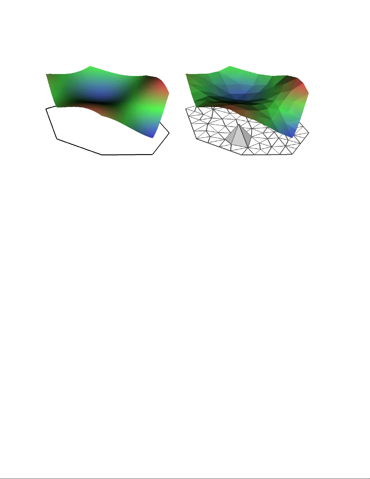
Think con tin uous: Mark o vian Gaussian mo dels in spatial statistics Daniel Simpson ∗ , Finn Lindgren & H ˚ av ard Rue Departmen t of Mathematical Sciences Norw egian Universit y of Science and T ec hnology N-7491 T rondheim, Norwa y No vem ber 27, 2024 Abstract Gaussian Mark ov random fields (GMRFs) are frequen tly used as computationally efficien t mo dels in spatial statistics. Unfortunately , it has traditionally b een difficult to link GMRFs with the more traditional Gaussian random field mo dels as the Marko v prop ert y is difficult to deplo y in contin uous space. F ollowing the pioneering work of Lindgren et al. (2011), we exp ound on the link b et ween Mark ovian Gaussian random fields and GMRFs. In particular, we discuss the theoretical and practical asp ects of fast computation with con tinuously specified Mark ovian Gaussian random fields, as w ell as the clear adv an tages they offer in terms of clear, parsimonious and in terpretable mo dels of anisotrop y and non-stationarity . 1 In tro duction F rom a practical viewpoint, the primary difficult y with spatial Gaussian mo dels in applied statistics is dimension, whic h t ypically scales with the num ber of observ ations. Computationally sp eaking, this is a disaster! It is, ho wev er, not a disaster unique to spatial statistics. Time s eries mo dels, for example, can suffer from the same problems. In the temp oral case, the ballo oning dimensionalit y is t ypically tamed b y adding a conditional indep endence, or Markovian , structure to the mo del. The k ey adv an tage of the Marko v property for time series mo dels is that the computational burden then gro ws only linearly (rather than cubically) in the dimension, which makes inference on these models feasible for long time series. Despite its success in time series mo delling, the Mark ov prop ert y has had a less exalted role in spatial statistics. Almost all instances where the Marko v prop ert y has b een used in spatial mo delling has b een in the form of Marko v random fields defined ov er a set of discrete lo cations connected by a graph. The most common Marko v random field models are Gaussian Marko v random fields (GMRFs), in which the v alue of the random field at the no des is join tly Gaussian (Rue and Held, 2005). GMRFs are typically written as x ∼ N ( µ , Q − 1 ) , where Q is the pr e cision matrix and the Mark ov prop ert y is equiv alen t to requiring that Q is sparse, that is Q ij = 0 iff x i and x j are conditionally independent (Rue and Held, 2005). As problems in spatial statistics are usually concerned with inferring a spatially contin uous effect o ver a domain of in terest, it is difficult to directly apply the fundamentally discrete GMRFs. F or this reason, it is commonly stated that there are tw o essen tial fields in spatial statistics: the one that uses ∗ Corresp onding author. Email: Daniel.Simpson@math.ntnu.no 1 GMRFs and the one that uses con tinuously indexed Gaussian random fields. In a recent read pap er, Lindgren et al. (2011) show ed that these tw o approaches are not distinct. By carefully utilising the con tinuous space Marko v prop ert y , it is p ossible to construct Gaussian random fields for which all quan tities of in terest can b e computed using GMRFs! The most exciting aspect of the Mark ovian mo dels of Lindgren et al. (2011) is their flexibility . There is no barrier—conceptual or computational—to extending them to construct non-stationary , anisotropic Gaussian random fields. F urthermore, it is even p ossible to construct them on the sphere and other manifolds. In fact, Simpson et al. (2011a) sho wed that there is essen tially no computational difference b et w een inferring a log-Gaussian Cox pro cess on a rectangular observ ation window and inferring one on a non-con vex, m ultiply connected region on the sphere! This type of flexibility is not found in an y other metho d for constructing Gaussian random field mo dels. In this pap er we carefully review the connections b et ween GMRFs, Gaussian random fields, the spatial Mark ov prop erty and deterministic approximation theory . It is hop ed that this will give the in terested reader some insigh t into the theory and practice of Marko vian Gaussian random fields. In Section 2 we briefly review the practical computational prop erties of GMRFs. Section 3 we take a detailed tour of the theory of Marko vian Gaussian random fields. W e b egin with a discussion of the spatial Marko v prop ert y and sho w how it naturally leads to differential op erators. W e then presen t a practical metho d for appro ximating Mark ovian Gaussian random fields and discuss what is mean b y a con tinuous approximation. In particular, we sho w that deterministic appro ximation theory can pro vide essen tial insights into the b eha viour of these approximations. W e then discuss some practical issues with choosing sets of basis functions b efore discussing extensions of the mo dels. Finally w e mention some further extensions of the method. 2 Practical computing with Gaussian Mark o v random fields Gaussian Marko v random fields p ossess tw o pleasant prop erties that make them useful for spatial problems: they facilitate fast computation for large problems, and they are quite stable with respect to conditioning. In this section w e will explore these tw o prop erties in the context of spatial statistics. 2.1 F ast computations with Gaussian Mark ov random fields As in the temp oral setting, the Marko vian prop ert y allows for fast computation of samples, likelihoo ds and other quan tities of in terest (Rue and Held, 2005). This allo ws the inv estigation of muc h larger mo dels than wou ld b e av ailable using general multiv ariate Gaussian mo dels. The situation is not, ho wev er, as go od as it is in the one dimensional case, where all of these quantities can b e computed using O ( n ) op erations, where n is the dimension of the GMRF. Instead, for the t wo dimensional spatial mo dels, samples and lik eliho o ds can b e computed in O ( n 3 / 2 ) op erations, which is still a significan t sa ving on the O ( n 3 ) op erations required for a general Gaussian mo del. A quick order calculation shows that computing a sample from an ˜ n –dimensional Gaussian random v ector without an y sp ecial structure tak es the same amount of time as computing a sample from GMRF of dimension n = ˜ n 2 ! The key ob ject when computing with GMRFs is the Cholesky decomp osition Q = LL T , where L is a lo wer triangular matrix. When Q is sparse, its Cholesky decomp osition can b e computed v ery efficien tly (see, for instance, Da vis, 2006). Once the Cholesky triangle has been computed, it is easy to sho w that x = µ + L − T z is a sample from the GMRF x ∼ N ( µ , Q − 1 ) where z ∼ N ( 0 , I ). Similarly , the log densit y for a GMRF can be computed as log π ( x ) = − n 2 log(2 π ) + n X i =1 log L ii − 1 2 ( x − µ ) T Q ( x − µ ) , 2 where L ii is the i th diagonal element of L and the inner product ( x − µ ) T Q ( x − µ ) can b e computed in O ( n ) calculations using the sparsity of Q . It is also p ossible to use the Cholesky triangle L to compute diag( Q − 1 ), which are the marginal v ariances of the GMRF (Rue and Martino, 2007). F urthermore, it is p ossible to sample from x conditioned on a smal l numb er of linear constraints x | B x = b , where B ∈ R k × n is usually a dense matrix and the n um b er of constraints, k , is v ery small. This o ccurs, for instance, when the GMRF is constrained to sum to zero. How ever, if one wishes to sample conditional on data, which usually corresp onds to a lar ge numb er of linear constrain ts, the metho ds in the next section are almost alw ays significan tly more efficient. While direct calculation of the conditional density is possible, when B is a dense matrix conditioning destroys the Marko v structure of the problem. It is still, ho w ever, p ossible to sample efficiently using a technique kno wn as c onditioning by Kriging (Rue and Held, 2005), whereb y an unconditional sample x is drawn from N ( µ , Q − 1 ) and then corrected using the equation x ∗ = x − Q − 1 B T ( B Q − 1 B T ) − 1 ( B x − b ) . When k is small, the conditioning by Kriging up date can b e computed efficiently from the Cholesky factorisation. W e reiterate, ho wev er, that when there are a large n umber of constrain ts, the conditioning b y Kriging metho d will b e inefficient, and, if B is sparse (as is the case when conditioning on data), it is usually better use the metho ds in the next subsection. An alternativ e metho d for conditional sampling can be constructed by noting that the conditioning b y Kriging up date x ∗ = x − δ x can b e computed by solving the augmen ted system  Q B T B 0   δ x y  =  0 B x − b  , (1) where y is an auxiliary v ariable. A standard application of Sylv ester’s inertia theorem (Theorem 8.1.17 in Golub and v an Loan, 1996) sho ws that the matrix in (1) is not p ositiv e definite, ho wev er the system can still b e solved using ordinary direct (or iterative) metho ds (Simpson et al., 2008). The augmented system (1) rev eals the geometric structure of conditioning by Kriging: augmen ted systems of equations of this form arise from the Karush-Kuhn-T uck er conditions in constrained optimisation (Benzi et al., 2005). In particular, the conditional sample solves the minimisation problem x ∗ = arg min x ∗ ∈ R n 1 2 k x ∗ − x k 2 Q sub ject to B x ∗ = b , where x is the unconditional sample and k y k 2 Q = y T Qy . That is, the conditional sample is the closest v ector that satisfies the linear constrain t to the unconditional sample when the distance is measured in the natural norm induced by the GMRF. The metho ds in this section are all predicated on the computation of a Cholesky factorisation. Ho wev er, for genuinely large problems, it ma y b e imp ossible to compute or store the Cholesky factor. With this in mind, a suite of metho ds were developed b y Simpson et al. (2007) b ased on mo dern iterative metho ds for solving sparse linear systems. These metho ds hav e shown some promise for large problems (Stric kland et al., 2011; Aune et al., 2011), although more work is needed on appro ximating the log densit y (Simpson, 2009; Aune and Simpson, 2011). 2.2 The effect of conditioning: fast Bay esian inference The second app ealing prop ert y of GMRFs is that they behav e well under conditioning. The discussion in this section is in timately tied to discretely specified GMRFs, ho w ever w e will see in Section 3.6 that 3 the formulation b elo w, and esp ecially the matrix A , has an imp ortan t role to pla y in the con tinuous setting. Consider the simple Ba yesian hierarc hical mo del y | x ∼ N ( Ax , Q − 1 y ) (2a) x ∼ N ( µ , Q − 1 x ) , (2b) where A , Q x and Q y are sparse matrices. A simple manipulation shows that ( x T , y T ) T is join tly a Gaussian Marko v random field with joint precision matrix Q xy =  Q x + A T Q y A − A T Q y − Q y A Q y  (3) and the mean defined implicitly through the equation Q xy µ xy =  Q x µ 0  . As ( x T , y T ) T is jointly a GMRF, it is easy to see (see, for example, Rue and Held, 2005) that x | y ∼ N  µ + ( Q x + A T Q y A ) − 1 A T Q y ( y − Aµ ) , ( Q x + A T Q y A ) − 1  . (4) It is imp ortan t to note that the precision matrices for the join t (3) and the conditional (4) distributions are only sparse—and the corresponding fields are only GMRFs—if A is sparse. This observ ation directly links the structure of the matrix A to the a v ailability of efficient inference metho ds and will b e imp ortan t in the coming sections. F or practical problems in spatial statistics, the mo del (2) is not enough: there will b e unkno wn parameters in b oth the lik eliho od and the laten t field. If w e group the unknown parameters in to a v ector θ , w e get the following hierarc hical model y | x , θ ∼ N ( Ax , Q y ( θ ) − 1 ) (5a) x | θ ∼ N ( µ , Q x ( θ ) − 1 ) (5b) θ ∼ π ( θ ) . (5c) In order to p erform inference on (5), it is common to use Mark ov c hain Mon te Carlo (MCMC) metho ds for sampling from the p osterior π ( x , θ | y ), ho w ever, this is not necessary . It’s an easy exercise in Gaussian densit y manipulation to show that the marginal p osterior for the parameters, denoted π ( θ | y ) can b e computed without in tegration and is giv en b y π ( θ | y ) ∝ π ( x , y | θ ) π ( θ ) π ( x | y , θ )     x = x ∗ , where x ∗ can b e an y point, but is typically tak en to b e the conditional mo de E ( x | y , θ ), and the corresp onding marginals π ( θ j | y ) can b e computed using numerical in tegration. Similarly , the marginals π ( x i | y ) can b e computed using n umerical in tegration and the observ ation that, for every θ , π ( x , y | θ ) is a GMRF (Rue and Martino, 2007; Rue et al., 2009). It follows that, for mo dels with Gaussian observ ations, it is p ossible to p erform deterministic in- ference that is exact up to the error in the n umerical integration. In particular, if there are only a mo derate n umber of parameters, this will b e extremely fast. F or non-Gaussian observ ation pro cesses, exact deterministic inference is no longer p ossible, ho w ever, Rue et al. (2009) sho wed that it is p ossible to construct extremely accurate approximate inference sc hemes by clev erly deplo ying a series of Laplace appro ximation. The in tegrated nested Laplace approximation (INLA) has b een used successfully on a large num b er of spatial problems (see, for example, F ong et al., 2010; Akerk ar et al., 2010; Sc hr¨ odle and Held, 2011; Riebler et al., 2011; Cameletti et al., 2011; Illian et al., 2011) and a user friendly R in terface is av ailable from http://r- inla.org . 4 In t r o B, W, M, & R SP DE/GMRF Exam ple End CA R Mat ´ er n Ma r k ov Whittle Th e c on ti n u ou s d om ai n Ma rk ov p rop e rt y S is a s epa rat ing s et fo r A and B : x ( A ) ⊥ x ( B ) | x ( S ) A S B Finn L indgren - finn. lindgren@math. ntnu. no Mat ´ er n /SP DE/GMRF Figure 1: An illustration of the spatial Mark ov prop ert y . If, for any appropriate set S , { x ( s ) : s ∈ A ) } is indep enden t of { x ( s ) : s ∈ B ) } given { x ( s ) : s ∈ S ) } , then the field x ( s ) has the spatial Marko v prop ert y . 3 Con tin uously sp ecified, Mark o vian Gaussian random fields One of the primary aims of spatial statistics is to infer a sp atial ly c ontinuous surface x ( s ) o ver the region of in terest. It is, therefore, necessary to build probabilit y distributions ov er the space of func- tions, and the standard wa y of doing this is to construct Gaussian random fields, which are the generalisation to functions of multiv ariate Gaussian distributions in the sense that for an y collec- tion of p oin ts ( s 1 , s 2 , . . . , s p ) T , the field ev aluated at those p oin ts is jointly Gaussian. In particular x ≡ ( x ( s 1 ) , x ( s 2 ) , . . . , x ( s p )) T ∼ N ( µ , Σ ), where the cov ariance matrix is giv en b y Σ ij = c ( s i , s j ) for some positive definite cov ariance function c ( · , · ). In most commonly used cases, the cov ariance function is non-zero ev erywhere and, as a result, Σ is a dense matrix. It is clear that we would lik e to transfer some of the pleasant computational prop erties of GMRFs, whic h are outlined ab o v e, to the Gaussian random field setting. The obvious barrier to this is that classical GMRF models are strongly tied to discrete sets of points, such as graphs (Rue and Held, 2005) and lattices (Besag, 1974). Throughout this section, we will discuss the recen t w ork of Lindgren et al. (2011) that has broken do wn the barrier b et w een GMRFs and spatially contin uous Gaussian random field mo dels. 3.1 The spatial Marko v prop erty F or temp oral pro cesses, defining the Mark ov property is greatly simplified b y the structure of time: its directional nature and the clear distinction b et w een past, present and future allo w for a v ery natural discussion of neighbourho o ds. Unfortunately , space is far less structured and, as such the Marko v prop ert y is harder to define exactly . In tuitively , ho wev er, the definition is generalised in an the ob vious w ay and is demonstrated by Figure 1. Informally , a Gaussian random field x ( s ) has the spatial Mark ov prop ert y if, for every appropriate set S separating A and B , the v alues of x ( s ) in A are conditionally indep enden t of the v alues in B given the v alues in S . A formal definition of the spatial Mark ov property can b e found in Rozano v (1977). It is not immediately ob vious how the spatial Mark ov prop ert y can b e used for computational 5 inference. Ho wev er, in an almost completely ignored pap er, Rozano v (1977) provided the vital c harac- terisation of Marko vian Gaussian random fields in terms of their p o wer spectra. The p o wer spectrum of a stationary Gaussian random field is defined as the F ourier transform of its cov ariance function c ( h ), that is R ( k ) ≡ 1 (2 π ) d Z R d exp( − i k T h ) c ( h ) . Rozano v sho w ed that a stationary field is Marko vian if and only if R ( k ) = 1 /p ( k ), where p ( k ) is a p ositiv e, symmetric polynomial. 3.2 F rom sp ectra to differen tial op erators While Rozano v’s characterisation of stationary Mark ovian random fields in terms of their p o w er sp ectra is elegan t, it is not ob vious ho w we can turn it in to a useful computational tool. The link comes from F ourier theory: there is a one-to-one corresp ondence b et ween p olynomials in the frequency space and differen tial op erators. T o see this, define the cov ariance op erator C of the Mark o vian Gaussian random field as the con volution C [ f ( · )]( h ) = Z R d c ( h 0 − s ) f ( h 0 ) d h 0 = Z R d exp( i k T h ) ˆ f ( k ) p ( k ) d k , where p ( k ) ≡ 1 /R ( k ) = P | i |≤ ` a i k i is a d –v ariate, p ositiv e, symmetric p olynomial of degree ` ; i = ( i 1 , . . . , i d ) T ∈ N d is a m ulti-index, meaning that k i = Q d l =1 k i l l and | i | = P d l =1 i l ; f ( · ) is a smo oth function that go es to zero rapidly at infinity; and ˆ f ( k ) is the F ourier transform of f ( h ). It follows from F ourier theory that the co v ariance op erator C has an in v erse, which w e will call the pr e cision op erator Q , and it is given b y Q [ f ( · )]( h ) ≡ C − 1 [ f ( · )]( h ) = Z R d exp( i k T h ) ˆ f ( k ) p ( k ) d k = X | i |≤ ` a i D i f ( h ) , where D l = i | l | ∂ | l | ∂ h l 1 1 ∂ h l 2 2 · ∂ h l d d are the appropriate m ultiv ariate deriv ativ es. The follo wing prop osition summarises the previous discussion and sp ecialises the result to isotropic fields. Prop osition 1. A stationary Gaussian r andom field x ( s ) define d on R d is Markovian if and only if its c ovarianc e op er ator C [ f ( · )] has an inverse of the form Q [ f ( · )]( h ) = X | i |≤ ` a i D i f ( h ) , wher e a i ar e the c o efficients of a r e al, symmetric p olynomial p ( k ) = P | i |≤ ` a i k i . F urthermor e, x ( s ) is isotr opic if and only if Q [ f ( · )]( h ) = ` X i =0 ˜ a i ( − ∆) i f ( h ) , wher e ∆ = P d i =1 ∂ 2 ∂ h 2 i is the d -dimensional L aplacian and ˜ p ( t ) = P ` i =0 ˜ a i t i is a r e al, symmetric univariate p olynomial. 6 The critical p oin t of the ab o v e paragraph is that for Marko vian Gaussian random fields, the co- v ariance is the inv erse of a lo c al op erator, in the sense that the v alue of Q [ f ( · )]( h ) only dep ends on the v alue of f ( h ) in an infinitesimal neighbourho o d of h . This is in stark con trast to the cov ariance op erator, which is an integral op erator and therefore dep ends on the v alue of f ( h ) ev erywhere that the co v ariance function is non-zero. It is this lo calit y that will lead us to GMRFs and the promised land of sparse precision matrices and fast computations. 3.3 Sto c hastic differen tial equations and Mat´ ern fields The discussion in the previous subsection ga ve a very general form of Mark ovian Gaussian random fields. In this section we will, for the sake of sanit y , simplify the setting greatly . Consider the sto chastic partial differential (SPDE) ( κ 2 − ∆) α/ 2 x ( s ) = W ( s ) , (6) where W ( s ) is Gaussian white noise and α > 0. The solution to the SPDE will b e a Gaussian random field and some formal manipulations (made precise b y Rozano v, 1977) show that the precision op erator is Q = [ E ( xx ∗ )] − 1 = h ( κ 2 − ∆) − α/ 2 E ( W W ∗ )( κ 2 − ∆) − α/ 2 i − 1 = ( κ 2 − ∆) α . It follows that Q is a lo cal differen tial operator when α is an in teger and, by Prop osition 1, the stationary solution to (6) for integer α is a Mark ovian Gaussian random field. Somewhat surprisingly , we ha ve no w ven tured bac k into the more common parts of spatial statistics: Whittle (1954, 1963) sho wed that, for an y α > d/ 2, the solution to (6) has a Mat ´ ern co v ariance function. That Mat´ ern family of cov ariance functions, whic h is giv en by c σ 2 ,ν,κ ( h ) = σ 2 2 ν − 1 Γ( ν ) ( κ k h k ) ν K ν ( κ k h k ) , where σ 2 is the v ariance parameter, κ controls the range, and ν = α − d/ 2 > 0 is the shap e parameter, is one of the most widely used families of stationary , isotropic co v ariance functions. The results of the previous section sho w that, when ν + d/ 2 is an in teger, the Mat ´ ern fields are Marko vian. 3.4 Appro ximating Gaussian random fields: the finite element metho d Ha ving no w laid all of the theoretical groundw ork, we can consider the fundamental question in this pap er: how do can we use GMRFs to appro ximate a Gaussian random field? In order to construct a go o d approximation, it is vital to remember that ev ery realisation of a Gaussian random field is a function . It follo ws that any sensible metho d for approximating Gaussian random fields is necessarily connected to a metho d for approximating an appropriate class of deterministic functions. Therefore, follo wing Lindgren et al. (2011), w e are on the h unt for simple metho ds for appro ximating functions. A reasonably simple metho d for appro ximating contin uous functions is demonstrated in Figure 2, whic h shows a piecewise linear approximation to a deterministic function f ( s ) that is defined ov er a triangulation of the domain. This appro ximation is of the form f ( s ) ≈ f h ( s ) = n X i =1 w i φ i ( s ) , 7 (a) A contin uous function (b) A piecewise linear approximation Figure 2: Piecewise linear appro ximation of a function ov er a triangulated mesh. where the basis function φ i ( s ) is the piecewise linear function that is equal to one at the i th vertex of the mesh and is zero at all other vertices and the subscript h denotes the largest triangle edge in the mesh and is used to differentiate b etw een piecewise linear functions o v er a mesh and general functions. The grey pyramid in Figure 2 is an example of a basis function. With this in hand, we can define a piecewise linear Gaussian random field as x h ( s ) = n X i =1 w i φ i ( s ) , (7) where φ i ( s ) are as b efore and the w eigh ts w are now join tly a Gaussian random vector. Our aim is no w to find the statistical properties of w that make x h ( s ) approximate the Mark ovian Mat ´ ern fields. In order to do this, we use the c haracterisation of a Mat ´ ern field as the stationary solution to (6). F or simplicit y , let us consider α = 2 on a domain Ω ⊂ R 2 . An y solution of (6) also satisfies, for an y suitable function ψ ( s ), Z Ω ψ ( s )( κ 2 − ∆) x ( s ) ds = Z Ω ψ ( s ) W ( ds ) and an application of Green’s form ula leads to Z Ω κ 2 ψ ( s ) x ( s ) + ∇ ψ ( s ) · ∇ x ( s ) dx = Z Ω ψ ( s ) W ( ds ) , (8) where the in tegrals on the righ t hand sides are integrals with resp ect to white nose (see Chapter 5 of Adler and T a ylor, 2007) and the second line follows from Green’s form ula and the (new) condition that the normal deriv ative of x ( s ) v anishes on the b oundary of Ω. F urthermore, if w e find x ( s ) such that (8) holds for any sensible ψ ( s ), then x ( s ) is the w eak solution to (6) and it can b e shown that it is a Gaussian random field with the appropriate Mat ´ ern cov ariance function. Unfortunately , w e cannot test (8) against every function ψ ( s ), so we will instead c hose a finite set { ψ j ( s ) } n j =1 to test against. Substituting x h ( s ) in to (8) and testing against this set of ψ j s, we get the 8 system of linear equations n X i =1  κ 2 Z Ω ψ j ( s ) φ i ( s ) ds + Z Ω ∇ ψ j ( s ) · ∇ φ i ( s ) ds  w i = Z Ω ψ j ( s ) dW ( s ) , j = 1 , . . . , n. (9) Finally , we c hose our test functions ψ j ( s ) to be the same as our basis functions φ i ( s ) and arriv e at the Galerkin finite elemen t method. F or piecewise linear functions o v er a triangular mesh, it is easy to compute all of the in tegrals on the left hand side of (9). The white noise in tegral on the right hand side can b e computed and it is Gaussian with mean zero and Co v  Z Ω φ i ( s ) dW ( s ) , Z Ω φ j ( s ) dW ( s )  = Z Ω φ i ( s ) φ j ( s ) ds. (10) W e can, therefore write (9) in matrix form as K ˜ w ∼ N ( 0 , ˜ C ) , where K = κ ˜ C + G and the matrices are giv en by ˜ C ij = R Ω φ i ( s ) φ j ( s ) ds and G ij = R Ω ∇ ψ j ( s ) ·∇ φ i ( s ) ds . A quic k lo ok at the definitions of ˜ C and G shows that, due to the highly lo cal nature of the basis functions, these matrices are sparse. Unfortunately , ˜ C − 1 is a dense matrix and, therefore ˜ w will not b e a GMRF. Ho w ever, replacing ˜ C by the diagonal matrix C = diag( R Ω φ i ( s ) ds, i = 1 , . . . , n ) gives essen tially the same result numerically (Bolin and Lindgren, 2009) and can be shown not to increase the rate of conv ergence of the appro ximation (App endix C.5 of Lindgren et al., 2011). Using C , it follows that the solution to K w ∼ N ( 0 , ˜ C ) is a GMRF with zero mean and sparse precision matrix Q = K T C K . The GMRFs that corresp ond to other integer v alues of α can be found in Lindgren et al. (2011). 3.5 A con tin uous appro ximation to a con tin uous random field W e hav e now derived a GMRF w from the contin uous Mat´ ern field x ( s ). It is, therefore, reasonable to w onder how w ell w approximates x ( s ). It do esn ’t! The GMRF w w as defined as the w eigh ts of a basis function expansion (7) and only mak e sense in this con text. In particular, w is not trying to approximate x ( s ) at the mesh vertices. Instead, the piecewise linear Gaussian random field x h ( s ) = P n i =1 w i φ i ( s ) tries to appro ximate the true random field everywher e . Because of the nature of this contin uous ap- pro ximation, x h ( s ) will necessarily ov erestimate the v ariance at the vertices and underestimate in in the centre of the triangles. One of the real adv antages of using piecewise linear basis functions is that a lot of w ork has gone into w orking out their appro ximation properties (Brenner and Scott, 2007). W e can lev erage this information to get hard b ounds on the con vergence of x h ( s ) to x ( s ). The follo wing theorem is a simple example of this t yp e of result. It shows that functionals of b oth the field and its deriv ativ e conv erge to the true functionals and the error is O ( h ), where h is the length of the largest edge in the mesh. The theorem also links the con v ergence of functionals of the random field to how w ell the piecewise linear basis functions can approximate functions in the Sobolev space H 1 , which consists of square in tegrable functions f ( s ) for which k f k 2 H 1 = κ 2 R Ω f ( s ) 2 ds + R Ω ∇ f ( s ) · ∇ f ( s ) ds is finite. Theorem 1. L et L = κ 2 − ∆ . Then, for any f ∈ H 1 , E  Z Ω f ( s ) L ( x ( s ) − x h ( s )) ds  2 ≤ ch 2 k f k 2 H 1 , wher e c is a c onstant and h is the size of the lar gest triangle e dge in the mesh. 9 Pr o of. Let f ∈ H 1 , f h ( s ) be the H 1 –pro jection of f onto the finite elemen t space V h = span { φ 1 ( s ) , . . . , φ n ( s ) } , that is let f h b e the solution to min f h ∈ V h k f − f h k H 1 . It follows that Z Ω f ( s ) Lx h ( s ) ds = Z Ω ( f ( s ) − f h ( s )) Lx h ( s ) ds + Z Ω f h ( s ) Lx h ( s ) ds = Z Ω f h ( s ) Lx h ( s ) dx = Z Ω f h ( s ) dW ( s ) , where the second equalit y follows from the Galerkin prop erty of x h ( s ) (Brenner and Scott, 2007), which states that R Ω g ( s ) Lx h ( s ) ds = 0 whenev er g ( s ) is in the orthogonal complement of V h with resp ect to the H 1 inner pro duct. It follo ws directly that Z Ω f ( s ) L ( x ( s ) − x h ( s )) ds = Z Ω ( f ( s ) − f h ( s )) dW ( s ) . Therefore, it follo ws from the prop erties of white noise in tegrals that E  Z Ω f ( s ) L ( x ( s ) − x h ( s )) ds  2 = E  Z Ω ( f ( s ) − f h ( s )) dW ( s )  2 = Z Ω ( f ( s ) − f h ( s )) 2 ds. It follows from Theorem 4.4.20 in Brenner and Scott (2007) that (under some suitable assumptions on the triangulation) k f n − f k L 2 (Ω) ≤ ch k f k H 1 . The k ey lesson from the proof of Theorem 1 is that the conv ergence of functionals of x h ( s ) depends solely on ho w w ell the basis functions can approximate a fixed H 1 function. Therefore, it is vital to consider the appro ximation prop erties of y our basis functions! 3.6 Cho osing basis functions: don’t forget ab out A While w e ha ve computed ev erything with respect to piecewise linear functions, the metho ds considered ab o v e w ork for an y set of test and basis functions for whic h all of the computations mak e sense. How ever, w e strongly warn against using an y of the more esoteric choices. There are tw o main issues that can app ear. The first issue is that the wrong choice of basis functions will destroy the Marko v structure of the p osterior mo del, whic h will annihilate the computational gains we hav e work ed so hard for. The second issue, which is related to Theorem 1 is muc h more problematic: not all sets of basis functions will provide go od appro ximations to x ( s ). In Section 2.2, we lo oked at the GMRF computations for hierarc hical Gaussian mo dels. Consider a simple Gaussian observ ation pro cess of the form y i ∼ N ( x h ( s i ) , σ 2 ) , i = 1 , . . . , N 10 − 0 . 3 − 0 . 2 − 0 . 1 0 0 . 1 0 . 2 0 . 3 0 1 2 · 10 − 2 F i gu r e 1: A c om p ar i s on of t h e s t an d ar d k e r n e l f u n c t i on ( s ol i d l i n e s ) an d t h e s m o ot h e d k e r n e l f u n c t i on ( d ot t e d l i n e s ) f or α =2 ( η =1 / 2) an d κ = 20. 0 0 . 2 0 . 4 0 . 6 0 . 8 1 0 . 8 1 1 . 2 Appro ximation e rr or Kernel Smo oth Kernel GMRF F i gu r e 2: T h i s fi gu r e s h o w s t h e e r r or i n t h e ap p r o x i m at i on s t o x ( s ) ≡ 1 f or al l t h r e e s e t s of b as i s f u n c t i on s f or α = 2 an d κ = 20. T h e d as h - d ot t e d l i n e s h o w s t h e s i m p l e k e r n e l ap p r o x i m at i on . T h e s m o ot h e d k e r n e l ap p r o x i m at i on ( s ol i d l i n e ) b e h a v e s m u c h b e t t e r , al t h ou gh i t d o e s d e m on s t r at e e d ge e ff ects. The fin ite e l e m e n t b as i s u s e d f or t h e G M R F r e p r e s e n t at i on of t h e S P D E ( d as h e d l i n e ) , w h i c h i s d i s c u s s e d i n t h e n e x t s e c t i on , r e p r o d u c e s c on s t an t f u n c t i on s e x ac t l y . 2 Figure 3: T ak en from (Simpson et al., 2011b). The error in the b est appro ximation to x ( s ) = 1, s ∈ [0 , 1]. The dotted line is the na ¨ ıv e k ernel basis, while the solid line is an integrated kernel basis deriv ed by Simpson et al. (2011b). The piecewise linear basis (dashed line) reproduces the function exactly . where the num b er of data p oin ts N do es not need to b e related to the num b er of mesh vertices n . It follo ws that the datap oin t ( s i , y i ) requires the computation of the sum P n j =1 w j φ j ( s i ). When the basis functions are lo cal, there are only a few non-zero terms in this sum and the corresp onding matrix A , whic h has en tries A ij = φ j ( s i ), is sparse. F or piecewise linear functions on a triangular mesh, eac h row of A has at most 3 non-zero entries. On the other hand, consider a basis consisting of the first n functions from the Karhunen-Lo ´ ev e expansion of x ( s ). In this case, it’s easy to sho w that the precision matrix for w will be diagonal. Unfortunately , these basis function are usually non-zero ev erywhere, so A will b e a completely dense N × n matrix, whic h, for large datasets will b ecome the dominant computational cost. The appro ximation prop erties of sets of basis functions are t ypically very hard to determine. There are, how ev er, some go o d guiding principles. The first principle is that your basis functions should do a go od job approximating simple functions. Y ou usually wan t to b e able to at least appro ximate constan t and linear functions well. A second guiding principle is that y ou should b e v ery careful when y our basis functions dep end on a parameter that is b eing estimated. It is imp ortan t to chec k that the appro ximation is still sensible ov er the entire parameter range. Figure 3 is an example of this problem, tak en from Simpson et al. (2011b), sho ws the b est approximation to a constan t function using the basis deriv ed from a con volution k ernel approximation to a one dimensional Mat´ ern field with ν = 3 / 2 and κ = 20. The basis functions are computed with resp ect to a fixed grid of 11 equally spaced knots s i , i = 1 , . . . , 11 and are giv en b y φ i ( s ) = 1 (2 π ) 1 / 2 κ exp( − κ | s − s i | ) . When κ gets large, the basis functions get sharper and the approximation gets worse. At its w orst, the effectiv e range of the k ernel b ecomes shorter than grid of knots. Therefore, if κ b ecomes large relative to the grid spacing, b oth Kriging estimates and v ariance estimates will b e badly infected by the p oor c hoice of basis function. On the other hand, it can be sho wn that piecewise linear Galerkin finite elemen t appro ximations are stable in the sense that the norm of the approximation can b e b ounded ab o ve b y 11 (a) A sample from an anisotropic field (b) The cov ariance functions Figure 4: An anisotropic field defined through (6) when the Laplacian is replace with the anisotropic v ariant ∇ · ( D ( s ) ∇ ( τ x ( s ))). The right hand figure sho ws the approximate co v ariance function ev aluated at three points and the non-stationarit y is eviden t. an appropriate norm of the true solution. This means that a piecewise linear basis, when used in this w ay , will never display this bad behaviour. Another consideration when choosing sets of basis functions is the smoothness of the random field. Theorem 1 directly links the con vergence of the appro ximate fields to how w ell the basis functions can appro ximate a certain class of functions. This will usually b e the case. Typically , the smoother the field is, the more useful higher order “spectral” bases will b e. F or a smo oth enough field, it ma y actually b e c heap er to use a small, w ell chosen global basis than a large basis full of local functions. 3.7 Extending the mo dels: anisotropy , drift, and space-time mo dels on manifolds One of the main adv an tages to the SPDE formulation is that it is easy to construct non-stationary v ariants. Non-stationary fields can no w b e defined b y letting the parameters in (6), b e space-dependent. F or example, log κ can b e expanded using a few weigh ted smo oth basis functions log κ ( s ) = X i β i b i ( s ) (11) and similar expansions can b e used for τ . This extension requires only minimal changes to the method used in the stationary case. More interestingly , w e can also incorp orate mo dels of spatially v arying anisotrop y b y replacing the Laplacian ∆ in (6) with the more general op erator ∇ · ( D ( s ) ∇ ( τ x ( s ))) ≡ 2 X i,j =1 ∂ ∂ s i  D ij ( s ) ∂ ∂ s j ( τ ( s ) x ( s ))  . These models can be extended ev en farther by incorp orating a “drift” term, as w ell as temp oral depen- dence, which leads to the general mo del ∂ ∂ t ( τ u ( s, t )) + ( κ 2 ( τ x ( s, t )) − ∇ · ( D ∇ ( τ x ( s, t )))) + b · ∇ ( τ x ( s, t )) = W ( s, t ) , (12) where t is the time v ariable and b is a vector describing the direction of the drift and the dependence of κ , τ , D and b on s and t has b een suppressed. The concepts behind the construction of Marko vian appro ximations to the stationary SPDE transfer almost completely to this general setting, how ever more care needs to b e taken with the exact form of the discretisation (F uglstad, 2010). 12 Figure 5: A sample from a non-stationary , anisotropic random field on the sphere. A strong adv antage of defining non-stationarit y through (12) is that the underlying ph ysics is w ell understo od. F or example the second order term ∇ · ( D ∇ ( τ x ( s, t )))) describ es the diffusion, where the matrix D ( s, t ) describ es the preferred direction of diffusion at lo cation s and time t . A spatial random field with a non-constan t diffusion matrix D ( s ) is shown in Figure 4. Similarly , the first order term b · ∇ ( τ x ( s, t )) describ es an advection effect and b ( s, t ) can b e in terpreted as the direction of the forcing field. W e note that unlik e other metho ds for mo delling non-stationarity , the parametrisation in this mo del is unc onstr aine d . This is in con trast to the deformation metho ds of Sampson and Guttorp (1992), in whic h the deformation must b e constrained to b e one-to-one. Initial work on parameterising and p erforming inference on these mo dels has b een undertaken b y F uglstad (2011). An in teresting consequence of defining our mo dels through lo c al sto chastic partial differen tial equa- tions, suc h as (12), is that the SPDEs still mak e sense when R d is replaced by a space that is only lo cally flat. W e can, therefore, use (12) to define non-stationary Gaussian fields on manifolds, and still obtain a GMRF representation. F urthermore, the computations can b e done in essentially the same w ay , the only change is that the Gaussian noise is no w a Gaussian random measure, and that w e need to take in to accoun t the local curv ature when computing the in tegrals to obtain the solution. Figure 5 sho ws a realisation of a non-stationary Gaussian random field on a sphere, with a mo del similar to the one used in Figure 4. The solution is still explicit, so all elements of the precision matrix, for a fixed triangularisation, can b e directly computed with no extra cost. The abilit y to construct computationally efficien t representations of non-stationary random fields on a manifold is imp ortan t, for example, when mo delling en vironmental data on the sphere. 3.8 F urther extensions: areal data, m ultiv ariate random fields and non-in teger α s The com bination of a contin uously sp ecified approximate random field and a Mark ovian structure allo ws for the straightforw ard assimilation of areal and point-referenced data. The trick is to utilise the matrix A in the observ ation equation (5a). The link betw een the latent GMRF and the point-referenced data is as describ ed ab o ve. F or the areal data, the dependence is through in tegrals of the random field and these in tegrals can b e computed exactly for x h ( s ) and the resulting sums go into A . If a more complicated functional of the random field has b een observ ed, this can b e appro ximated using n umerical quadrature. This has been recen tly applied b y Simpson et al. (2011a) to inferring log-Gaussian p oin t pro cesses. It is also p ossible to extend the SPDE framework considered ab o ve to a multiv ariate setting. Pri- marily , the idea is to replace a single SPDE with a system of SPDEs. It can be shown (w ork in progress) 13 that these mo dels ov erlap with, but are not equiv alen t to, the m ultiv ariate Mat ´ ern mo dels constructed b y Gneiting et al. (2010). The only Mark ovian Mat ´ ern mo dels are those where the smo othing parameter is d/ 2 less than an in teger. It turns out, how ev er, that w e can construct go od Mark ov random field approximations when α isn’t an in teger (see the authors’ resp onse in Lindgren et al., 2011). This is essen tially a p ow erful extension of the GMRF approximations of Rue and Tjelmeland (2002). W e are currently working on appro ximating non-Mat ´ ern random fields using this metho d. 4 Conclusion In this pap er we hav e surv eyed the deep and fascinating link b et ween the contin uous Mark ov property and computationally efficien t inference. The material in this pap er barely scratc hes the surface of the questions, applications and o ddities of these fields (for instance, Bolin (2011) uses a similar construction for non-Gaussian noise pro cesses). How ever, we ha ve demonstrated that by carefully considering the Mark ov prop ert y , w e are able to greatly bo ost our mo delling capabilities while at the same time ensuring that the models are fast to compute with. The combination of flexible modelling and fast computations ensures that inv estigations into Mark o vian random fields will con tinue to pro duce in teresting and useful results well in to the future. References R. J. Adler and J. T a ylor. R andom Fields and Ge ometry . Springer Monographs in Mathematics. Springer, 2007. R. Akerk ar, S. Martino, and H. Rue. Approximate ba y esian inference for surviv al mo dels. Sc andinavian Journal of Statistics , 28(3):514–528, 2010. E. Aune and D. P . Simpson. Hyper-parameter estimation inv olving high dimensional gaussian distribu- tions. In ISI 2011 , 2011. E. Aune, J. Eidsvik, and Y. P okem. Iterative n umerical metho ds for sampling from high dimensional gaussian distributions. T echnical Rep ort 4/2011, NTNU, 2011. M. Benzi, G. Golub, and J. Liesen. Numerical solutions of saddle p oint problems. A cta Numeric a , 14: 1–137, 2005. J. Besag. Spatial in teraction and the statistical analysis of lattice systems (with discussion). Journal of the R oyal Statistic al So ciety, Series B , 36(2):192–225, 1974. D. Boli n. Spatial Mat ´ ern fields driv en b y non-Gaussian noise. T echnical Rep ort 2011:4, Lund Univ ersit y , 2011. D. Bolin and F. Lindgren. W a velet Marko v mo dels as efficient alternatives to tap ering and con volution fields. T ec hnical Report 2009:13, Lund Universit y , 2009. S. C. Brenner and R. Scott. The Mathematic al The ory of Finite Element Metho ds . Springer, 3rd edition, 2007. M. Cameletti, F. Lindgren, D. P . Simpson, and H. Rue. Spatio-temporal mo delling of particulate matter concen tration through the SPDE approac h. AStA A dv Stat Anal , Submitted, 2011. 14 T. A. Davis. Dir e ct metho ds for sp arse line ar systems . SIAM Bo ok Series on the F undamentals of Algortihms. SIAM, Philadelphia, 2006. Y. F ong, H. Rue, and J. W ak efield. Bay esian inference for generalized linear mixed models. Biometrics , 11(3):397–412, 2010. G.-A. F uglstad. Approximating Solutions of Sto chastic Differential Equations with Gaussian Mark ov Random Fields. Pre-Master’s thesis, Departmen t of Mathematical Sciences, NTNU, 2010. G.-A. F uglstad. Spatial Mo delling and Inference with SPDE-based GMRFs. Master’s thesis, Department of Mathematical Sciences, NTNU, 2011. T. Gneiting, W. Kleiber, and M. Schlather. Mat´ ern cross-cov ariance functions for m ultiv ariate random fields. Journal of the A meric an Statistic al Asso ciation , 105(491):1167–1177, 2010. G. H. Golub and C. F. v an Loan. Matrix Computations . Johns Hopkins Univ ersity Press, Baltimore, 3rd edition, 1996. J. B. Illian, S. H. Sørby e, and H. Rue. A toolb ox for fitting complex spatial point pro cess mo dels using in tegrated Laplace transformation (INLA). submitte d , 2011. F. Lindgren, H. Rue, and J. Lindstr¨ om. An explicit link b et ween Gaussian fields and Gaussian Mark ov random fields: The stochastic partial differen tial equation approac h (with discussion). Journal of the R oyal Statistic al So ciety. Series B. Statistic al Metho dolo gy , 73(4):423–498, September 2011. A. Riebler, L. Held, and H. Rue. Gender-sp ecific differences and the impact of family in tegration on time trends in age-stratified swiss suicide rates. A nnals of Applie d Statistics , Accepted, 2011. J. A. Rozanov. Mark ov random fields and sto c hastic partial differential equations. Math. USSR Sb. , 32 (4):515–534, 1977. H. Rue and L. Held. Gaussian Markov R andom Fields: The ory and Applic ations , v olume 104 of Mono- gr aphs on Statistics and Applie d Pr ob ability . Chapman & Hall, London, 2005. H. Rue and S. Martino. Appro ximate Ba yesian inference for hierarc hical Gaussian Marko v random fields mo dels. Journal of Statistic al Planning and Infer enc e , 137(10):3177–3192, 2007. Sp ecial Issue: Ba yesian Inference for Stochastic Pro cesses. H. Rue and H. Tjelmeland. Fitting Gaussian Marko v random fields to Gaussian fields. Sc andinavian Journal of Statistics , 29(1):31–50, 2002. H. Rue, S. Martino, and N. Chopin. Appro ximate Bay esian inference for latent Gaussian models using in tegrated nested Laplace appro ximations (with discussion). Journal of the R oyal Statistic al So ciety, Series B , 71(2):319–392, 2009. P . D. Sampson and P . Guttorp. Nonparametric estimation of nonstationary spatial cov ariance structure. Journal of the A meric an Statistic al Asso ciation , 87(417):108–119, 1992. B. Sc hr¨ odle and L. Held. Spatio-temp oral disease mapping using INLA. Envir onmetrics , 22(6):725–734, Septem b er 2011. D. P . Simpson. Krylov subsp ac e metho ds for appr oximating functions of symmetric p ositive definite matric es with applic ations to applie d statistics and anomalous diffusion . PhD thesis, Queensland Univ ersity of T ec hnology , 2009. 15 D. P . Simpson, I. T urner, and A. Pettitt. F ast sampling from a Gaussian Marko v random field using Krylo v subspace approac hes. T echnical rep ort, Queensland Universit y of T ec hnology , 2007. D. P . Simpson, I. W. T urner, and A. N. P ettitt. Sampling from Gaussian Marko v random fields conditioned on linear constraints. ANZIAM J (CT AC 2006) , 48:C1041–C1053, July 2008. http: //anziamj.austms.org.au/ojs/index.php/ANZIAMJ/article/view/131 [July 17, 2008]. D. P . Simpson, J. Illian, F. Lindgren, S. Sørby e, and H. Rue. Computationally efficien t inference for log-Gaussian Cox pro cesses. Submitte d , 2011a. D. P . Simpson, F. Lindgren, and H. Rue. In order to mak e spatial statistics computationally feasible, w e need to forget about the cov ariance function. Envir onmetrics , Accepted, 2011b. C. M. Stric kland, D. P . Simpson, I. W. T urner, r. Denham, and K. L. Mengersen. F ast Ba yesian analysis of spatial dynamic factor mo dels for multitemporal remotely sensed imagery . Journal of the R oyal Statistic al So ciety : Series C , 60(1):109–124, Jan uary 2011. P . Whittle. On stationary pro cesses in the plane. Biometrika , 41(3/4):434–449, 1954. P . Whittle. Sto c hastic processes in several dimensions. Bul l. Inst. Internat. Statist. , 40:974–994, 1963. 16