NIFTY - Numerical Information Field Theory - a versatile Python library for signal inference

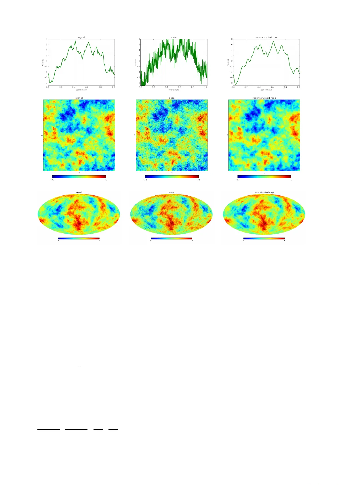
Astronom y & Astroph ysics man uscript no. NIFTY c  ESO 2018 No v em b er 1, 2018 NIFT Y ? – Numerical Info rmation Field Theo ry a versatile P YTHON lib ra ry for signal inference Marco Selig 1 , Mic hael R. Bell 1 , Henrik Junklewitz 1 , Niels Opp ermann 1 , Martin Reinec k e 1 , Maksim Greiner 1 2 , Carlos P ac ha joa 1 3 , and T orsten A. Enßlin 1 1 Max Planc k Institute für Astrophysik (Karl-Sch warzsc hild-Straße 1, D-85748 Garc hing, German y) 2 Ludwig-Maximilians-Univ ersität München (Gesch wister-Scholl-Platz 1, D-80539 München, German y) 3 T echnisc he Univ ersität Münc hen (Arcisstraße 21, D-80333 Münc hen, German y) Receiv ed 05 F eb. 2013 / Accepted 12 Apr. 2013 ABSTRA CT NIFTy , “Numerical Information Field Theory”, is a softw are pack age designed to enable the developmen t of signal inference algorithms that operate regardless of the underlying spatial grid and its resolution. Its ob ject-orien ted frame- w ork is written in Python , although it accesses libraries written in Cython , C++, and C for efficiency . NIFTy offers a to olkit that abstracts discretized representations of contin uous spaces, fields in these spaces, and operators acting on fields into classes. Thereby , the correct normalization of op erations on fields is taken care of automatically without concerning the user. This allows for an abstract formulation and programming of inference algorithms, including those deriv ed within information field theory . Thus, NIFTy p ermits its user to rapidly prototype algorithms in 1D, and then apply the developed co de in higher-dimensional settings of real world problems. The set of spaces on which NIFTy op erates comprises point sets, n -dimensional regular grids, spherical spaces, their harmonic counterparts, and product spaces constructed as combinations of those. The functionalit y and diversit y of the pack age is demonstrated b y a Wiener filter co de example that successfully runs without mo dification regardless of the space on whic h the inference problem is defined. Key w ords. metho ds: data analysis – methods: n umerical – metho ds: statistical – techniques: image processing 1. Intro duction In many signal inference problems, one tries to reconstruct a con tin uous signal field from a finite set of experimen- tal data. The finiteness of data sets is due to their incom- pleteness, resolution, and the sheer duration of the experi- men t. A further complication is the inevitability of experi- men tal noise, which can arise from v arious origins. Numer- ous metho dological approaches to such inference problems are kno wn in mo dern information theory founded b y Co x (1946); Shannon (1948); Wiener (1949). Signal inference metho ds are commonly formulated in an abstract, mathematical wa y to b e applicable in v arious scenarios; i.e., the metho d itself is indep endent, or at least partially independent, of resolution, geometry , physical size, or even dimensionality of the inference problem. It then is up to the user to apply the appropriate metho d correctly to the problem at hand. In practice, signal inference problems are solved numeri- cally , rather than analytically . Numerical algorithms should try to preserv e as m uch of the universalit y of the under- lying inference metho d as possible, giv en the limitations of a computer en vironmen t, so that the co de is reuseable. F or example, an inference algorithm developed in astro- ph ysics that reconstructs the photon flux on the sky from ? NIFTy homepage http://www.mpa- garching.mpg.de/ ift/nifty/ ; Excerpts of this paper are part of the NIFTy source co de and do cumentation. high energy photon coun ts migh t also serve the purpose of reconstructing tw o- or three-dimensional medical images obtained from tomographical X-rays. The desire for multi- purp ose, problem-indep endent inference algorithms is one motiv ation for the NIFTy pack age presented here. Another is to facilitate the implemen tation of problem specific algo- rithms b y providing many of the essen tial operations in a con v enien t w a y . NIFTy stands for “Numerical Information Field The- ory”. It is a softw are pack age written in Python 1 2 , how- ev er, it also incorp orates Cython 3 (Behnel et al. 2009; Sel- jeb otn 2009), C++, and C libraries for efficien t computing. The purp ose of the NIFTy library is to provide a to olkit that enables users to implemen t their algorithms as ab- stractly as they are formulated mathematically . NIFTy ’s field of application is kept broad and not bound to one sp ecific metho dology . The implementation of maximum en- trop y (Jaynes 1957, 1989), likelihoo d-free, maxim um lik e- liho o d, or full Bay esian inference metho ds (Bay es 1763; Laplace 1795/1951; Co x 1946) are feasible, as w ell as the implemen tation of p osterior sampling pro cedures based on Mark o v chain Monte Carlo pro cedures (Metrop olis & Ulam 1949; Metrop olis et al. 1953). 1 Python homepage http://www.python.org/ 2 NIFTy is written in Python 2 whic h is supp orted b y all platforms and compatible to existing third party pack ages. A Python 3 complian t v ersion is left for a future upgrade. 3 Cython homepage http://cython.org/ Article num b er, page 1 of 10 A&A pro ofs: man uscript no. NIFTY Although NIFTy is v ersatile, the original inten tion was the implementation of inference algorithms that are formu- lated metho dically in the language of information field the- ory 4 (IFT). The idea of IFT is to apply information theory to the problem of signal field inference, where “field” is the ph ysicist’s term for a contin uous function ov er a contin uous space. The recov ery of a field that has an infinite n um b er of degrees of freedom from finite data can b e ac hiev ed by exploiting the spatial contin uity of fields and their internal correlation structures. The framew ork of IFT is detailed in the w ork b y Enßlin et al. (2009) where the focus lies on a field theoretical approac h to inference problems based on F eynman diagrams. An alternative approach using en- tropic matching based on the formalism of the Gibbs free energy can b e found in the w ork b y Enßlin & W eig (2010). IFT based metho ds hav e b een developed to reconstruct sig- nal fields without a priori knowledge of signal and noise correlation structures (Enßlin & F rommert 2011; Opp er- mann et al. 2011). F urthermore, IFT has b een applied to a n um b er of problems in astroph ysics, namely to recov er the large scale structure in the cosmic matter distribution us- ing galaxy counts (Kitaura e t al. 2009; Jasc he et al. 2010b; Jasc he & Kitaura 2010; Jasche et al. 2010a; W eig & Enßlin 2010), and to reconstruct the F arada y rotation of the Milky W ay (Opp ermann et al. 2012a). A more abstract applica- tion has b een sho wn to improv e sto c hastic estimates such as the calculation of matrix diagonals b y sample av erages (Selig et al. 2012). One natural requirement of signal inference algorithms is their independence of the c hoice of a particular grid and a sp ecific resolution, so that the co de is easily transferable to problems that are similar in terms of the neces sary in- ference methodology but migh t differ in terms of geometry or dimensionalit y . In response to this requirement, NIFTy comprises several commonly used pixelization schemes and their corresp onding harmonic bases in an ob ject-orien ted framew ork. F urthermore, NIFTy preserves the contin uous limit by taking care of the correct normalization of oper- ations lik e scalar pro ducts, matrix-v ector m ultiplications, and grid transformations; i.e., all op erations in v olving p o- sition in tegrals o v er con tin uous domains. The remainder of this paper is structured as follows. In Sec. 2 an introduction to signal inference is given, with the fo cus on the representation of contin uous information fields in the discrete computer en vironment. Sec. 3 provides an o v erview of the class hierarch y and features of the NIFTy pac k age. The implementation of a Wiener filter algorithm demonstrates the basic functionalit y of NIFTy in Sec. 4. W e conclude in Sec. 5. 2. Concepts of Signal Inference 2.1. F undamental Problem Man y signal inference problems can b e reduced to a single mo del equation, d = f ( s , . . . ) , (1) where the data set d is the outcome of some function f be- ing applied to a set of unknowns. 5 Some of the unknowns 4 IFT homepage http://www.mpa- garching.mpg.de/ift/ 5 An alternative notation commonly found in the literature is y = f [ x ] . W e do not use this notation in order to av oid confu- are of interest and form the signal s , whereas the remain- ing are considered as n uisance parameters. The goal of any inference algorithm is to obtain an approximation for the signal that is “b est” supp orted by the data. Whic h criteria define this “b est” is answ ered differently by different infer- ence metho dologies. There is in general no chance of a direct inv ersion of Eq. (1). An y realistic measurement inv olv es random pro- cesses summarized as noise and, ev en for deterministic or noiseless measurement proc esses, the num b er of degrees of freedom of a signal t ypically outnum b ers those of a finite data set measured from it, b ecause the signal of interest migh t b e a con tin uous field; e.g., some physical flux or den- sit y distribution. In order to clarify the concept of measuring a contin uous signal field, let us consider a linear measurement b y some resp onse R with additive and signal indep endent noise n , d = Rs + n , (2) whic h reads for the individual data p oin ts, d i = Z Ω d x R i ( x ) s ( x ) + n i . (3) Here we introduced the discrete index i ∈ { 1 , . . . , N } ⊂ N and the contin uous p osition x ∈ Ω of some abstract p osition space Ω . F or example, in the con text of image reconstruc- tion, i could lab el the N image pixels and x w ould describ e real space p ositions. The mo del giv en by Eq. (2) already p oses a full inference problem since it in volv es an additiv e random pro cess and a non-in v ertible signal response. As a consequence, there are man y p ossible field configurations in the signal phase space that could explain a giv en data set. The approach used to single out the “b est” estimate of the signal field from the data at hand is up to the choice of inference metho dology . Ho w ev er, the implemen tation of an y deriv ed inference al- gorithm needs a prop er discretization sc heme for the fields defined on Ω . Since one might wan t to extend the domain of application of a successful algorithm, it is w orth while to k eep the implementation flexible with resp ect to the char- acteristics of Ω . 2.2. Discretized Continuum The representation of fields that are mathematically defined on a con tinuous space in a finite computer environmen t is a common necessity . The goal hereby is to preserve the con- tin uum limit in the calculus in order to ensure a resolution indep enden t discretization. An y partition of the contin uous p osition space Ω (with v olume V ) in to a set of Q disjoin t, proper subsets Ω q (with v olumes V q ) defines a pixelization, Ω = ˙ [ q Ω q with q ∈ { 1 , . . . , Q } ⊂ N , (4) V = Z Ω d x = Q X q =1 Z Ω q d x = Q X q =1 V q . (5) Here the n umber Q c haracterizes the resolution of the pix- elization, and the contin uum limit is describ ed by Q → ∞ sion with co ordinate v ariables, which in physics are commonly denoted by x and y . Article num b er, page 2 of 10 Marco Selig et al.: NIFTy – Numerical Information Field Theory T able 1. Overview of deriv atives of the NIFTy space class, the corresp onding grids, and conjugate space classes. NIFTy sub class corresp onding grid conjugate space class point_space unstructured list of p oin ts (none) rg_space n -dimensional regular Euclidean grid o v er T n rg_space lm_space spherical harmonics gl_space or hp_space gl_space Gauss-Legendre grid on the S 2 sphere lm_space hp_space HEALPix grid on the S 2 sphere lm_space nested_space (arbitrary pro duct of grids) (partial conjugation) and V q → 0 for all q ∈ { 1 , . . . , Q } simultaneously . More- o v er, Eq. (5) defines a discretization of contin uous integrals, R Ω d x 7→ P q V q . An y v alid discretization scheme for a field s can b e de- scrib ed b y a mapping, s ( x ∈ Ω q ) 7→ s q = Z Ω q d x w q ( x ) s ( x ) , (6) if the weigh ting function w q ( x ) is chosen appropriately . In order for the discretized version of the field to con verge to the actual field in the con tinuum limit, the w eighting functions need to b e normalized in each subset; i.e., ∀ q : R Ω q d x w q ( x ) = 1 . Choosing suc h a w eighting function that is constan t with resp ect to x yields s q = R Ω q d x s ( x ) R Ω q d x = h s ( x ) i Ω q , (7) whic h corresponds to a discretization of the field b y spa- tial a veraging. Another common and equally v alid c hoice is w q ( x ) = δ ( x − x q ) , whic h distinguishes some p osition x q ∈ Ω q , and ev aluates the contin uous field at this posi- tion, s q = Z Ω q d x δ ( x − x q ) s ( x ) = s ( x q ) . (8) In practice, one often makes use of the spatially av eraged pixel position, x q = h x i Ω q ; cf. Eq. (7). If the resolution is high enough to resolve all features of the signal field s , both of these discretization sc hemes approximate each other, h s ( x ) i Ω q ≈ s ( h x i Ω q ) , since they approximate the con- tin uum limit b y construction. 6 All op erations inv olving position integrals can b e nor- malized in accordance with Eqs. (5) and (7). F or example, the scalar pro duct betw een tw o fields s and u is defined as s † u = Z Ω d x s ∗ ( x ) u ( x ) ≈ Q X q =1 V q s ∗ q u q , (9) where † denotes adjunction and ∗ complex conjugation. Since the approximation in Eq. (9) b ecomes an equalit y in the contin uum limit, the scalar pro duct is indep enden t of the pixelization sc heme and resolution, if the latter is sufficien tly high. 6 The approximation of h s ( x ) i Ω q ≈ s ( x q ∈ Ω q ) marks a resolu- tion threshold b eyond which further refinement of the discretiza- tion reveals no new features; i.e., no new information conten t of the field s . The ab ov e line of argumen tation analogously applies to the discretization of op erators. F or a linear op erator A act- ing on some field s as As = R Ω d y A ( x, y ) s ( y ) , a matrix represen tation discretized in analogy to Eq. (7) is giv en by A ( x ∈ Ω p , y ∈ Ω q ) 7→ A pq = R R Ω p Ω q d x d y A ( x, y ) R R Ω p Ω q d x d y =  A ( x, y )  Ω p  Ω q . (10) Consequen tial subtleties regarding op erators are addressed in App. A. The proper discretization of spaces, fields, and op era- tors, as well as the normalization of p osition in tegrals, is essen tial for the conserv ation of the contin uum limit. Their consisten t implementation in NIFTy allows a pixelization indep enden t co ding of algorithms. 3. Class and Feature Overview The NIFTy library features three main classes: spaces that represen t certain grids, fields that are defined on spaces, and op erators that apply to fields. In the follo wing, w e will in tro duce the concept of these classes and commen t on fur- ther NIFTy features such as operator probing. 3.1. Spaces The space class is an abstract class from which all other sp ecific space sub classes are deriv ed. Each sub class repre- sen ts a grid type and replaces some of the inherited metho ds with its own metho ds that are unique to the resp ective grid. This framework ensures an abstract handling of spaces in- dep enden t of the underlying geometrical grid and the grid’s resolution. An instance of a space sub class represen ts a geometri- cal space approximated by a sp ecific grid in the computer en vironmen t. Therefore, each subclass needs to capture all structural and dimensional sp ecifics of the grid and all com- putationally relev ant quantities such as the data type of as- so ciated field v alues. These parameters are stored as prop er- ties of an instance of the class at its initialization, and they do not need to b e accessed explicitly by the user thereafter. This preven ts the writing of grid or resolution dep enden t co de. Spatial symmetries of a system can b e exploited b y cor- resp onding coordinate transformations. Often, transforma- tions from one basis to its harmonic counterpart can greatly reduce the computational complexity of algorithms. The harmonic basis is defined by the eigen basis of the Laplace op erator; e.g., for a flat position space it is the F ourier ba- Article num b er, page 3 of 10 A&A pro ofs: man uscript no. NIFTY sis. 7 This conjugation of bases is implemented in NIFTy b y distinguishing conjugate space classes, which can b e ob- tained by the instance metho d get_codomain (and chec ked for by check_codomain ). Moreov er, transformations b e- t w een conjugate spaces are p erformed automatically if re- quired. Th us far, NIFTy has six classes that are derived from the abstract space class. These sub classes are describ ed here, and an o v erview can b e found in T ab. 1. • The point_space class merely embo dies a geometrically unstructured list of p oin ts. This simplest p ossible kind of grid has only one parameter, the total n umber of p oin ts. This space is thought to b e used as a default data space and neither has a conjugate space nor matches any con tin uum limit. • The rg_space class comprises all regular Euclidean grids of arbitrary dimension and p erio dic b oundary con- ditions. Suc h a grid is describ ed by the num b er of grid points per dimension, the edge lengths of one n - dimensional pixel and a few flags sp ecifying the ori- gin of ordinates, internal symmetry , and basis type; i.e., whether the grid represents a p osition or F ourier basis. The conjugate space of a rg_space is another rg_space that is obtained b y a fast F ourier transformation of the p osition basis yielding a F ourier basis or vice v ersa by an in v erse fast F ourier transformation. • The spherical harmonics basis is represented by the lm_space class whic h is defined by the maxim um of the angular and azimuthal quantum num b ers, and m , where m max ≤ max and equalit y is the default. It serv es as the harmonic basis for the instance of both the gl_space and the hp_space class. • The gl_space class describ es a Gauss-Legendre grid on an S 2 sphere, where the pixels are centered at the ro ots of Gauss-Legendre polynomials. A grid representation is defined by the n umber of latitudinal and longitudinal bins, n lat and n lon . • The hierarchical equal area isolatitude pixelization of an S 2 sphere (abbreviated as HEALPix 8 ) is represented b y the hp_space class. The grid is characterized by t w elv e basis pixels and the n side parameter that sp ecifies ho w often eac h of them is quartered. • The nested_space class is designed to comprise all p os- sible pro duct spaces constructed out of those described ab o v e. Therefore, it is defined by an ordered list of space instances that are meant to b e multiplied by an outer pro duct. Conjugation of this space is conducted sepa- rately for eac h subspace. F or example, a 2D regular grid can b e cast to a nesting of t w o 1D regular grids that would then allow for separate F ourier transformations along one of the tw o axes. 3.2. Fields The second fundamen tal NIFTy class is the field class whose purp ose is to represent discretized fields. Each field instance has not only a prop erty referencing an array of field v alues, but also domain and target prop erties. The 7 The co v ariance of a Gaussian random field that is statisti- cally homogeneous in position space b ecomes diagonal in the harmonic basis. 8 HEALPix homepage http://sourceforge.net/projects/ healpix/ domain needs to b e stated during initialization to clarify in whic h space the field is defined. Optionally , one can sp ecify a target space as codomain for transformations; by default the conjugate space of the domain is used as the target space. In this w ay , a field is not only implemented as a simple arra y , but as a class instance carrying an arra y of v alues and information ab out the geometry of its domain. Calling field metho ds then in vok es the appropriate methods of the re- sp ectiv e space without an y additional input from the user. F or example, the scalar pro duct, computed by field.dot , applies the correct w eigh ting with v olume factors as ad- dressed in Sec. 2.2 and p erforms basis transformations if the tw o fields to b e scalar-multiplied are defined on differ- en t but conjugate domains. 9 The same is true for all other metho ds applicable to fields; see T ab. 2 for a selection of those instance metho ds. F urthermore, NIFTy o verloads standard op erations for fields in order to supp ort a transparen t implementation of algorithms. Thus, it is possible to combine field instances b y + , − , ∗ , /, . . . and to apply trigonometric, exp onen tial, and logarithmic functions comp onent wise to fields in their curren t domain. 3.3. Op erato rs Up to this p oint, w e abstracted fields and their domains lea ving us with a to olkit capable of performing normaliza- tions, field-field op erations, and harmonic transformations. No w, we introduce the generic operator class from which other, concrete op erators can b e deriv ed. In order to hav e a blueprint for op erators capable of handling fields, any application of op erators is split into a general and a concrete part. The general part comprises the correct inv olvemen t of normalizations and transformations, necessary for any op erator type, while the concrete part is unique for eac h op erator subclass. In analogy to the field class, an y operator instance has a set of properties that sp ecify its domain and target as w ell as some additional flags. F or example, the application of an op erator A to a field s is co ded as A(s) , or equiv alently A.times(s) . The in- stance metho d times then inv okes _briefing , _multiply and _debriefing consecutively . The briefing and debriefi ng are generic metho ds in which in- and output are chec ked; e.g., the input field migh t b e transformed automatically during the briefing to match the operators domain. The _multiply metho d, b eing the concrete part, is the only con tribution co ded by the user. This can b e done b oth ex- plicitly by multiplication with a complete matrix or implic- itly b y a computer routine. There are a num b er of basic op erators that often app ear in inference algorithms and are therefore preimplemented in NIFTy . An o verview of preimplemented deriv ativ es of the operator class can b e found in T ab. 3. 3.4. Op erato r Probing While prop erties of a linear op erator, such as its diagonal, are directely accessible in case of an explicitly given matrix, 9 Since the scalar pro duct by discrete summation approximates the in tegration in its con tinuum limit, it does not matter in whic h basis it is computed. Article num b er, page 4 of 10 Marco Selig et al.: NIFTy – Numerical Information Field Theory T able 2. Selection of instance methods of the NIFTy field class. metho d name description cast_domain alters the field’s domain without altering the field v alues or the co domain. conjugate complex conjugates the field v alues. dot applies the scalar pro duct b et w een t w o fields, returns a scalar. tensor_dot applies a tensor pro duct b et w een t w o fields, returns a field defined in the pro duct space. pseudo_dot applies a scalar pro duct b et w een t w o fields on a certain subspace of a pro duct space, returns a scalar or a field, dep ending on the subspace. dim returns the dimensionalit y of the field. norm returns the L 2 -norm of the field. plot dra ws a figure illustrating the field. set_target alters the field’s co domain without altering the domain or the field v alues. set_val alters the field v alues without altering the domain or co domain. smooth smo othes the field v alues in p osition space by conv olution with a Gaussian kernel. transform applies a transformation from the field’s domain to some co domain. weight m ultiplies the field with the grid’s v olume factors (to a given p ow er). (and more) T able 3. Overview of deriv atives of the NIFTy op erator class. NIFTy sub class description operator  → diagonal_operator represen ting diagonal matrices in a sp ecified space.  → power_operator represen ting co v ariance matrices that are defined by a p ow er sp ectrum of a statistically homogeneous and isotropic random field.  → projection_operator represen ting pro jections on to subsets of the basis of a sp ecified space.  → vecvec_operator represen ting matrices of the form A = aa † , where a is a field.  → response_operator represen ting an exemplary resp onse including a con v olution, masking and pro jection. there is no direct approach for implicitly stated op erators. Ev en a brute force approac h to calculate the diagonal ele- men ts one by one ma y b e prohibited in such cases b y the high dimensionalit y of the problem. That is wh y the NIFTy library features a generic probing class. The basic idea of probing (Hutchinson 1989) is to approximate prop erties of implicit op erators that are only accessible at a high computational expense b y using sample av erages. Individual samples are generated by a ran- dom pro cess constructed to pro ject the quantit y of interest. F or example, an approximation of the trace or diagonal of a linear op erator A (neglecting the discretization subtleties) can b e obtained b y tr[ A ] ≈ D ξ † Aξ E { ξ } = X pq A pq h ξ p ξ q i { ξ } → X p A pp , (11)  diag[ A ]  p ≈  h ξ ∗ Aξ i { ξ }  p = X q A pq h ξ p ξ q i { ξ } → A pp , (12) where h · i { ξ } is the sample av erage of a sample of random fields ξ with the prop erty h ξ p ξ q i { ξ } → δ pq for |{ ξ }| → ∞ and ∗ denotes comp onent wise multiplication, cf. (Selig et al. 2012, and references therein). One of many p ossible choices for the random v alues of ξ are equally probable v alues of ± 1 as originally suggested by Hutchinson (1989). Since the residual error of the approximation decreases with the num- b er of used samples, one obtains the exact result in the limit of infinitely man y samples. In practice, how ever, one has to find a tradeoff b et w een acceptable n umerical accuracy and affordable computational cost. The NIFTy probing class allows for the implemen- tation of arbitrary probing schemes. Because each sam- ple can b e computed indep endently , all probing op erations tak e adv antage of parallel pro cessing for reasons of effi- ciency , b y default. There are t wo deriv atives of the prob- ing class implemented in NIFTy , the trace_probing and diagonal_probing sub classes, which enable the probing of traces and diagonals of op erators, resp ectiv ely . An extension to improv e the probing of con tin uous op- erators b y exploiting their internal correlation structure as suggested in the work by Selig et al. (2012) is planned for a future v ersion of NIFTy . 3.5. P a rallelization The parallelization of computational tasks is supp orted. NIFTy itself uses a shared memory parallelization pro- vided by the Python standard library multiprocessing 10 for probing. If parallelization within NIFTy is not desired or needed, it can be turned off by the global setting flag about.multiprocessing . Nested parallelization is not supp orted by Python ; i.e., the user has to decide betw een the useage of parallel pro- cessing either within NIFTy or within dependent libraries suc h as HEALPix . 10 Python do cumen tation http://docs.python.org/2/ library/multiprocessing.html Article num b er, page 5 of 10 A&A pro ofs: man uscript no. NIFTY (a) (b) (c) (d) (e) (f ) (g) (h) (i) Fig. 1. Illustration of the Wiener filter code example sho wing (left to right) a Gaussian random signal (a,d,g), the data including noise (b,e,h), and the reconstructed map (c,f,i). The additive Gaussian white noise has a v ariance σ 2 n that sets a signal-to-noise ratio h σ s i Ω /σ n of roughly 2 . The same co de has been applied to three different spaces (top to b ottom), namely a 1D regular grid with 512 pixels (a,b,c), a 2D regular grid with 256 × 256 pixels (d,e,f ), and a HEALPix grid with n side = 128 corresp onding to 196 , 608 pixels on the S 2 sphere (g,h,i). (All figures ha ve b een created by NIFTy using the field.plot metho d.) 4. Demonstration An established and widely used inference algorithm is the Wiener filter (Wiener 1949) whose implementation in NIFTy shall serve as a demonstration example. The underlying inference problem is the reconstruction of a signal, s , from a data set, d , that is the outcome of a measuremen t pro cess (2), where the signal response, R s , is linear in the signal and the noise, n , is additiv e. The statistical properties of signal and noise are b oth assumed to b e Gaussian, s x G ( s , S ) ∝ exp  − 1 2 s † S − 1 s  , (13) n x G ( n , N ) . (14) Here, the signal and noise cov ariances, S and N , are known a priori . The a p osteriori solution for this inference problem can b e found in the exp ectation v alue for the signal m = h s i ( s | d ) w eigh ted by the posterior P ( s | d ) . This map can b e calculated with the Wiener filter equation, m =  S − 1 + R † N − 1 R  − 1 | {z } D  R † N − 1 d  | {z } j , (15) whic h is linear in the data. In the IFT framew ork, this sce- nario corresponds to a free theory as discussed in the w ork b y Enßlin et al. (2009), where a deriv ation of Eq. (15) can b e found. In analogy to quantum field theory , the posterior co v ariance, D , is referred to as the information propagator and the data dep endent term, j , as the information source. The NIFTy based implementation is given in App. C, where a unit resp onse and noise cov ariance are used. 11 This implemen tation is not only easily readable, but it also solv es for m regardless of the chosen s ignal space; i.e., regardless of the underlying grid and its resolution. The functionalit y of the co de for different signal spaces is illustrated in Fig. 1. The p erformance of this implemen tation is exemplified in Fig. 2 for different signal spaces and sizes of data sets. A qualitativ e p ow er law b ehavior is apparent, but the quanti- tativ e p erformance dep ends strongly on the used mac hine. The confidence in the quality of the reconstruction can b e expressed in terms of a 1 σ -confidence interv al that is 11 The Wiener filter demonstration is also part of the NIFTy pac k age; see nifty/demos/demo_excaliwir.py for an extended v ersion. Article num b er, page 6 of 10 Marco Selig et al.: NIFTy – Numerical Information Field Theory (a) (b) (c) Fig. 3. Illustration of the 1D reconstruction results. Panel (a) summarizes the results from Fig. 1 by showing the original signal (red dashed line), the reconstructed map (green solid line), and the 1 σ -confidence interv al (gray contour) obtained from the square ro ot of the diagonal of the posterior cov ariance D that has b een computed using probing; cf. Eq. (12). Panel (b) shows the 1D data set from Fig. 1 with a blinded region in the interv al [0 . 5 , 0 . 7] . Panel (c) shows again the original signal (red, dashed line), the map reconstructed from the partially blinded data (green solid line), and the corresp onding 1 σ -interv al (gra y contour) which is significantly enlarged in the blinded region indicating the uncertaint y of the in terp olation therein. 1 0 2 1 0 3 1 0 4 1 0 5 1 0 6 1 0 7 number of data points 1 0 0 1 0 1 1 0 2 1 0 3 1 0 4 computation time [sec] hp_space gl_space 1D rg_space 2D rg_space 3D rg_space 4D rg_space Fig. 2. Illustration of the p erformance of the Wiener filter co de giv en in App. C showing computation time against the size of the data set (ranging from 512 to 256 × 256 × 256 data p oints) for differen t signal spaces (see legend). The markers show the a verage run time of m ultiple runs, and the error bars indicate their v ariation. (Related markers are solely connected to guide the eye.) related to the diagonal of D as follows, σ ( m ) = p diag[ D ] . (16) The operator D defined in Eq. (15) may inv olve inv ersions in different bases and th us is accessible explicitly only with ma jor computational effort. How ever, its diagonal can be appro ximated efficiently by applying op erator probing (12). Fig. 3 illustrates the 1D reconstruction results in order to visualize the estimates obtained with probing and to em- phasize the imp ortance of a p osteriori uncertain ties. The Wiener filter co de example given in App. C can eas- ily b e mo dified to handle more complex inference problems. In Fig. 4, this is demonstrated for the image reconstruction problem of the classic “Moon Surface” image 12 . During the data generation (2), the signal is conv olved with a Gaussian k ernel, multiplied with some structured mask, and finally , con taminated by inhomogeneous Gaussian noise. Despite 12 Source tak en from the USC-SIPI image database at http: //sipi.usc.edu/database/ these complications, the Wiener filter is able to recov er most of the original signal field. NIFTy can also b e applied to non-linear inference prob- lems, as has b een demonstrated in the reconstruction of log- normal fields with a priori unknown cov ariance and sp ec- tral smo othness (Opp ermann et al. 2012b). F urther applica- tions reconstructing three-dimensional maps from column densities (Greiner et al. 2013) and non-Gaussianity param- eters from the cosmic micro w a v e bac kground (Dorn et al. 2013) are curren tly in preparation. 5. Conclusions & Summary The NIFTy library enables the programming of grid and resolution indep endent algorithms. In particular for signal inference algorithms, where a contin uous signal field is to b e reco v ered, this freedom is desirable. This is achiev ed with an ob ject-orien ted infrastructure that comprises, among others, abstract classes for spaces, fields, and op erators. NIFTy supp orts a consisten t discretization sc heme that preserv es the con tinuum limit. Prop er normalizations are applied automatically , whic h mak es considerations b y the user concerning this matter (almost) sup erfluous. NIFTy offers a straightforw ard transition from form ulas to imple- men ted algorithms thereb y speeding up the dev elopment cycle. Inference algorithms that ha v e b een co ded using NIFTy are reusable for similar inference problems ev en though the underlying geometrical space ma y differ. The application areas of NIFTy are widespread and in- clude inference algorithms deriv ed within both information field theory and other frameworks. The successful applica- tion of a Wiener filter to non-trivial inference problems il- lustrates the flexibility of NIFTy . The v ery same co de runs successfully whether the signal domain is an n -dimensional regular or a spherical grid. Moreov er, NIFTy has already b een applied to the reconstruction of Gaussian and log- normal fields (Opp ermann et al. 2012b). 6. A cknowledgments W e thank Philipp W ullstein, the NIFTy alpha tester Se- bastian Dorn, and an anonymous referee for the insightful discussions and pro ductiv e commen ts. Mic hael Bell is supp orted by the DFG F orschergruppe 1254 Magnetisation of Interstellar and Intergalactic Media: Article num b er, page 7 of 10 A&A pro ofs: man uscript no. NIFTY (a) (b) (c) (d) (e) (f ) Fig. 4. Application of a Wiener filter to the classic “Mo on Surface” image on a 2D regular grid with 256 × 256 pixels sho wing (top, left to righ t) the original “Moon Surface” signal (a), the data including noise (b), and the reconstructed map (c). The resp onse op erator inv olves a con volution with a Gaussian kernel (d) and a masking (e). The additive noise is Gaussian white noise with an inhomogeneous standard deviation (f ) that approximates an ov erall signal-to-noise ratio h σ s i Ω / h σ n i Ω of roughly 1 . (All figures ha ve b een created by NIFTy using the field.plot metho d.) The Prosp ects of Low-F requency Radio Observ ations. Mar- tin Reineck e is supp orted by the German Aeronautics Cen- ter and Space Agency (DLR), under program 50-OP-0901, funded by the F ederal Ministry of Economics and T echnol- ogy . Some of the results in this pap er hav e b een derived using the HEALPix pack age (Górski et al. 2005). This researc h has made use of NASA’s Astroph ysics Data System. References Bay es, T. 1763, Philosophical T ransactions of the Roy al Society , 35, 370 Behnel, S., Bradshaw, R. W., & Seljeb otn, D. S. 2009, in Pro ceedings of the 8th Python in Science Conference, P asadena, CA USA, 4 – 14 Cox, R. T. 1946, American Journal of Physics, 14, 1 Dorn et al. 2013, in prep. Enßlin, T. A. & F rommert, M. 2011, Phys. Rev. D, 83, 105014 Enßlin, T. A., F rommert, M., & Kitaura, F. S. 2009, Phys. Rev. D, 80, 105005 Enßlin, T. A. & W eig, C. 2010, Phys. Rev. E, 82, 051112 Górski, K. M., Hivon, E., Banday, A. J., et al. 2005, ApJ, 622, 759 Greiner et al. 2013, in prep. Hutchinson, M. F. 1989, Comm unications in Statistics - Simulation and Computation, 18, 1059 Jasche, J. & Kitaura, F. S. 2010, MNRAS, 407, 29 Jasche, J., Kitaura, F. S., Li, C., & Enßlin, T. A. 2010a, MNRAS, 409, 355 Jasche, J., Kitaura, F. S., W andelt, B. D., & Enßlin, T. A. 2010b, MNRAS, 406, 60 Jaynes, E. T. 1957, Physical Reviews, 106 and 108, 620 Jaynes, E. T. 1989, in Maximum Entrop y and Bayesian Metho ds, ed. J. Skilling (Dordrech t: Kluw er) Kitaura, F. S., Jasche, J., Li, C., et al. 2009, MNRAS, 400, 183 Laplace, P . S. 1795/1951, A philosophical essay on probabilities (New Y ork: Dov er) Metropolis, N., Rosenbluth, A. W., Rosenbluth, M. N., T eller, A. H., & T eller, E. 1953, J. Chem. Phys., 21, 1087 Metropolis, N. & Ulam, S. 1949, J. Am. Stat. Asso c., 44, 335 Oliphant, T. 2006, A Guide to NumPy (T relgol Publishing) Oppermann, N., Junklewitz, H., Robb ers, G., et al. 2012a, A&A, 542, A93 Oppermann, N., Robb ers, G., & Enßlin, T. A. 2011, Phys. Rev. E, 84, 041118 Oppermann, N., Selig, M., Bell, M. R., & Enßlin, T. A. 2012b Reineck e, M. 2011, A&A, 526, A108 Reineck e, M. & Seljeb otn, D. S. 2013, ArXiv e-prints Selig, M., Opp ermann, N., & Enßlin, T. A. 2012, Phys. Rev. E, 85, 021134 Seljebotn, D. S. 2009, in Pro ceedings of the 8th Python in Science Conference, Pasadena, CA USA, 15 – 22 Shannon, C. E. 1948, Bell System T ec hnical Journal, 27, 379 W eig, C. & Enßlin, T. A. 2010, MNRAS, 409, 1393 Wiener, N. 1949, Extrap olation, Interpolation and Smo othing of Sta- tionary Time Series, with Engineering Applications (New Y ork: T echnology Press and Wiley), note: Originally issued in F eb 1942 as a classified Nat. Defense Res. Council Rep. App endix A: Remark On Matrices The discretization of an op erator that is defined on a con- tin uum is a necessit y for its computational implemen tation Article num b er, page 8 of 10 Marco Selig et al.: NIFTy – Numerical Information Field Theory and is analogous to the discretization of fields; cf. Sec. 2.2. Ho w ev er, the inv olvemen t of volume weigh ts can cause some confusion concerning the interpretation of the corresp ond- ing matrix elements. F or example, the discretization of the con tin uous iden tity operator, whic h equals a δ -distribution δ ( x − y ) , yields a weigh ted Kroneck er-Delta δ pq , id ≡ δ ( x − y ) 7→  δ ( x − y )  Ω p  Ω q = δ pq V q , (A.1) where x ∈ Ω p and y ∈ Ω q . Sa y a field ξ is dra wn from a zero- mean Gaussian with a co v ariance that equals the identit y , G ( ξ , id) . The in tuitive assumption that the field v alues of ξ ha v e a v ariance of 1 is not true. The v ariance is given by h ξ p ξ q i { ξ } = δ pq V q , (A.2) and scales with the inv erse of the volume V q . Moreo v er, the iden tit y op erator is the result of the multiplication of any op erator with its inv erse, id = A − 1 A . It is trivial to show that, if A ( x, y ) 7→ A pq and P q A − 1 pq A q r = δ pr , the inv erse of A maps as follo ws, A − 1 7→  A − 1 ( x − y )  Ω p  Ω q = ( A − 1 ) pq = A − 1 pq V p V q , (A.3) where A − 1 pq in comparison to ( A − 1 ) pq is inv ersely weigh ted with the v olumes V p and V q . Since all those weigh tings are implemen ted in NIFTy , users need to concern themself with these subtleties only if they in tend to extend the functionalit y of NIFTy . App endix B: Libra ries NIFTy dep ends on a num b er of other libraries which are listed here for completeness and in order to give credit to the authors. • NumPy , SciPy 13 (Oliphan t 2006), and sev eral other Python standard libraries • GFFT 14 for generalized fast F ourier transformations on regular and irregular grids; of which the latter are cur- ren tly considered for implementation in a future version of NIFTy • HEALPy 15 and HEALPix (Górski et al. 2005) for spherical harmonic transformations on the HEALPix grid which are based on the LibPSHT (Reineck e 2011) library or its recen t successor LibSHARP 16 (Reinec k e & Seljeb otn 2013), resp ectiv ely • Another Python wrapp er 17 for the p erformant Lib- SHARP library supporting further spherical pixeliza- tions and the corresp onding transformations These libraries hav e been selected because they ha ve either b een established as standards or they are performant and fairly general. 13 NumPy and SciPy homepage http://numpy.scipy.org/ 14 GFFT homepage https://github.com/mrbell/gfft 15 HEALPy homepage https://github.com/healpy/healpy 16 LibSHARP homepage http://sourceforge.net/projects/ libsharp/ 17 libsharp-wrapp er homepage https://github.com/mselig/ libsharp- wrapper The addition of alternativ e numerical libraries is most easily done b y the indro duction of new deriv atives of the space class. Replacements of libraries that are already used in NIFTy are p ossible, but require detailed co de knowl- edge. Article num b er, page 9 of 10 A&A pro ofs: man uscript no. NIFTY App endix C: Wiener Filter Code Example from nifty import * # version 0.3.0 from scipy.sparse.linalg import LinearOperator as lo from scipy.sparse.linalg import cg class propagator(operator): # define propagator class _matvec = (lambda self, x: self.inverse_times(x).val.flatten()) def _multiply(self, x): # some numerical invertion technique; here, conjugate gradient A = lo(shape=tuple(self.dim()), matvec=self._matvec, dtype=self.domain.datatype) b = x.val.flatten() x_, info = cg(A, b, M=None) return x_ def _inverse_multiply(self, x): S, N, R = self.para return S.inverse_times(x) + R.adjoint_times(N.inverse_times(R.times(x))) # some signal space; e.g., a one-dimensional regular grid s_space = rg_space(512, zerocenter=False, dist=0.002) # define signal space # or rg_space([256, 256]) # or hp_space(128) k_space = s_space.get_codomain() # get conjugate space kindex, rho = k_space.get_power_index(irreducible=True) # some power spectrum power = [42 / (kk + 1) ** 3 for kk in kindex] S = power_operator(k_space, spec=power) # define signal covariance s = S.get_random_field(domain=s_space) # generate signal R = response_operator(s_space, sigma=0.0, mask=1.0, assign=None) # define response d_space = R.target # get data space # some noise variance; e.g., 1 N = diagonal_operator(d_space, diag=1, bare=True) # define noise covariance n = N.get_random_field(domain=d_space) # generate noise d = R(s) + n # compute data j = R.adjoint_times(N.inverse_times(d)) # define source D = propagator(s_space, sym=True, imp=True, para=[S,N,R]) # define propagator m = D(j) # reconstruct map s.plot(title="signal") # plot signal d.cast_domain(s_space) d.plot(title="data", vmin=s.val.min(), vmax=s.val.max()) # plot data m.plot(title="reconstructed map", vmin=s.val.min(), vmax=s.val.max()) # plot map Article num b er, page 10 of 10