Graph cluster randomization: network exposure to multiple universes
A/B testing is a standard approach for evaluating the effect of online experiments; the goal is to estimate the `average treatment effect' of a new feature or condition by exposing a sample of the overall population to it. A drawback with A/B testing…
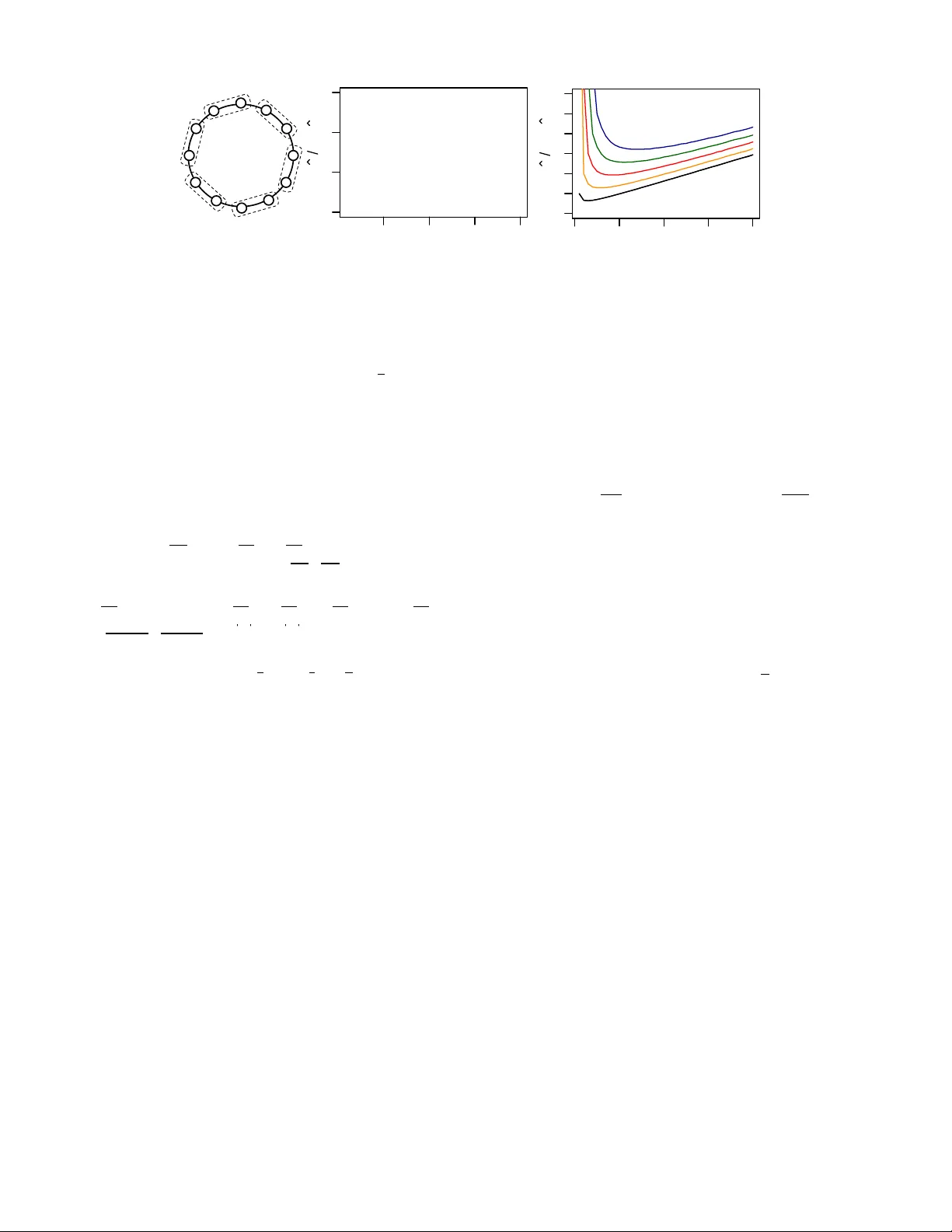
Authors: Johan Ug, er, Brian Karrer
Graph Cluster Randomization: Netw ork Exposure to Multiple Univer ses Johan Ugander Brian Karrer Lars Backstrom Jon Kleinberg Cornell University F acebook F acebook Cornell University jhu5@cor nell.edu {briankarrer ,lars}@fb .com kleinber@cs.cornell.edu ABSTRA CT A/B testing is a standard approach for ev aluating the effect of on- line experiments; the goal is to estimate the ‘a verage treatment ef- fect’ of a new feature or condition by exposing a sample of the ov erall population to it. A drawback with A/B testing is that it is poorly suited for experiments in volving social interference, when the treatment of individuals spills ov er to neighboring individuals along an underlying social network. In this work, we propose a nov el methodology using graph clustering to analyze av erage treat- ment ef fects under social interference. T o begin, we characterize graph-theoretic conditions under which indi viduals can be consid- ered to be ‘network exposed’ to an e xperiment. W e then show ho w graph cluster randomization admits an efficient exact algorithm to compute the probabilities for each vertex being network exposed under sev eral of these exposure conditions. Using these probabil- ities as in verse weights, a Horvitz-Thompson estimator can then provide an effect estimate that is unbiased, provided that the expo- sure model has been properly specified. Giv en an estimator that is unbiased, we focus on minimizing the variance. First, we dev elop simple sufficient conditions for the v ari- ance of the estimator to be asymptotically small in n , the size of the graph. Howe ver , for general randomization schemes, this v ari- ance can be lower bounded by an exponential function of the de- grees of a graph. In contrast, we show that if a graph satisfies a r estricted-gr owth condition on the growth rate of neighborhoods, then there exists a natural clustering algorithm, based on vertex neighborhoods, for which the variance of the estimator can be up- per bounded by a linear function of the degrees. Thus we show that proper cluster randomization can lead to exponentially lower esti- mator variance when experimentally measuring a verage treatment effects under interference. 1. INTR ODUCTION Social products and services – from fax machines and cell phones to online social networks – inherently exhibit ‘network effects’ with regard to their v alue to users. The value of these products to a user is inherently non-local, since it typically grows as members of the user’ s social neighborhood use the product as well. Y et random- Permission to make digital or hard copies of all or part of this work for personal or classroom use is granted without fee provided that copies are not made or distrib uted for profit or commercial adv antage and that copies bear this notice and the full citation on the first page. T o copy otherwise, to republish, to post on serv ers or to redistribute to lists, requires prior specific permission and/or a fee. Copyright 20XX A CM X-XXXXX-XX-X/XX/XX ...$15.00. ized experiments (or ‘ A/B tests’), the standard machinery of test- ing framew orks including the Rubin causal model [14], critically assume what is known as the ‘stable unit treatment value assump- tion’ (SUTV A), that each individual’ s response is affected only by their own treatment and not by the treatment of any other individ- ual. Addressing this tension between the formalism of A/B testing and the non-local effects of network interaction has emerged as a key open question in the analysis of on-line beha vior and the design of network experiments [6]. Under ordinary randomized trials where the stable unit treatment value assumption is a reasonable approximation — for example when a search engine A/B tests the effect of their color scheme upon the visitation time of their users — the population is divided into two groups: those in the ‘treatment’ group who see the new color scheme A and those in the control group who see the default color scheme B. Assuming there are negligible interference effects between users, each indi vidual in the treated group responds just as he or she would if the entire population were treated, and each in- dividual in the control group responds just as he or she would if the entire population were in control. In this manner, we can imagine that we are observing results from samples of two distinct ‘parallel univ erses’ at the same time — ‘Universe A ’ in which color scheme A is used for everyone, and ‘Universe B’ in which color scheme B is used for e veryone — and we can make inferences about the properties of user behavior in each of these uni verses. This tractable structure changes dramatically when the behavior of one user i can hav e a non-trivial effect on the behavior of another user j — as is the case when the feature or product being tested has any kind of social component. No w , if i is placed in Universe A and j is placed in Uni verse B, then our analysis of i ’ s beha vior in A is contaminated by properties of j ’ s behavior in B, and vice versa; we no longer hav e two parallel uni verses. A verage T r eatment and Network Exposure . Our goal is to de- velop techniques for analyzing the av erage effect of a treatment on a population when such interaction is present. As our basic sce- nario, we imagine testing a service by providing it to a subset of an underlying population; the service has a ‘social’ component in that i ’ s reaction to the service depends on whether a neighbor j in the social network also has the service. W e say that an individual is in the tr eatment gr oup if the individual is provided with the service for the test, and in the contr ol gr oup otherwise. There is an un- derlying numerical response variable of interest (for example, the user’ s time-on-site in each condition), and we want to estimate the av erage of this response in both the uni verse where everyone has the service, and the universe where no one has the service, despite the fact that — since the population is divided between treatment and control — we don’t ha ve direct access to either uni verse. W e express this question using a formalism introduced by Aronow and Samii for causal inference without this stable unit treatment value assumption [2], with strong similarities to similar formalism introduce by Manski [13], and adapt it to the problem of interfer- ence on social networks. Let ~ z ∈ { 0 , 1 } n be the treatment assign- ment vector , where z i = 1 means that user i is in the treatment group and z i = 0 means the user is in the control. Let Y i ( ~ z ) ∈ R be the potential outcome of user i under the treatment assignment vector ~ z . The fundamental quantity we are interested in is the av- erage treatment ef fect, τ , between the two diametrically opposite univ erses ~ z = ~ 1 and ~ z 0 = ~ 0 , τ ( ~ z = ~ 1 , ~ z 0 = ~ 0) = 1 n n X i =1 h Y i ( ~ z = ~ 1) − Y i ( ~ z 0 = ~ 0) i . (1) This formulation contains the core problem discussed in informal terms above: unlike ordinary A/B testing, no two users can ever truly be in opposing univ erses at the same time. A ke y notion that we introduce for ev aluating (1) is the notion of network exposur e . W e say that i is ‘network exposed’ to the treatment under a particular assignment ~ z 0 if i ’ s response under ~ z 0 is the same as i ’ s response in the assignment ~ 1 , where everyone receiv es the treatment. 1 W e define network exposure to the control condition analogously . W ith this definition in place, we can in vestigate sev eral possi- ble conditions that constitute network exposure. For example, one basic condition would be to say that i is network exposed to the treatment if i and all of i ’ s neighbors are treated. Another would be to fix a fraction q > 0 and say that i is network exposed if i and at least a q fraction of i ’ s neighbors are treated. The definition of network exposure is fundamentally a modeling decision by the experimenter , and in this work we introduce sev eral families of e x- posure conditions, each specifying the sets of assignment vectors in which a user is assumed to be ‘network exposed’ to the treat- ment and control universes, providing several characterizations of the continuum between the two uni verses. Choosing network ex- posure conditions is crucial because they specify when we can ob- serve the potential outcome of a user as if they were in the treatment or control univ erse, without actually placing all users into the treat- ment or control univ erse. Graph Cluster Randomization . Following the formulation of net- work exposure, a second key notion that we introduce is a generic graph randomization scheme based on graph clustering, which we call graph cluster randomization . At a high lev el, graph cluster ran- domization is a technique in which the graph is partitioned into a set of clusters , and then randomization between treatment and con- trol is performed at the cluster level. The probability that a verte x is network e xposed to treatment or control will then typically in volve a graph-theoretic question about the intersection of the set of clus- ters with the local graph structure near the vertex. W e show ho w it is possible to precisely determine the non-uniform probabilities of entering network exposure conditions under such randomization. Using in verse probability weighting [9], we are then able to derive an unbiased estimator of the a verage treatment effect τ under any network exposure for which we can explicitly compute probabili- ties. W e motiv ate the power of graph cluster randomization by fur- nishing conditions under which graph cluster randomization will produce an estimator with asymptotically small variance. First, we observe that if the graph has bounded degree and the sizes of all 1 W e also discuss adaptations to the case where the responses in these two cases dif fer only by a small parameter ε . the clusters remain bounded independent of the number of vertices n , then the estimator variance is O (1 /n ) , a simple but illustrativ e sufficient condition for smallness. The key challenge is the depen- dence on the degrees — in general, a collection of bounded-size clusters can produce a variance that grows e xponentially in the v er- tex degrees. More precisely , when performing graph cluster ran- domization with single-vertex clusters, the variance of the estima- tor admits a lower bound that depends exponentially on the degrees. This raises the important algorithmic question of how to choose the clustering: bounded-size clusters provide asymptotically small variance in the number of v ertices n , but if the clusters are not cho- sen carefully then we get an exponential dependence on the vertex degrees which could cause the v ariance to be v ery lar ge in practice. Cluster Randomization in Restricted-Growth Graphs . W e iden- tify an important class of graphs, which we call r estricted-gr owth graphs , on which a non-trivial clustering algorithm admits an up- per bound on the estimator variance that is linear in the degrees of the graph. The restricted-growth condition that we introduce for graphs is an expansion of the bounded-growth condition previ- ously introduced for studying nearest-neighbor algorithms in met- ric spaces [10], designed to include low-diameter graphs in which neighborhoods can grow exponentially . Formally , let B r ( v ) be the set of vertices within r hops of a vertex v ; our restricted-growth condition says that there e xists a constant κ , independent of the de- grees of the graph, such that for all vertices v and all r > 0 , we hav e | B r +1 ( v ) | ≤ κ | B r ( v ) | . Note the comparison to the standard bounded-growth definition, which requires | B 2 r ( v ) | ≤ κ | B r ( v ) | , a much stronger condition and not necessary for our results to hold. For restricted-growth graphs, we provide a clustering algorithm for which the estimator variance grows only linearly in the degree. The challenge is that the variance can grow exponentially with the number of clusters that intersect a verte x’ s neighborhood; our ap- proach is to form clusters from balls of fixed radius gro wn around a set of well-separated vertices. The restricted growth condition pre- vents balls from packing too closely around any one verte x, thus prev enting vertex neighborhoods from meeting too many clusters. W e note that for the special case of restricted-growth graphs that come with a uniform-density embedding in Euclidean space, one can use the locations of vertices in the embedding to carve up the space into clusters directly; the point, as in work on the nearest- neighbor problem [10], is to control this carving-up at a graph- theoretic lev el rather than a geometric one, and this is what our technique does. Our class of restricted-growth graphs provides an attractive model for certain types of real-world graphs. Restricted-gro wth graphs include graphs for which there exists an embedding of the ver - tices with approximately uniform density in a Euclidean space of bounded dimension, such as lattices or random geometric graphs, where edges connect neighbors within some maximal metric dis- tance. Summary . Our work thus occupies a mediating perch between re- cent work from the statistical literature on causal inference under interference [1, 2, 15], as well as recent work from the computer science literature on network bucket testing [3, 11]. Our contribu- tion extends upon the ordinary inference literature by developing exposure models and randomization schemes particularly suited for experiments on lar ge social graphs, also showing ho w pre vious ap- proaches are intractable. Meanwhile, we show that reducing esti- mator variance in volv es non-trivial graph-theoretic considerations, and we introduce a clustering algorithm that improves exponen- tially on baseline randomization schemes. Our contribution also connects to existing work on network bucket testing by contribut- ing an exposure framework for the full graph and a randomization scheme that is capable of considering multiple exposure conditions at once, a necessity for true concurrent causal experimentation. In Section 2 we describe our models of network exposure. In Section 3 we present our graph cluster randomization scheme, an algorithm for efficiently computing exposure probabilities, and an unbiased estimator of a verage treatment ef fects under graph cluster randomization. In Section 4 we introduce restricted-growth graphs, and sho w how the estimator has a v ariance that is linearly bounded in degree for such graphs. Section 5 concludes. 2. NETWORK EXPOSURE MODELS For A/B randomized experiments, the tr eatment condition of an individual decides whether or not they are subject to an interv en- tion. This typically takes two values: ‘treatment’ or ‘control’. In most randomized experiments, the experimenter has explicit con- trol ov er how to randomize the treatment conditions, and generally individuals are assigned independently . Meanwhile, the exposur e condition of an individual determines how they experience the in- tervention in full conjunction with how the world experiences the intervention. W ithout the stable unit treatment value assumption, at worst each of the 2 n possible values of ~ z define a distinct expo- sure condition for each user . Arono w and Samii call this “arbitrary exposure” [2], and there would be no tractable way to analyze ex- periments under arbitrary exposure. Consider the potential outcomes for user i . In the “arbitrary ex- posure" case, Y i ( ~ z ) is completely different for e very possible ~ z . This means that we will nev er be able to observe Y i ( ~ z ) for either ~ z = ~ 1 or ~ z = ~ 0 without putting all users into the treatment or control univ erses. Thus, to make progress on estimating the a ver- age treatment effect under any other conditions, we require further assumptions. W e do this here by assuming that multiple treatment vectors ~ z can map to the same potential outcomes: essentially , as long as treatment vectors ~ z and ~ z 0 are “similar enough” from the perspectiv e of a vertex i , in a sense to be made precise below , then i will ha ve the same response under ~ z and ~ z 0 . Specifically , let σ x i be the set of all assignment vectors ~ z for which i experiences outcome x . W e refer to σ x i as an exposur e condition for i ; essentially , σ x i consists of a set of assignment vec- tors that are “indistinguishble” from i ’ s point of view , in that their effects on i are the same. Our interest is in the particular exposure conditions σ 1 i and σ 0 i , which we define to be the sets that contain ~ z = ~ 1 and ~ z = ~ 0 respectively . In this way , we are assuming that for all ~ z 1 ∈ σ 1 i , we have Y i ( ~ z = ~ z 1 ) = Y i ( ~ z = ~ 1) , and for all ~ z 0 ∈ σ 0 i , we have Y i ( ~ z = ~ z 0 ) = Y i ( ~ z = ~ 0) . 2 Note that it is pos- sible that ~ z = ~ 1 and ~ z = ~ 0 belong to the same exposure condition and that σ 1 i = σ 0 i , which corresponds to a treatment that has no effects. W e define an e xposur e model for user i as a set of e xposure con- ditions that completely partition the possible assignment vectors ~ z . The set of all models, across all users, is the exposure model for an experiment. For our purposes though, it is unnecessary to entirely specify an e xposure model, since we are only trying to determine 2 If this strikes the reader as too restrictiv e a definition of “expo- sure condition”, consider instead partitioning the space of potential outcomes (rather that partitioning the space of assignment vectors) using small -sized bins, and define the “exposure conditions” as all assignment vectors that produce a potential outcome in that bin. In cases where no other potential outcomes correspond to the out- comes for ~ z = ~ 0 or ~ z = ~ 1 , it may be more appropriate to manage bias using distances on potential outcomes this way . the av erage treatment effect between the extreme universes. W e only care about the exposure conditions σ 1 i and σ 0 i for which each user i e xperiences exposure to the treatment or control uni verse 3 . Of course, the true exposure conditions σ 1 i and σ 0 i for each user are not known to the experimenter a priori, and analyzing the re- sults of an experiment requires choosing such conditions in our framew ork. If the wrong exposure conditions are chosen by the experimenter , what happens to the estimate of the av erage treat- ment ef fect? If users are responding in w ays that do not correspond to ~ z = ~ 1 and ~ z = ~ 0 , we will be introducing bias into the average treatment effect. The magnitude of this bias depends on how close the outcomes actually observed are to the outcomes at ~ z = ~ 1 and ~ z = ~ 0 that we wanted to observe. It may e ven be favorable to allow such bias in order to lower variance in the results of the e xperiment. Neighborhood Exposure . W e now describe some general expo- sure conditions that we use in what follo ws. In particular , we focus primarily on local exposur e conditions , where two assignments are indistinguishable to i if they agree in the immediate graph neigh- borhood of i . W e consider absolute and fractional conditions on the number of treated neighbors. Note we are not asserting that these possible exposure conditions are the actual exposure condi- tions with respect to the actual potential outcomes in an experiment, but rather that they provide useful abstractions for the analysis of an experiment, where again the degree of bias introduced depends on how well the e xposure conditions approximate belonging to the counterfactual uni verses. • Full neighborhood exposur e: V ertex i e xperiences full neighbor- hood exposure to a treatment condition if i and all i ’ s neighbors receiv e that treatment condition. • Absolute k -neighborhood exposur e: V ertex i of degree d , where d ≥ k , experiences absolute k -neighborhood exposure to a treat- ment condition if i and ≥ k neighbors of i recei ve that treatment condition. • F ractional q -neighborhood exposur e: V erte x i of degree d expe- riences fractional q -neighborhood exposure to a treatment condi- tion if i and ≥ qd neighbors of i receive that treatment condition. The k -absolute and q -fractional neighborhood exposures can be considered relaxations of the full neighborhood exposure for v ertex i in that they require fewer neighbors of i to have a fix ed treatment condition for i to be considered as belonging to that exposure con- dition. In fact, the set of assignment vectors that correspond to k - absolute and q -fractional neighborhood exposures are each nested under the parameters k and q respectiv ely . Increasing k or q de- creases the set of assignment vectors until reaching full neighbor- hood exposure for v ertex i . It is natural to consider heterogeneous values k or q — val- ues that differ for each user – but we limit our discussion to ex- posure conditions that are homogeneous across users as much as possible. W e do incorporate a mild heterogeneity in the definition of k -neighborhood exposure when vertices hav e degree d < k : for these vertices we consider full neighborhood exposure instead. Fractional exposure does not require this adjustment. Core Exposure . Full neighborhood exposure is clearly only an approximation of full immersion in a universe. Be yond local ex- posure conditions, we also consider e xposure condition with global dependence. As one approach, consider individuals as exposed to 3 If one was to assume functional relationships between the poten- tial outcomes in different exposure conditions then other exposure conditions besides σ 1 i and σ 0 i could become relev ant. a treatment only if they are suf ficiently surrounded by sufficiently many treated neighbors who are in turn also surrounded by suffi- ciently many treated neighbors, and so on. This recursiv e defini- tion may initially appear intractable, but such recursiv e exposure can in fact be characterized precisely by analyzing the k -core — and more generally the heterogeneous k -core — on the induced graph of treatment and control individuals. Recall that the k -core of a graph G = ( V , E ) is the maximal subgraph of G in which all vertices have degree at least k [4]. Sim- ilarly , the heterogeneous k -core of a graph G = ( V , E ) , parame- terized by a vector k = ( k 1 , . . . , k | V | ) , is the maximal subgraph H = ( V 0 , E 0 ) of G in which each vertex v i ∈ V 0 has degree at least k i [5]. Using the definition of heterogeneous k -core, we introduce the following natural fractional analog. D E FI N I T I O N 2 . 1 ( F R AC T I O NA L q - C O R E ) . The fractional q - cor e is the maximal subgraph H = ( V 0 , E 0 ) of G = ( V , E ) in which each vertex v i ∈ V 0 is connected to at least a fraction q of the vertices it was connected to in G . Thus, for all v i ∈ V 0 , deg H ( v i ) ≥ q deg G ( v i ) . Equivalently , if d i is the de gr ees of ver- tex i , the fractional q -core is the heter ogenous k -cor e of G for k = ( q d 1 , . . . , q d | V | ) . Since the heterogeneous k -core is a well-defined object, so is the fractional q -core. Using this definition, we now define expo- sure conditions that are all stricter versions of corresponding earlier neighborhood conditions. • Component exposur e: V ertex i experiences component exposure to a treatment condition if i and all of the v ertices in its connected component receiv e that treatment condition. • Absolute k -cor e exposur e: V ertex i with degree d ≥ k experi- ences absolute k -core exposure to a treatment condition if i be- longs to the k -core of the graph G [ V 0 ] , the subgraph of G in- duced on the vertices V 0 that receiv e that treatment condition. • F ractional q -core exposur e: V ertex i experiences fractional q - core exposure to a treatment condition if i belongs to the frac- tional q -core of the graph G [ V 0 ] , the subgraph of G induced on the vertices V 0 that receiv e that treatment condition. Component exposure is perhaps the strongest requirement for network exposure imaginable, and it is only feasible if the inter- ference graph being studied is comprised of many disconnected components. W e include it here specifically to note that the frac- tional q -core exposure for q = 1 reduces to component exposure. Again like the neighborhood exposure case, absolute core expo- sure requires heterogeneity in k across users for it to be a useful condition for all users. A parsimonious solution analogous to the solution for k -neighborhood exposure may be to consider heteroge- neous max(degree, k )-core exposure. Fractional q -core exposure, like fractional q -neighborhood exposure, is again free from these parsimony problems. Core exposure conditions are strictly stronger than the associated neighborhood exposure conditions abo ve. In f act, ev ery assignment vector in which a vertex i would be component or core exposed corresponds to neighborhood exposure, but not vice versa. So the assignment vectors of core and component exposure are entirely contained in those of the associated neighborhood exposure. Other Exposure Conditions . Other exposure conditions may prove relev ant to particular applications. In particular , we draw attention to the intermediate concept of placing absolute or fractional con- ditions on the population of vertices within h hops, where h = 1 is the neighborhood exposure conditions above. W e also note that on social networks with very high degree, for many applications it may be more rele vant to define the e xposure conditions in terms of a lower de gree network that considers only stronger ties. 3. RANDOMIZA TION AND ESTIMA TION Using the concept of network exposure, we can no w consider es- timating the average treatment ef fect τ between the two counterfac- tual univ erses using a randomized experiment. Recall that ~ z is the treatment assignment vector of an experiment. T o randomize the experiment, let ~ z be drawn from Z , a random v ector that takes v al- ues on { 0 , 1 } n , the range of ~ z . The distribution of Z ov er { 0 , 1 } n giv en by Pr( Z = ~ z ) is what defines our randomization scheme, and it is also exactly what determines the relev ant probabilities of network exposure. For a user i , Pr( Z ∈ σ 1 i ) is the probability of network exposure to treatment and Pr( Z ∈ σ 0 i ) is the probability of network exposure to control. In general, these probabilities will be different for each user and each treatment condition, and kno wing these probabilities makes it possible to correct for allocation bias during randomization. In par - ticular , it becomes possible to use the Horvitz-Thompson estimator, ˆ τ , to obtain an unbiased estimate of τ , here giv en by ˆ τ ( Z ) = 1 n n X i =1 Y i ( Z ) 1 [ Z ∈ σ 1 i ] Pr( Z ∈ σ 1 i ) − Y i ( Z ) 1 [ Z ∈ σ 0 i ] Pr( Z ∈ σ 0 i ) , (2) where 1 [ x ] is the indicator function. Assuming the probabilities are positiv e, the expectation o ver Z clearly gives τ , though note that this does assume that the e xposure conditions are not misspecified. Let us examine the exposure probabilities for the simplest net- work exposure condition, full neighborhood exposure, and under the simplest randomization scheme — independent v ertex random- ization, in which each vertex is independently assigned to treat- ment or control. If all v ertices are treated independently with prob- ability p ∈ (0 , 1) then the probability of full neighborhood ex- posure to treatment for a user i of degree d i is simply giv en by Pr( Z ∈ σ 1 i ) = p d i +1 , and the probability of full neighborhood exposure to control is giv en by Pr( Z ∈ σ 0 i ) = (1 − p ) d i +1 . This highlights the main challenge of network exposure: the chance that a vertex with high degree manages to reach full neighborhood ex- posure, or an ywhere near it, can be e xponentially small in d i . Intu- itiv ely , such small exposure probabilities will dramatically increase the variance of the Horvitz-Thompson estimator , and it indicates the necessity of using more intelligent randomization. T o reduce the variance of this Horvitz-Thompson estimator , we introduce a general graph cluster randomization approach, creat- ing graph clusters and randomizing assignment at the cluster lev el rather than at the v ertex level, with clusters assigned independently . Connected vertices will then be assigned to the same treatment con- dition more often than would happen with independent assignment, increasing the expected number of users who are network exposed to a condition at the cost of increased correlations between users’ exposure conditions. For clarity when discussing clustering, we introduce some nota- tion. Let the vertices be partitioned into n c clusters C 1 , . . . , C n c . Let N i ⊆ V denote the neighbors of i in the graph G , and let S i = { C j : ( i ∪ N i ) ∩ C j 6 = ∅} denote the set of clusters that contain i or a neighbor of i ; we call S i the set of clusters to which i is connected . Using this notation, we will now examine the prob- abilities of different netw ork exposures. For the general creation of clusters we defer to the literature on algorithms for graph partitioning and community detection [7, 16]. In Section 4 we describe a particular algorithm for clustering graphs that satisfy a restricted-growth condition. The remainder of this section, ho wev er , describes the behavior of an arbitrary clus- tering on an arbitrary graph. 3.1 Exposure probabilities W e now e xamine how the probabilities of network exposure can be computed given a clustering. As a simple example, for the full neighborhood exposure condition, the probability of network ex- posure to treatment simply becomes Pr( Z ∈ σ 0 i ) = p | S i | and to control becomes Pr( Z ∈ σ 1 i ) = (1 − p ) | S i | . W e now show that computing the exposure probabilities for absolute and fractional neighborhood exposure conditions is tractable as well. Consider the challenge of computing the probability that vertex i with degree d i is treated and more than k of its neighboring vertices are treated under cluster randomization. This applies when consid- ering both absolute and fractional neighborhood exposures. First, let us reindex the clusters such that if i is connected to | S i | = s clusters, i itself resides on cluster s , and we let j = 1 , . . . , s − 1 denote the other connected clusters. Let w i 1 , . . . , w is be the num- ber of connections i has to each cluster , and let the Bernoulli ( p ) random variables X 1 , . . . , X s denote the independent coin tosses associated with each cluster . Then: Pr[ Z ∈ σ 1 i ] = Pr [ X s = 1] · Pr h P s − 1 j =1 w ij X j ≥ k − w is i , Pr[ Z ∈ σ 0 i ] = Pr [ X s = 0] · Pr h P s − 1 j =1 w ij X j ≤ d i − k i . Here the random quantity P j w ij X j obeys a weighted equiv alent of a Poisson-binomial distrib ution, and the probabilities in question can be computed explicitly using a dynamic program defined by the following recursion Pr h P s j =1 w j X j ≥ T i = p Pr h P s − 1 j =1 w ij X j ≥ T − w is i + (1 − p ) Pr h P s − 1 j =1 w ij X j ≥ T i . Note that T is bounded by the maximum v ertex degree d max , mak- ing this a polynomial time dynamic program with runtime O ( d max s ) . W e formalize this computation into the follo wing proposition. P R O P O S I T I O N 3.1. The probability that vertex i is treated and ≥ k neighboring vertices ar e treated under independent cluster randomization is given by Pr[ Z ∈ σ 1 i ] = pf ( s − 1 , k − w is ; p, ~ w ) wher e f (1 , T ; p, ~ w i ) = p 1 [ T < w i 1 ] , f ( j, T ; p, ~ w i ) = pf ( j − 1 , T − w ij ; p, ~ w i ) +(1 − p ) f ( j − 1 , T ; p, ~ w i ) . The pr obability that vertex i is in contr ol and ≥ k neighboring vertices are in control under independent cluster randomization is given by Pr[ Z ∈ σ 0 i ] = (1 − p )[1 − f ( s − 1 , d i − k + 1; p, ~ w )] . Recall that these partial neighborhood exposure conditions (abso- lute and fractional) are nested. In fact, for a given verte x i the recursion can be used to derive the probability for e very possible threshold value under consideration in a single O ( d max s ) double for-loop. Such a computation in fact returns the probability distri- bution over the exposure space for each individual. See Figure 1 for illustrations of what this distribution can look lik e. The dynamic program abov e only provides a means of exactly computing exposure probabilities for absolute and fractional neigh- borhood exposure conditions. Unfortunately , ho w to efficiently Fraction of neighbors treated B 0.0 0.5 0.25 0.75 1.0 Ego A Ego B Fraction of neighbors treated B Universe A Universe B Universe B (a) (b) 0.0 0.5 0.25 0.75 1.0 Universe A Ego A Ego B Figure 1: The probability distribution over the exposure space for a single individual, where the exposure conditions σ 0 i and σ 1 i are shown in yellow for both (a) an i.i.d. vertex randomization and (b) an ideal cluster randomization, where the probability mass is collected at exposure conditions of interest. compute the exact probability of k -core and fractional q -core ex- posure conditions is unclear , but recall that these exposure condi- tions were formally nested subsets of the corresponding neighbor- hood exposure conditions. This at least allows us to upper bound the core exposure probabilities, and we formalize this connection via the follo wing proposition. Because we are generally concerned about exposure probabilities being too small, this upper bound can be useful in identifying vertices with problematically small proba- bilities already under neighborhood exposure. P R O P O S I T I O N 3.2. The pr obability vertex i is network exposed to a tr eatment condition under cor e exposur e is less than or equal to the pr obability under the analogous neighborhood exposur e: Pr( Z ∈ σ x i | k -cor e ) ≤ P r ( Z ∈ σ x i | k -nhood ) , Pr( Z ∈ σ x i | frac q -core ) ≤ P r ( Z ∈ σ x i | frac q -nhood ) . It is possible that a useful direct estimate of the core exposure probabilities can be obtained via Monte Carlo sampling of the ran- domization, but we do not e xplore that possibility here. 3.2 Estimator variance The variance of the Horvitz-Thompson estimator under inter- ference has been studied by Aronow and Samii [2], where they also present se veral variance reduction schemes. Estimating the variance under their approach requires knowledge of joint expo- sure conditions, the joint probability that vertex i is network ex- posed to treatment/control and verte x j is network exposed to treat- ment/control. This is the probability that the random vector Z is in the e xposure condition for v ertex i and for vertex j simultaneously , i.e. Pr( Z ∈ ( σ 1 i ∩ σ 1 j )) for joint network exposure to treatment. If one is interested in computing the variance of the estimator an- alytically then there is nothing fundamentally different about this probability computation when compared to the single verte x ex- posure probability , aside from the fact that the intersection of the two sets can be empty . Aronow and Samii observe that an empty intersection makes it impossible to derive an unbiased estimate of the variance (though the y show ho w the variance can still be upper bounded), but it does not bias the ef fect estimator itself. The variance of the ef fect estimator where ˆ Y x ( Z ) = 1 n X i [ Y i ( Z ) 1 [ Z ∈ σ x i ] / Pr( Z ∈ σ x i )] is giv en by V ar [ ˆ τ ( Z )] = h V ar [ ˆ Y 1 ( Z )] + V ar [ ˆ Y 0 ( Z )] − 2 Cov [ ˆ Y 1 ( Z ) , ˆ Y 0 ( Z )] i . (3) Assuming the exposure conditions are properly specified, namely assuming that Y i ( ~ z ) is constant for all ~ z ∈ σ x i , we can introduce the notation Y i ( σ x i ) := Y i ( ~ z ∈ σ x i ) . Using the further notation π x i := P r [ Z ∈ σ x i ] and π xy ij := P r [ Z ∈ ( x i ∪ σ y j )] we obtain V ar [ ˆ Y x ( Z )] = 1 n 2 " n X i =1 1 − π x i π x i Y i ( σ x i ) 2 + n X i =1 n X j =1 j 6 = i π xx ij − π x i π x j π x i π x j Y i ( σ x i ) Y j ( σ x j ) # , (4) and Cov [ ˆ Y 1 ( Z ) , ˆ Y 0 ( Z )] = 1 n 2 " n X i =1 n X j =1 j 6 = i π 10 ij − π 1 i π 0 j π 1 i π 0 j Y i ( σ 1 i ) Y j ( σ 0 j ) − n X i =1 Y i ( σ 1 i ) Y i ( 0 i ) # . (5) The abov e expressions make it evident that the variance is v ery tightly controlled by the probabilities of exposure, and in order to upper bound the variance we will require lower bounds on the prob- abilities π x i and also upper bounds on the joint probabilities π xy ij , for all vertex pairs and all combinations of x and y . For neighbor- hood exposure, we can now write basic sufficient conditions under which the variance of the estimator is asymptotically O (1 /n ) in n for graph cluster randomization. P R O P O S I T I O N 3.3. Assume the potential outcomes Y i ( · ) are all O (1) in n . If G has maximum de gree O (1) and the size of each cluster is O (1) , then the variance of the Horvitz-Thompson estima- tor for full, k -neighborhood, and q -fractional neighborhood expo- sur e under graph cluster randomization is O (1 /n ) . P R O O F . Assume G has maximum degree O (1) and the size of each cluster is O (1) . All of the single sums are clearly O ( n ) : π x i is O (1) since all vertices ha ve bounded degree. For the double sums, note that π xx ij = π x i π x j if and only if i and j hav e no common clus- ter neighbors, | S i ∩ S j | = 0 . Whenever | S i ∩ S j | > 0 , π xx ij > π x i π x j for full, k -neighborhood, and q -fractional neighborhood exposure. Further , π 10 ij < π 1 i π 0 j if | S i ∩ S j | > 0 and π 10 ij = π 1 i π 0 j otherwise. So the terms of the double sums are zero whenever π ij = π i π j and when the terms are not zero ( | S i ∩ S j | > 0 ), they are all positive and bounded above O (1) due to the bounded degrees. W e now bound the number of vertices j for which | S i ∩ S j | > 0 . V erte x i at most connects to O (1) clusters and therefore | S i | = O (1) . For all C ∈ S i , we have that | S i ∩ S j | > 0 for any j ∈ C and for any verte x j that is adjacent to a vertex in cluster C . Both of these contributions is O (1) , giving an O (1) contrib ution of vertices for each C ∈ S i . Since there are O (1) such clusters, this is still O (1) vertices j in total for v ertex i such that | S i ∩ S j | > 0 . Thus for each verte x, at most O (1) of the terms in the double sum are positive, making the total variance O (1 /n ) . The strength of this general result is that it achiev es an O (1 /n ) bound on the variance when the maximum de gree is bounded. The problem is that the variance can grow exponentially in the degrees of the graph. In this next section we address this issue, introducing a condition on a graph that ensures we can find a clustering into sets of size O (1) — consistent with the above result – for which the variance grows as O (1 /n ) but is also linear rather than e xponential in the maximum degree. 4. V ARIANCE ON RESTRICTED-GR O WTH GRAPHS In order to measure average treatment effects under interference on large-scale graphs, it is necessary to design a randomization scheme capable of containing the estimator variance for high-degree vertices. In this section we show that any graph satisfying our restricted-growth condition admits a clustering that can produce an unbiased ef fect estimate that is both O (1 /n ) and linear in the degrees of the graph. In contrast, we show that with less careful clustering, it is easy for the variance to gro w exponentially in the degrees. Let us first define restricted-growth graphs. Let B r ( v ) be the set of vertices within r hops of a vertex v . D E FI N I T I O N 4.1. A graph G = ( V , E ) is a r estricted-gr owth graph if for all vertices v ∈ V and all r > 0 , we have | B r +1 ( v ) | ≤ κ | B r ( v ) | . As mentioned in the introduction, graphs derived from a uniform- density embedding in a Euclidean space of dimension m exhibit restricted growth, with growth constant κ = 2 m independent of degree. T o develop intuition for the restricted-growth assumption, we first analyze the variance using graph cluster randomization on a family of particularly tractable restricted-growth graphs, k th pow- ers of the cycle. W e follow this analysis by proving bounds on the variance for general restricted-gro wth graphs. 4.1 Cycle and powers of the cycle examples First we will consider a simple graph consisting of a single cy- cle with n vertices. F or this graph, we consider the full neigh- borhood exposure model, where we are interested in the average treatment effect between σ 1 i , when a vertex is treated and both of their neighbors are treated, and σ 0 i , when a v ertex is not treated and neither of their neighbors are treated. For the fixed responses of the vertices to treatment and control, we assume that all vertices uniformly respond Y i ( σ 1 i ) = ¯ Y to network exposure to the treat- ment and Y i ( σ 0 i ) = 0 to network exposure to the control. The cycle graph clearly admits an intuitively obvious clustering using the cycle structure, with contiguous blocks of c vertices random- ized together . As a last assumption, assume that clusters are se- lected under a balanced randomization with p = 1 / 2 . Our goal is to determine ho w the variance of the Horvitz-Thompson average treatment effect estimator depends on the size c of these clusters. For this basic combination of graph, e xposure condition, responses, and clustering, one can deriv e the asymptotic variance e xactly . Consider the variance presented in (3) above. Since all vertices respond zero to the control condition in our example, as long as the exposure probability for the control condition is strictly positive then both V ar ( ˆ Y ( σ 0 )) and Co v ( ˆ Y ( σ 1 ) , ˆ Y ( σ 0 )) are zero. Since our calculations will rely only on probabilities π 1 i for the exposure to treatment condition, we omit the superscript. The variance is then: V ar [ ˆ τ ( Z )] = ¯ Y 2 n 2 " n X i =1 1 π i − 1 + n X i =1 n X j =1 j 6 = i π ij π i π j − 1 # . (6) Notice that the terms of the double sum are only non-zero for v ertex pairs where π ij 6 = π i π j . First, consider the case of each vertex being its own cluster. The probability of being exposed and both of one’ s neighbors be- ing exposed is equal to the probability of seeing three independent coins come up heads. When the randomization is balanced (e.g. p = 1 / 2 ), we obtain π i = 1 / 8 , ∀ i . Note that the co-assignment probabilities depend on whether vertices i and j are neighbors or (a) (b) (c) ● ● ● ● ● ● ● ● ● ● ● ● ● ● ● ● ● ● ● ● ● ● ● ● ● ● ● ● ● ● ● ● ● ● ● ● ● ● ● ● 0 10 20 30 40 0 1 2 3 4 5 6 vertices per cluster, c Var kc ( τ ) Var 11 ( τ ) ● ● ● ● ● ● ● ● ● ● ● ● ● ● ● ● ● ● ● ● ● ● ● ● ● ● ● ● ● ● ● ● ● ● ● ● ● ● ● ● ● ● ● ● ● ● ● ● ● ● ● ● ● ● ● ● ● ● ● ● ● ● ● ● ● ● ● ● ● ● ● ● ● ● ● ● ● ● ● ● ● ● ● ● ● ● ● ● ● ● ● ● ● ● ● ● ● ● ● ● ● ● ● ● ● ● ● ● ● ● ● ● ● ● ● ● ● ● ● ● ● ● ● ● ● ● ● ● ● ● ● ● ● ● ● ● ● ● ● ● ● ● ● ● ● ● ● ● ● ● ● ● ● ● ● ● ● ● ● ● ● ● ● ● ● ● ● ● ● ● ● ● ● ● ● ● ● ● ● ● ● ● ● ● ● ● ● ● ● ● ● ● ● ● ● ● k=1 k=2 k=3 k=4 k=5 ● ● ● ● ● ● ● ● ● ● ● ● ● ● ● ● ● ● ● ● 5 10 15 20 0.5 1.0 1.5 2.0 vertices per cluster, c Var c ( τ ) Var 1 ( τ ) Figure 2: The cycle graph, (a) where vertices respond ¯ Y to treatment and 0 to control, shown clustered in groups of c = 2 vertices. (b) Asymptotic variance of the estimator for this graph as a function of the number of vertices per cluster , normalized by estimator variance for c = 1 vertices per cluster . (c) Simulated variance of the estimator for k th powers of the cycle graph for k = 1 , . . . , 5 as a function of the number of vertices per cluster . For each k the variance for cluster size c = 2 k + 1 gr ows linearly in k . share a neighbor . From this we derive π ij = 1 / 16 if | i − j | = 1 and π ij = 1 / 32 if | i − j | = 2 , and if | i − j | > 2 , the probabilities are independent. W e obtain V ar ( ˆ τ ( Z )) = (15 / 2) ¯ Y 2 1 n + O (1 /n 2 ) . Now , consider randomizing blocks of c ≥ 2 vertices, where c does not depend on n . The calculations for this case are expansiv e but straight-forward. W e consider a single one of the equiv alent cyclically shifted possibilities. The calculation requires handling c = 2 and c ≥ 3 separately , but the expression for c ≥ 3 as a function of c holds for c = 2 as well, so we omit the special case for brevity . The variance calculation depends on distance ∆ = | i − j | up to ∆ = c + 1 , and for c ≥ 3 this e valuates to: V ar [ ˆ τ ( Z )] = ¯ Y 2 n 2 " n + 4 n c + 2 n c ( c + 2) | {z } ∆=1 + 2 n c c − 2 X k =2 ( c − k + 2) | {z } 1 < ∆ 0 , we have | B r +1 ( v ) | ≤ κ | B r ( v ) | . Importantly , r = 0 is different: B 0 ( v ) is the singleton set { v } , while B 1 ( v ) is the neighborhood of v and hence has size d + 1 . Thus | B 1 ( v ) | / | B 0 ( v ) | = d + 1 , potentially much larger than the bound of κ on the ratio | B r +1 ( v ) | / | B r ( v ) | for r > 0 . This is the crux of the restricted-gro wth condition: from radius 0 to 1 we ha ve unrestricted growth (a factor of d + 1 ), but then the growth slows to factors of κ which can be bounded separately from d . In the language of metric spaces, we will cluster the graph using a 3-net for the shortest-path metric of G [8]. Formally , in a metric space X , an r -net Y ⊆ X is a collection of points that are mutu- ally at distance at least r from each other, but the union of all their r -balls covers the space, X ⊆ ∪ y ∈ Y B r ( y ) . Accordingly , we call our construction a 3-net clustering of the graph. T o build a 3-net clustering, we will iterativ ely identify vertices v 1 , v 2 , ... , ‘mark- ing’ vertices as we do this. Afterwards we will identify clusters C 1 , C 2 , ... to go with these vertices. More explicitly , we perform the following procedure consisting of tw o principle stages: • Initially all vertices are unmarked. • While there are unmarked vertices, in step j find an arbitrary unmarked vertex v , selecting v to be vertex v j and marking all vertices in B 2 ( v j ) . • Suppose k such vertices are defined, and let S = { v 1 , v 2 , ..., v k } . • For ev ery vertex w of G , assign w to the closest vertex v i ∈ S , breaking ties consistently (e.g. in order of lowest index). • For e very v j , let C j be the set of all vertices assigned to v j . The sets C 1 , . . . , C k are then our 3-net clustering. The k ey prop- erty of this clustering is the following result, which establishes that each vertex is connected to a number of clusters that can be bounded by a function of κ , independent of the degree. P R O P O S I T I O N 4.2. Consider any 3-net clustering of a graph G = ( V , E ) . F or all w ∈ V , the neighborhood B 1 ( w ) has a non-empty intersection with at most κ 3 distinct clusters. P R O O F . W e first claim that for all v j ∈ S , we hav e C j ⊆ B 2 ( v j ) . Indeed, consider any vertex w 6 = v j in C j . W e have w 6∈ S , since otherwise w would belong to the cluster identified with itself. Now , consider the iteration i in which w was marked; we have w ∈ B 2 ( v i ) . Since w ∈ C j and it is assigned to the closest verte x in S , it follo ws that w ∈ B 2 ( v j ) . Thus C j ⊆ B 2 ( v j ) . Next, we claim that for all v i , v j ∈ S , the sets B 1 ( v i ) and B 1 ( v j ) are disjoint. Suppose by way of contradiction that B 1 ( v i ) ∩ B 1 ( v j ) 6 = ∅ . It would follow that v i ∈ B 2 ( v j ) and vice versa. But then if we consider the vertex among v i and v j that was added to S first, the other of v i or v j would hav e been marked in that iter- ation, and hence it could not have been added to S as well. This contradiction establishes that B 1 ( v i ) and B 1 ( v j ) are disjoint. T o complete the proof, suppose by way of contradiction that B 1 ( w ) has a non-empty intersection with more than κ 3 distinct clusters: for some t > κ 3 , let u 1 , u 2 , . . . , u t be distinct vertices in B 1 ( w ) and v i 1 , . . . , v i t be distinct vertices in S such that u h ∈ C i h for h = 1 , 2 , . . . , t . Since C i h ⊆ B 2 ( v i h ) , and C i h contains a vertex adjacent to w (or contains w itself), we hav e v i h ∈ B 3 ( w ) , and hence B 1 ( v i h ) ⊆ B 4 ( w ) . The neighborhoods B 1 ( v i 1 ) , B 1 ( v i 2 ) , . . . , B 1 ( v i t ) are all pairwise disjoint as argued above, and they are all contained in B 4 ( w ) , which implies that | B 4 ( w ) | ≥ t ( d + 1) > κ 3 ( d + 1) . But applying the bounded growth inequality | B r +1 ( w ) | ≤ κ | B r ( w ) | three times we have | B 4 ( w ) | ≤ κ 3 ( d + 1) , a contradiction. This establishes that B 1 ( w ) can have a non-empty intersection with at most κ 3 distinct clusters. The above result is formulated for d -regular graphs. But in fact one can show a weaker bound depending only on κ as in Propo- sition 4.2 even for arbitrary restricted-growth graphs, without any requirement on the degrees. This weaker bound of κ 6 can be es- tablished by observing that any restricted-growth graph exhibits a “bounded gradient” on the vertex degrees, whereby vertices that are near each other in the graph must ha ve similar degrees. Combining this fact with proof of Proposition 4.2 leads to the desired bound. 4.3 V ariance bounds W e now apply the above results to bound the v ariance of the effect estimator ˆ τ . Throughout this section we assume that all responses obey upper bounds and positiv e lower bounds, Y x i ∈ [ Y m , Y M ] for both exposure to treatment and control, x = 0 , 1 . The reason for the positive lower bounds is that without them the users could all be responding zero to all treatments, making the variance zero regardless of the treatment scheme. W e also assume the ran- domization probability p is not degenerate, i.e. p ∈ (0 , 1) . W e present the results for d -regular graphs to keep expressions man- ageable, but analogous results can be deri ved for arbitrary de grees. W e first establish an exponential lower bound for the variance under vertex-le vel randomization, and then we show a contrasting linear upper bound for the v ariance under our 3-net cluster random- ization scheme. P R O P O S I T I O N 4.3. The variance of the HT estimator under full neighborhood exposur e for vertex randomization of a graph with n vertices is lower bounded by an exponential function in the de gr ee d of the graph, V ar [ ˆ τ ( Z )] ≥ O (1 /n )( p − ( d +1) +(1 − p ) − ( d +1) − 1) . P R O O F . The joint assignment probabilities for two v ertices ha v- ing the same exposure is at least the product of their individual probabilities, π xx ij ≥ π x i π x j for x = 0 , 1 . Thus the double sum in equation (4) is non-neg ativ e. Similarly , for opposing exposure con- ditions, we have π xy ij ≤ π x i π y j for x 6 = y , which makes equation (5) a non-negativ e contrib ution to equation (3). W e focus our lower bound on the main term of equation (4). Inputting the probabilities π 1 i = p d +1 and π 0 i = (1 − p ) d +1 and lower bounding responses giv es us the desired result. V ar [ ˆ τ ( Z )] ≥ 1 n 2 " n X i =1 ( 1 π 1 i − 1)( Y 1 i ) 2 + n X i =1 ( 1 π 0 i − 1)( Y 0 i ) 2 # ≥ Y 2 m n ( p − ( d +1) + (1 − p ) − ( d +1) − 2) . 2 For graphs with arbitrary degree distributions, this bound be- comes V ar [ ˆ τ ( Z )] ≥ O (1 /n ) P n i =1 ( p − ( d i +1) + (1 − p ) − ( d i +1) − 2) , which is exponential in the degree of each v ertex, meaning that ev en a single high degree v ertices can easily explode the v ariance. W e now turn to our linear upper bound for growth-restricted graphs when using our 3-net clustering. P R O P O S I T I O N 4.4. The variance of the HT estimator under full, q -fractional, or k -absolute neighborhood exposur e for a 3-net clus- ter randomization of a r estricted-gr owth graph is upper bounded by a function linear in the de gr ee d of the graph. P R O O F . Recall that the variance of the estimator is given by: V ar ( ˆ τ ( Z )) = V ar ( ˆ Y 1 ) + V ar ( ˆ Y 0 ) − 2 Cov ( ˆ Y 1 , ˆ Y 0 ) . W e begin by upper bounding the variance of ˆ Y 1 ( Z ) , and the upper bound for ˆ Y 0 ( Z ) follows the same principle. W e conclude by bounding the cov ariance term. By Proposition 4.2, each vertex is connected to at most κ 3 clusters. Thus we have the lower bound π 1 i ≥ p κ 3 , for both full and fractional neighborhood exposure. V ar [ ˆ Y 1 ( Z )] ≤ Y 2 M n 2 " n ( 1 p κ 3 − 1) + n X i =1 n X j =1 j 6 = i ( π 1 ij π 1 i π 1 j − 1) # . For each vertex i , the inner of the two sums is only nonzero at those vertices j for which the assignments are dependent. If the assignments for i and j are dependent, then they must each have neighbors in the same cluster C h associated with a vertex v h in the set of cluster centers. Since the proof of Proposition 4.2 established that C h ⊆ B 2 ( v h ) , it follows that i and j are each within distance 3 of v h and hence within distance 6 of each other . Thus, any j whose assignment is dependent on i ’ s must lie within B 6 ( i ) , and so by the restricted-growth condition, there can be at most | B 6 ( i ) | ≤ κ 5 | B 1 ( i ) | = κ 5 ( d + 1) such vertices j . Thus the sum over such j has at most κ 5 ( d + 1) terms. Also, π 1 ij ≤ p applies, since the two vertices must depend on at least one cluster . W e obtain V ar [ ˆ Y 1 ( Z )] ≤ Y 2 M [( p − κ 3 − 1) + κ 5 ( d + 1)( p − 2 κ 3 − 1 − 1)] 1 n . Now , consider the contribution of the covariance term to the vari- ance, − 2 Cov ( ˆ Y 1 , ˆ Y 0 ) , a positive quantity . Starting from equation (5), we apply the upper bound for the responses Y i to obtain − 2 Cov [ ˆ Y 1 ( Z ) , ˆ Y 0 ( Z )] ≤ − 2 Y 2 M n 2 n X i =1 n X j =1 j 6 = i π 10 ij π 1 i π 0 j − 1 + 2 Y 2 M n . As with the pre vious analogous e xpression, for each i the inner sum is non-zero for at most κ 5 ( d + 1) other vertices j . For the remaining terms, the quantity − ( π 10 ij / ( π 1 i π 0 j ) − 1) is trivially upper bounded by 1 . Thus we obtain − 2 Cov [ ˆ Y 1 ( Z ) , ˆ Y 0 ( Z )] ≤ 2 Y 2 M n [ κ 5 ( d + 1) + 1] . Combining the upper bounds, we obtain a total upper bound that is linear in degree, as desired. The restricted-growth condition we used was deri ved for regular graphs, but as we noted earlier, for restricted-gro wth graphs with arbitrary degree distributions we can apply a weaker but still con- stant bound on the cluster dependencies to obtain a variance bound that is still linear in the degree. 5. CONCLUSION The design of online experiments is a topic with many open di- rections (see e.g. [12]); in this work we have focused on the open question of A/B testing when treatment effects can spill over along the links of an underlying social network. W e introduced a basic framew ork for reasoning about this issue, as well as an algorith- mic approach — graph cluster randomization — for designing A/B randomizations of a population when network spillover effects are anticipated. Appropriate clustering can lead to reductions in vari- ance that are exponential in the vertex degrees. W e emphasize that beyond the class of graphs where we prov e bounds, graph clus- ter randomization is a technique that can be applied to arbitrary graphs using arbitrary community detection or graph partitioning algorithms, though we do not provide any variance bound guaran- tees for these scenarios. There are many further directions for research suggested by the framew ork dev eloped here. A first direction is to formulate a com- putationally tractable objectiv e function for minimizing the v ari- ance of the Horvitz-Thompson estimator . One approach would be via minimizing an adversarial variance, as in [11]. Another prob- lem that may be relev ant is to find a clustering that minimizes A/A variance for full neighborhood exposure under the assumption of known control potential outcomes. Can good clusterings for A/A variance lead to good solutions for A/B testing? W e note that A/A variance minimization would not be useful when the treatment is expected to be dominated by heterogeneous responses. Adding further structure to the potential treatment responses is another interesting direction. W e currently hav e a discrete notion of network exposure to treatment and control, b ut one could ask about responses that depend continuously on the extent of exposure. As one simple example, we could consider a response that was lin- ear in k , when a verte x had k exposed neighbors. How could we properly take advantage of such structure to get better estimates? Methods for analyzing bias under network exposure condition mis- specification would also be a natural addition to the frame work. 6. REFERENCES [1] E. Airoldi, E. Kao, P . T oulis, D. Rubin. Causal estimation of peer influence effects. In ICML , 2013. [2] P . Aronow and C. Samii. Estimating av erage causal effects under general interference. W orking P aper , September 2012. [3] L. Backstrom and J. Kleinberg. Network b ucket testing. In WWW , 2011. [4] B. Bollobás. Random graphs . Cambridge Univ . Press, 2001. [5] D. Cellai, A. Lawlor , K. Dawson, J. Gleeson. Critical phenomena in heterogeneous k-core percolation. Phys Rev E , 87(2):022134, 2013. [6] S. Fienberg. A brief history of statistical models for network analysis and open challenges. J. Comp. Graph. Stat. , 2012. [7] S. Fortunato. Community detection in graphs. Physics Reports , 486(3):75–174, 2010. [8] A. Gupta, R. Krauthgamer , J. Lee. Bounded geometries, fractals, and low-distortion embeddings. In FOCS , 2003. [9] D. Horvitz, D. Thompson. A generalization of sampling without replacement from a finite univ erse. J ASA , 1952 [10] D. Karger , M. Ruhl. Finding nearest neighbors in growth-restricted metrics. In STOC , 2002. [11] L. Katzir , E. Liberty , O. Somekh. Framework and algorithms for network buck et testing. In WWW , 2012. [12] R. Koha vi, A. Deng, B. Frasca, R. Longbotham, T . W alker , Y . Xu. T rustworthy online controlled experiments: five puzzling outcomes explained. In KDD , 2012. [13] C. Manski. Identification of treatment response with social interactions. The Econometrics Journal , 16(1):S1–S23, 2013. [14] D. Rubin. Estimating causal effects of treatments in randomized and nonrandomized studies. J. Ed. Psych. , 1974. [15] E. Tchetgen, T . V anderW eele. On causal inference in the presence of interference. Stat. Meth. Med. Res. , 2012. [16] J. Ugander , L. Backstrom. Balanced label propagation for partitioning massiv e graphs. In WSDM , 2013. [17] D. J. W atts and S. H. Strogatz. Collectiv e dynamics of ‘small-world’ networks. Natur e , 393(6684):440–442, 1998.
Original Paper
Loading high-quality paper...
Comments & Academic Discussion
Loading comments...
Leave a Comment