Reinforcement Learning for the Soccer Dribbling Task

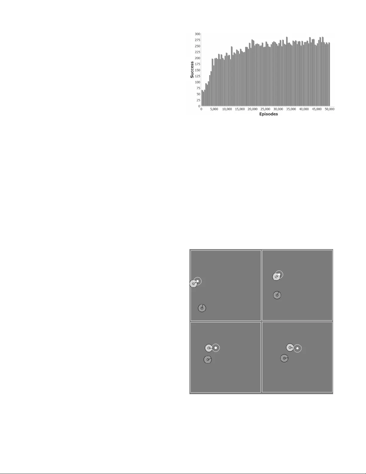
Reinf or c ement Learnin g f or the Socc er Drib bling T ask Arthur Carvalho and Renato Oli veira Abstract —W e propose a reinf orcement learning solution to the so ccer dribbling task , a scenario in which a soccer agent has to go from the beginning to the end of a region keeping possession of the ball, as an adversary attempts to gain possession. While the adversary uses a stationary policy , the dribbler lea rns the best action t o take at each decision point . After d efining meaningful variables to represent the state sp ace, and high-l ev el macro -actions to i ncorporate domain k nowledge, we d escribe our application of the reinfor cement learning algorithm Sarsa with CMA C for function app roxima ti on. Our experiments show that, after the training period, the dribbler i s able to accom p lish its task against a strong adversary around 58% of the time. I . I N T R O D U C T I O N Soccer dribblin g con sists o f th e ability of a soccer agent to go f rom th e beginning to the end of a region keeping possession o f the ball, while an adversary attempts to gain possession. In this work, we focus on the dribbler ’ s learn ing process, i.e. , the learn ing of a n effecti ve p olicy that determ ines a goo d action for the drib bler to take at each decision point. W e study the soccer dribbling task using the RoboCup soccer simulator [1]. Sp ecific details of this simulato r inc rease the complexity of the learning process. For example, besides the ad versarial and real-time environment, agents’ pe rceptions and actions are noisy and asynch ronou s. W e mod el the soccer dribbling task as a r einforcement learning pr oblem. Our solution to this pro blem combines the Sarsa algorithm with CMA C fo r f unction approxima tion. Despite the fact that the resulting learn ing algorithm is n ot guaran teed to conver g e to the optimal policy in all cases, m any lines of e v idence su ggest that it conv erges to near-optimal policies (for examp le, see [2], [3], [4], [ 5]). Besides this intr oductor y section, the r est of this pap er is organized as follows. In the next section, we d escribe the soccer dribbling task. In Section 3, we show how to map this task on to an episodic r einforcem ent learn ing framework. In Section 4 and 5, we present, respectively , the reinf orcement learning algo rithm and its re sults again st a strong adversary . In Section 6, we review the literature r elated to our work. In Section 7 , we conclu de and present futu re research directio ns. I I . S O C C E R D R I B B L I N G Soccer dribbling is a crucial skill for an ag ent to beco me a successful soccer play er . It co nsists of the ability of a soccer ag ent, hence forth called th e dribbler , to go from the beginning to the end of a region keeping possession of the ball, while an adversary attemp ts to gain possession. W e can see soccer dribbling as a subpr oblem of the co mplete soccer domain. Th e main sim plification is that th e play ers inv olved are o nly fo cused on sp ecific g oals, witho ut worrying a bout team strategies or unr elated individual skills ( e.g. , passing an d shooting) . Nevertheless, a successful po licy learn ed by th e dribbler can b e used in the complete soccer do main wh enever a soccer ag ent faces a dribbling situation . Since our focus is on the dr ibbler’ s learn ing pro cess, an omniscient coach a gent is used to man age the play . At the beginning of ea ch trial ( episode ), th e coach resets the lo cation of the b all an d o f the play ers within a training field . The dribbler is placed in th e center-left region tog ether with the ball. The adversary is placed in a rando m p osition with the constraint tha t it does not start with p ossession of the ball. An example of a starting con figuration is shown in Figure 1. Whenever the adversary gains po ssession for a set period of time o r w hen the b all goes out of the train ing field by crossing either the left line or th e top line o r the bottom line, the coach declar es the adversary as the winn er o f the episode. If the ball go es out of the tr aining field b y cro ssing the right line, then the winner is the first player to intercept the ball. After d eclaring the winner of an episode, the coach resets the location of the player s and o f the b all within the train ing field and starts a new episode. Thus, the dribb ler’ s g oal is to reach the right line tha t delimits th e training field with the ball. W e call this task the soccer dribbling task . W e argu e that th e soccer dribbling task is an excellen t benchm ark for compar ing different machine learnin g tech- niques since it in volves a comp lex proble m, and it has a well-defined objective, which is to maxim ize the numbe r o f episodes won by the drib bler . W e study the soccer d ribbling task using th e RoboCup soccer simu lator [1]. The Rob oCup socce r simulator operates in discrete time steps, each representing 1 00 milliseconds of simulated tim e. Specific details of this simulator incre ase the complexity of the learning process. For example, rand om noise is injec ted into all perc eptions and action s. Furthe r , agents m ust sense and act asynchro nously . Each soccer ag ent re ceiv es v isual inform ation about o ther ob jects every 150 millisecon ds, e.g. , its d istance Fig. 1. Example of a starting configuration. from oth er players in its curren t field of view . Eac h agent has also a bod y sensor, which detects its cu rrent “physical status” e very 100 milliseconds, e.g. , that agen t’ s stamina and spee d. Agents may execute a param eterized primitive action every 100 milliseco nds, e.g. , turn (an gle), d ash (power), and kick (power , an gle). Full details of the RoboCup socc er simulator are pr esented by Chen et al. [6]. Since p ossession is not well- defined in the RoboCup soccer simulator, we con sider th at a n age nt has possession o f the b all whenever the ball is close enoug h to be kicked, i.e. , it is in a distance less th an 1 . 085 meters fro m the agent. I I I . T H E S O C C E R D R I B B L I N G T A S K A S A R E I N F O R C E M E N T L E A R N I N G P RO B L E M In the soccer dribbling task, an ep isode begins wh en the dribbler m ay take the first action . When an episode ends ( e.g. , when the adversary g ains po ssession f or a set p eriod of time) , th e coach starts a new one, th ereby giving rise to a series o f ep isodes. Th us, the interaction b etween the dribble r and th e e n vir onment naturally breaks d own into a sequence of distinc t ep isodes. This po int, together with the fact that the Rob oCup soccer simulator oper ates in discrete time steps, allows the so ccer d ribbling task to be map ped onto a discrete- time, episodic rein forcemen t-learning fram ew or k. Roughly speaking , reinforcement learning is con cerned with how an age nt must take a ctions in an environment so as to maximize the expected lo ng-term re ward [ 7]. Like in a trial- and-err or search, the learner mu st discover wh ich actio n is the most rew ard ing one in a gi ven state of the w o rld. Thus, solving a reinfo rcement learnin g problem means finding a f unction ( policy ) tha t maps states to actio ns so th at it max imizes a re ward over the long run . As a way of incorpor ating domain knowledge, the action s available to the dr ibbler are the following h igh-level macr o -actions , wh ich are built o n the simulator’ s primitive actio ns 1 : • HoldBall ( ): The dribbler holds th e ball c lose to its bo dy , keeping it in a po sition that is difficult fo r the adversary to gain possession; • Dribble ( Θ , k ): The drib bler tu rns its b ody tow ar ds th e global angle Θ , kicks the ball k m eters ahead of it, and moves to intercept the ball. The global angle Θ is in the range [0 , 360] . In detail, th e center of the tr aining field h as been ch osen as th e orig in o f the system, wh ere the zero-an gle p oints towards th e midd le of th e right line that delimits the training field, and it increases in the clockwise direction . Tho se macro-actions are based on high- lev el skills used b y the UvA Trilearn 2003 tea m [8]. The first one maps directly onto the primitiv e action kick . Consequently , it usually takes a single time step to be p erform ed. The seco nd one, howev e r , requires an extended sequen ce of the primitive actions tu rn , kick , an d da sh . T o handle th is situatio n, we treat the so ccer d ribbling task as a semi-Markov decision p r ocess (SMDP) [9]. 1 Hencefort h, we use the terms actio n and macr o-action inte rchangeably , while alw ays distinguishing primitive actions . Formally , an SMDP is a 5 -tuple < S, A, P, r, F > , wh ere S is a countable set of states, A is a countable set of actions, P ( s ′ | s, a ) , fo r s ′ , s ∈ S , and a ∈ A , is a p robability distribu- tion provid ing the transition model between states, r ( s, a ) ∈ ℜ is a r ew ard associated with the transition ( s, a ) , an d F ( τ | s , a ) is a prob ability distribution indicating the sojourn time in a giv en state s ∈ S , i.e. , th e tim e before tr ansition provided that action a was taken in state s . Let a i ∈ A b e the i th macro- action selected by the dribbler . Thus, several simulator ’ s time steps may elapse b etween a i and a i +1 . Let s i +1 ∈ S and r i +1 ∈ ℜ be, respe cti vely , th e state and the reward following the macro-a ction a i . From the dribbler ’ s p oint o f view , an episode consists of a sequence of SMDP steps, i. e. , a sequen ce of states, macr o-actions, and rew ar ds: s 0 , a 0 , r 1 , s 1 , . . . , s i , a i , r i +1 , s i +1 , . . . , a n − 1 , r n , s n , where a i is chosen based exclusiv ely on the state s i , and s n is a terminal state in wh ich eith er the adversary or the drib bler is declared the winn er o f the episode by the coach. In th e former case, the dribbler receives the reward r n = − 1 , while in the latter case its rew a rd is r n = 1 . The intermed iate rewards are always equ al to zero, i.e. , r 1 = r 2 = · · · = r n − 1 = 0 . Thus, our objective is to find a policy th at maximizes the dribbler’ s rew ar d, i.e. , the number o f ep isodes in which it is the winner . A. Dribbler The dribb ler m ust take a decision at each SMDP step by selecting an a vailable mac ro-action. Besides th e m acro-action HoldBall , the set of actions av ailab le to th e dribb ler contains four instances of the ma cro-action Dribble : Dribble ( 3 0 ◦ , 5 ), Dribble ( 330 ◦ , 5 ), D ribble ( 0 ◦ , 5 ), and Dribble ( 0 ◦ , 10 ). Th us, besides hiding the b all fr om th e ad versary , the dribbler can kick th e b all f orward (stro ngly and weak ly), diago nally up- ward, and d iagonally downward. If at some time step the dribbler has not possession o f the ba ll and the current state is not a termina l state, then it usually means that the dribble r chose a n instance of the macro -action Dribble befo re and it is currently moving to interce pt the ball. W e turn now to the state representatio n used by th e dr ibbler . It c onsists of a set of state variables which are based on informa tion re lated to th e b all, the adversary , and the dribb ler itself. Let ang ( x ) be the glo bal angle of the object x , and ang ( x, y ) and dist ( x, y ) be, respectively , the relativ e angle and the distance between the objects x and y . Further, let w and h be , respectively , the width and the h eight of the training field. Finally , let posY ( x ) be a fu nction indicatin g whether the object x is close to ( less than 1 meter away f rom) the top line or the bottom line that delimits the tr aining field. In the for mer case, posY ( x ) = 1 , whereas in th e latter case posY ( x ) = − 1 , and oth erwise posY ( x ) = 0 . T ab le 1 shows the state variables together with th eir ranges. The first thr ee variables help the dribbler to locate itself and the adversary inside the training field. T ogeth er , the last two variables can be seen as a point d escribing th e po sition of the adversary in a polar coord inate system, wh ere the ball is the pole. Thu s, these v ar iables are used by the dr ibbler to locate th e adversary with respect to the ball. It is in teresting to T ABLE I D E S C R I P T I O N O F T H E S TA T E R E P R E S E N TATI O N . State V ariable Range posY ( dribbl er ) {− 1 , 0 , 1 } ang ( dribbl er ) [0 , 360] ang ( dribbl er , adve rsary ) [0 , 360] ang ( ball , ad versa ry ) [0 , 360] dist ( ball , ad versary ) [0 , √ w 2 + h 2 ] note that a more inf ormative state representatio n can be used by adding more state variables, e.g. , the current speed o f th e ball an d the dribbler ’ s stamina. However , large do mains can be impractical due to the “curse of d imensionality”, i.e. , th e general tend ency o f the state space to grow expo nentially in the numb er of state variables [10]. Con sequently , we focus on a state rep resentation that is as concise as possible. B. Adversary The adversar y uses a fixed, pre-specified policy . Thus, we can see it as part of the environment in which the dribbler is interacting with. When the adversary has possession of the ball, it tr ies to main tain possession for anothe r time step b y in voking the macro -action HoldBall . I f it main tains possession for two co nsecutive time steps, th en it is the winner of the episode. When the adversary do es not have the ba ll, it uses an iterati ve scheme to compu te a n ear-optimal interception point based on the b all’ s p osition and velocity . Thereafter, the adversary moves to that point as fast as possible. Th is proced ure is the same u sed by the dribbler when it is moving to intercept the ball a fter in voking th e macro-action Dribble . More details abo ut this iterati ve scheme can b e found in the description of the UvA T rilearn 2003 team [8]. I V . T H E R E I N F O R C E M E N T L E A R N I N G A L G O R I T H M Our so lution to the soccer drib bling task co mbines the r ein- forcemen t learnin g algor ithm Sarsa with CMA C for f unction approx imation. In wh at f ollows, we briefly in troduce b oth of them befo re presenting the final learn ing algorithm. A. Sarsa The Sarsa algorithm works by estimating the action-value function Q π ( s, a ) , f or the curre nt policy π and for all state- action pairs ( s, a ) [7]. The Q -functio n assigns to each state- action pair the expected return from it. Given a q uintuple of ev en ts, ( s t , a t , r t +1 , s t +1 , a t +1 ) , that make up the tr ansition from the state-ac tion pair ( s t , a t ) to the next one, ( s t +1 , a t +1 ) , the Q -value of the first state-action pair is u pdated accordin g to the fo llowing equ ation: Q ( s t , a t ) ← Q ( s t , a t ) + αδ t , (1) where δ t is the trad itional temporal-differ ence err o r , δ t = r t +1 + λQ ( s t +1 , a t +1 ) − Q ( s t , a t ) , (2) α is the lear ning rate parameter, and λ is a discou nt rate g ov- erning the weight placed o n future, as opposed to imm ediate, rew ar ds. Sarsa is an on-p olicy le arning method , mean ing that Fig. 2. Exa m ple of two l ayers ove rlaid ov er a two-di m ensional state space. Any input vec tor (state) acti v ates tw o recepti ve fields, one from each laye r . For exa m ple, the state represented by the black dot acti vate s the highlight ed recept ive fields. it con tinually estimates Q π , for th e curren t policy π , and at the same time changes π towards greedin ess with respect to Q π . A typ ical p olicy derived from th e Q - function is an ǫ -greedy policy . Given th e state s t , this policy selects a rand om a ction with pr obability ǫ and , otherwise, it selects the action with the highest estimated value, i.e. , a = argmax a Q ( s t , a ) . B. CMA C In tasks with a small number of state-action pairs, we can represent the action- value fun ction Q π as a table with one entry for each state-action p air . Ho wever , this is not the ca se of the soccer drib bling ta sk. For illustration’ s sake, suppose that all v ariables in T able 1 a re discrete. If we consider the 5 action s av ailable to the dribbler and a 20m x 20m training field, we end up with mor e than 1 . 9 × 10 10 state-action pairs. This would not only requ ire an u nreasonab le amou nt of me mory , but also an enormo us amoun t o f data to fill up th e table accu rately . Th us, we need to gen eralize from previously experienced states to ones th at h av e never been seen. For de aling with this task, we use a technique c ommon ly known as function appr o ximation . By using a fun ction approxim ation, th e action-value func- tion Q π is now repr esented as a parameter ized function al form [7]. Now , when ev er we make a chan ge in o ne p arameter value, we also chang e the estimated value of many state-action pairs, thus o btaining generalization. In this work, we use the Cerebellar Model Arithmetic Computer (CMAC) for fun ction approx imation [1 1], [12]. CMA C works by partitionin g the state space into multi- dimensiona l receptive fie lds , each of which is associated with a weight . In this work , r eceptive fields are hyp er-rectangles in the state space. Nearby states share receptive fields. T hus, generalizatio n oc curs between th em. Multiple partition s of the state space ( layers ) are usually u sed, which imp lies that any input vector falls within the range of mu ltiple excited r eceptive fields , one fr om each layer . Layers are id entical in organ ization, but each one is offset relativ e to the o thers so that ea ch layer cuts the state space in a different way . By overlapping m ultiple layers, it is po ssible to achieve q uick gener alization while maintainin g th e ability to learn fine distinctions. Figur e 2 shows an example of two grid-like layers overlaid ov er a two-dimensional space. The receptive fields excited by a given state s make up th e feature set F s , with each action a ind exing their weig hts in a different way . In other words, ea ch macro- action is associated with a particu lar CMA C. Clearly , the nu mber o f receptive fields in side each feature set is equal to the n umber of layers. The CMAC’ s respon se to a featur e set F s is eq ual to the sum of the weights of the receptive fields in F s . Formally , let θ a ( i ) be the weight of the recep ti ve field i ind exed by the action a . Th us, the CMA C’ s resp onse to F s is eq ual to P i ∈ F s θ a ( i ) , which repr esents the Q -value Q ( s, a ) . CMA C is trained by using the tradition al d elta rule (also known as the least m ean squa re). In d etail, after selecting an action a , the weight of an excited recepti ve field i indexed by a , θ a ( i ) , is up dated according to the following equ ation: θ a ( i ) ← θ a ( i ) + αδ, (3) where δ is the tempo ral-difference error . A major issue wh en using CMAC is th at the total num ber of receptive fields required to span the entire state space can b e very large. Consequently , an u nreasonab le amount of memory m ay be needed. A tech nique com monly used to address this issue is called pseud o-random hashing [ 7]. I t pr oduces receptive fields consisting of n oncontig uous, disjoint regions rand omly spread throug hout the state space, so that on ly info rmation about receptive fields that have been excited during previous training is actu ally stored. C. Linear , Gradien t-Descent Sa rsa Our solution to the soccer drib bling task com bines the Sarsa algorithm with CMAC for fun ction ap proxim ation. W e u se an ǫ -greed y po licy for actio n selection. Sutton and Barto [7] provide a co mplete descriptio n of th is algo rithm unde r th e name o f linea r , g radient-descent Sarsa . Our implem entation follows the solutio n proposed by Stone et al. [13]. It consists of three ro utines: RLstartEp isode , to be run by th e d ribbler at the beginning of each episode; RLstep , run o n each SMDP step; an d RLend Episode , to be r un whe n an episode ends. In what follows, we present each ro utine in detail. 1) RLstartEpisode: Given an initial state s 0 , this rou tine starts by iterating over all a vailable actions. In line 2, it finds the receptive fields excited b y s 0 , which co mpose the featu re set F s 0 . Next, in line 3, the estimated value of each macro - action a in s 0 is calculated as the sum of the weights of the excited receptive fields. In line 5, this routin e selects a macro-ac tion by following an ǫ -greedy policy and sends it to the RoboCup soccer simulator . Finally , the cho sen action and the initial state s 0 are stored , respectively , in the variables LastAction and L astS tate . Algorithm 1 RLstartEpisode 1: for each action a do 2: F s 0 ← receptive fields excited by s 0 3: Q a ← P i ∈ F s 0 θ a ( i ) 4: e nd for 5: L astAction ←  argmax a Q a w/ prob. 1 − ǫ random action w/ prob. ǫ 6: L astS tate ← s 0 2) RLstep: T his routine is run on each SMDP step, wh en- ev er the dribbler has to cho ose a macro-a ction. Given the current state s , it starts by c alculating part o f the tem poral- difference erro r (Equation 2), namely the difference between the intermediate rew ar d r and the expected return of th e previous SMDP step, Q LastAction . In lines 2 to 5, this rou tine finds th e recep ti ve fields excited by s a nd u ses their weights to compute th e estimated value o f each action a in s . In line 6, the next action to be t aken by the dribbler is selected according to an ǫ -greed y policy . In line 7, this routine fin ishes to compute th e temporal- difference error by adding the d iscount rate λ times th e expe cted return o f the current SMDP step, Q C ur r entAction . Next, in line s 8 to 10, this ro utine adju sts the weights of the recep ti ve fields excited in the pre vious SMDP step by the learnin g factor α times th e tem poral-d ifference error δ (see Equ ation 3). Since th e weig hts have chang ed, we must reca lculate the expec ted return of the cu rrent SMDP step, Q C ur r entAction (line 1 1). Finally , the chosen action and the current state are store d, respecti vely , in the variables LastAction and L astS tate . Algorithm 2 RLstep 1: δ ← r − Q LastAction 2: for each action a do 3: F s ← receptive fields excited by s 4: Q a ← P i ∈ F s θ a ( i ) 5: e nd for 6: C u rr entAction ←  argmax a Q a w/ prob. 1 − ǫ random action w/ prob. ǫ 7: δ ← δ + λQ C ur r entAction 8: for each i ∈ F LastS tate do 9: θ LastAction ( i ) ← θ LastAction ( i ) + αδ 10: end f o r 11: Q C ur r entAction ← P i ∈ F s θ C ur r entAction ( i ) 12: L astAction ← C urr entAction 13: L astS tate ← s 3) RLen dEpisode: This routine is run when an episode ends. Initially , it calculates the appro priate reward based on wh o won th e ep isode. Next, it calculates th e tempo ral- difference erro r in th e action-value estimates ( line 6). There is no need to add th e expected return of the cur rent SMDP step ( Q C ur r entAction ) since th is value is de fined to be 0 fo r terminal states. Lastly , this routine adjusts the we ights of the receptive fields excited in the p revious SMDP step. Algorithm 3 RLendEpisod e 1: if the dribbler is the winner then 2: r ← 1 3: e lse 4: r ← − 1 5: e nd if 6: δ ← r − Q LastAction 7: for each i ∈ F LastS tate do 8: θ LastAction ( i ) ← θ LastAction ( i ) + αδ 9: e nd for V . E M P I R I C A L R E S U L T S In this sectio n, we repo rt ou r expe rimental r esults with the soccer d ribbler task. In all experimen ts, we used the standard RoboCup soccer simulator (version 14.0.3 , pro tocol 9.3) and a 20m x 2 0m train ing region. In that simu lator , agents typically h av e limited and n oisy visual sensor s. For example, each player can see ob jects within a 90 ◦ view co ne, and the p recision of an object’ s sensed location degra des with distance. T o simplify the learning process, we removed those restrictions. Both the drib bler and the adversary were given 360 ◦ of noiseless vision to ensure th at they would always have complete and accur ate knowledge o f the environment. Related to parameters of th e reinf orcement learning alg o- rithm 2 , we set ǫ = 0 . 0 1 , α = 0 . 1 25 , and λ = 1 . By no means do we argu e that these values are optimal. They were set based on results o f brief, info rmal experiments. The weights of first-time excited receptive fields were set to 0 . The boun ds of th e receptiv e field s wer e set accordin g to the gen eralization that we desire d: angles were giv en wid ths of about 20 degrees, a nd distances wer e giv e n widths of approx imately 3 m eters. W e used 32 layers. Each dimension of ev er y laye r was offset from the others by 1 / 32 of the desired width in th at dimension. W e used the CMAC implem entation propo sed b y Miller and Glanz [14], which uses pseudo- random hashin g. T o retain pr eviously traine d inform ation in the presence o f subsequent n ovel data, we d id not a llow hash collisions. T o cr eate episod es as realistic as possible, ag ents were no t allowed to recover their stamin as b y themselves. This task was done b y th e coach after fi ve co nsecutive ep isodes. This enabled agents to start episode s with d ifferent stamina values. W e ran th is experim ent 5 indep endent times, each on e lasting 50,00 0 episod es, and taking, on av er age, appro ximately 74 hours. Figure 3 shows th e histogram of the average nu mber of episodes won by the drib bler during the training pro cess. Bins of 5 00 episodes were used. Throu ghout the training process, the dribb ler won, on av- erage, 23 , 607 episodes ( ≈ 47% ). Fr om Figure 3, we can see that it greatly improves its average per formanc e as the n umber of episodes increases. At th e end o f the training p rocess, it is winning slightly less than 53% of the tim e. Qualitativ ely , the dribbler seems to learn two major r ules. In the first one, when th e adversary is at a con siderable distance , the dribbler keeps kickin g the ball to the opposite side in which the adversary is located until the angle between th em is in the range [90 , 27 0] , i.e. , when the ad versary is beh ind the dribbler . Afte r th at, th e d ribbler starts to k ick the ball forward. An illustration of th is rule can be seen in Fig ure 4. The secon d rule seems to occur wh en the adversary is relativ ely close to a nd in front of th e dribbler . Since th ere is no way for the drib bler to move forward o r diag onally without putting the possession at risk, it then holds the ball until the 2 The impleme ntation of the learn ing algorit hm can be found at: http:/ /sites.google.com/sit e/soccerdribbling/ Fig. 3. Histogram of the ave rage number of episodes won by the dribb ler (success) during the training process (50,000 episodes). Bins of 500 episodes were used, and 5 independe nt simulations w ere performed. angle b etween it and the adversary is in the rang e [90 , 2 70] . Thereafter, it starts to advance by kick ing the b all forward. An illustration of this rule can be seen in Figure 5. After the training process, we random ly generated 10,000 initial configu rations to test our solutio n. This time, the dribbler always selected the macro -action with the highest estimated value, i.e. , we set ǫ = 0 . Further, the weights of the receptiv e fields were not updated, i.e. , we set α = 0 . W e used the receptive fields’ weights resulting from the simulation where the dribbler obtaine d the highest success rate. The result of th is experim ent was e ven b etter . The dribbler won 5,795 episodes, thus o btaining a success rate of app roximately 58 % . Fig. 4. Example of the first major rule learned by the dribbler . (T op Left) The adve rsary is at a considerabl e distance from the dribbler . (T op Right) The dribble r starts to kick the ball to the opposite side in which the adversary is locat ed. (Bottom Left) T he angle between the adve rsary and the dribbler is in the range [90 , 270] . Consequently , the dribbler starts to kick the ball forward. (Bottom Right) The dribbler keeps kicking the ball forward. Fig. 5. Example of the s econd m ajor rule learned by the dribbler . (T op Left) The adve rsary is close to and in front of the dribbler . (T op Right) T he dribbler holds the ball so as not to lose possession. (Bottom Left) The dribbler kee ps holding the ball. (Bottom Right) The angle betwee n the adv ersary and the dribble r is the range [90 , 270] . Consequent ly , the dribb ler starts to adv ance by kicking the ball forward. A. One-Dimensional CMA Cs For com parison’ s sake, we repeated the ab ove experiment using the original solution proposed by Ston e et al. [13]. It consists of th e same learning algo rithm presented in Section 3, but using one-dim ensional CMA Cs. In detail, each layer is an interval along a state v a riable. In this way , the feature set F s is n ow co mposed b y 32 × 5 = 16 0 excited r eceptive fields, i.e. , 32 excited receptive fields fo r each state variable. One o f the m ain ad vantages of using one-dimen sional CMA Cs is that it is possible to circumvent the curse of dim en- sionality . In d etail, the state space d oes not grow exponentially in the number o f state variables b ecause dependen ce between variables is not taken into acco unt. Figure 6 sho ws the h istogram of the average numb er of episodes won by th e d ribbler du ring the training pr ocess. Each simulation to ok, o n average, appro ximately 43 h ours. Throu ghout the training process, the dribbler won, o n average, 16 , 27 8 ep isodes ( ≈ 33% ). From Figur e 6, we can see th at the learning algorithm co n verges m uch faster when using one- dimensiona l CMA Cs. Howe ver, its average pe rforman ce is considerab ly worse. At the en d of the train ing pro cess, the dribbler is winn ing, on av erage, less than 30% of the time. After the tr aining pro cess, we tested this solution using the same 10,0 00 initial con figurations previously generated . Again, w e set ǫ = α = 0 , and used the receptive fields’ weights r esulting fr om th e simu lation where the dribbler obtained the highest success ra te. The resu lt of this experiment was slightly better . The dribbler won 3,701 episodes, th us Fig. 6. Histogram of the ave rage number of episodes won by the dribb ler (success) during the training process (50,000 episodes) when using one- dimensiona l CMA Cs. Bins of 500 episodes were used, and 5 indep endent simulatio ns were performed. obtaining a success ra te of app roximately 37% . Qualitativ ely , th e dribbler seems to learn a rule similar to th e one sho wn in Figure 4. The major difference is that it alw ays kicks the ball to the oppo site side in wh ich the adversary is located, it do es not matter its distance from th e adversary ’ s location. Consequen tly , it is highly unlikely that the d ribbler succeeds when the ad versary is close to it. W e con jecture th at on e o f the m ain reasons fo r such a poor perfor mance o f the reinfor cement lear ning algo rithm when using one-dim ensional CMA Cs is that it does not take into account depende nce b etween variables, i.e. , they are treated individually . Hence, such ap proach may throw away valuable informa tion. For example, the variables ang ( ball , adversary ) and di s t ( ball , adversary ) tog ether d escribe the po sition of adversary with respect to the ball. Howev er, they d o no t make as much sen se when considered ind i v idually . V I . R E L A T E D W O R K Reinforceme nt learning ha s lon g been applied to the robot soccer doma in. For example, Andou [15] uses “observational reinfor cement learnin g” to r efine a function that is used by the soccer a gents for deciding their positions on the field. Riedmiller et al. [1 6] use reinfo rcement learn ing to learn low-le vel soccer skills, such as k icking and ball-in terception. Nakashima et al. [17] p ropose a reinforcem ent lear ning meth - od called “fuz zy Q-learn ing”, where an ag ent determines its action based on the inferen ce r esult of a fu zzy rule-based system. The auth ors app ly the pro posed metho d to the sce- nario where a soc cer agent learns to intercept a passed b all. Arguably , the m ost successful application is d ue to Ston e et al. [13]. Th ey prop ose the “ keepaway task”, wh ich consists of two teams, the keepers and the takers, wh ere the former tries to keep c ontrol of the ball for as lo ng as possible, while the latter tries to gain p ossession. Our solution to the soccer dribbling task follows closely the solution pr oposed by those authors to learn th e keepe rs’ behavior . Iscen and Erog ul [18] use similar solution to learn a policy for th e takers. Gabel et al. [1 9] propo se a task wh ich is the opp osite of the soccer d ribbling task, where a def ensiv e p layer mu st inter fere and disturb the oppon ent th at has possession of the b all. Their solution to th at task u ses a r einforcem ent le arning algorithm with a m ultilayer neural network for fu nction approxima tion. Kalyanakr ishnan et al. [20] present the “half-field offense task”, a scenario in wh ich an offense team attempts to outplay a d efense tea m in order to sho ot goals. Those autho rs pose that task as a r einforcem ent learning pro blem, and propose a new lear ning algorithm for d ealing with it. More clo sely related to our work a re reinfo rcement learn- ing-based solutio ns to the task o f condu cting the ball ( e.g. , [21]), which can be seen a s a simplification of the drib bling task since it usually does not inclu de adversaries. V I I . C O N C L U S I O N W e propo sed a reinfor cement learning solution to the soccer dribbling ta sk, a scenario in which a n agent h as to go from the beginn ing to th e end of a region keeping p ossession of the ball, while an adversary attemp ts to gain po ssession. Our solution comb ined th e Sarsa algor ithm with CMA C for function approxima tion. Emp irical results showed that, after the train ing perio d, the drib bler was ab le to accomplish its task again st a strong adversary around 58% o f the time. Although we restricted ourselves to the soccer domain , dribbling , as defined in this paper, is also common in o ther sports, e.g. , hoc key , basketball, a nd football. Thus, the pr o- posed solution can b e of value to dribb ling tasks of other sports games. Furth ermore, we belie ve that the so ccer dr ibbling task is an excellen t bench mark for compar ing different machine learning technique s beca use it inv olves a complex p roblem, and it has a well-defined objective. There are se veral exciting dir ections for extendin g th is work. From a practical per spectiv e, we intend to ana lyze the scalability of o ur solution, i.e. , to study how it perfo rms with training fields of distinct sizes and against different adversaries. Further, we are consider ing schemes to extend our solution to th e original p artially observable environment, where the av a ilable informa tion is incomplete and no isy . As stated befor e, a mor e info rmative state repre sentation could be o btained by using more state v ariables. The major problem of adding extra variables to ou r solution is that CMA C’ s comp lexity increases expon entially with its dimen - sionality . Due to this fact, we are co nsidering other solu tions which use functio n ap proxima tions whose complexity is u naf- fected by dimen sionality p er se , e.g. , the Kanerva cod ing (for example, see K o stiadis and Hu’ s work [22]). Finally , we no te that when modeling the socc er drib bling task as a reinf orcement learn ing p roblem, we do not directly use interme diate re wards (they are all set to zero). Howe ver, they may make the lear ning pr ocess m ore efficient (fo r exam- ple, see [23]). Thus, we intend to in vestigate the influence of intermediate rewards o n the final solu tion in fu ture work. A C K N O W L E D G M E N T S W e would like to th ank W . Thom as Miller, Filson H. Glan z, and others fro m the Depar tment of E lectrical and Computer Engineer ing at the University of New Ha mpshire f or mak ing their CMA C c ode av ailable . R E F E R E N C E S [1] I. No da, H. Mat subara, K. Hir aki, and I. Frank, “Soccer serv er: A tool for research on multiagent systems, ” Applied A rtificia l Intellig ence , vol. 12, no. 2, pp. 233–250, 1998. [2] G. J. Gordon, “Reinforceme nt learni ng with functi on approximat ion con ver ges to a region, ” in Advanc es in Neural Information Pr ocessing Systems 13 , 2001, pp. 1040–1046. [3] R. S. Sutton, “Generaliz ation in reinforce m ent learning : Successful ex- amples using sparse coarse coding, ” in A dvances in Neural Information Pr ocessing Systems 8 , 1996, pp. 1038–1044. [4] J. N. T sitsikli s and B. V . Roy , “ An analysis of temporal- dif ference learni ng w ith function approximat ion, ” IEE E T ransactions on Automatic Contr ol , vol. 42, no. 5, pp. 674–690, 1997. [5] T . J . Perkins and D. Precup, “ A con ver gent form of approximat e policy iterat ion, ” in Advance s in Neural Information Pr ocessing Systems 15 , 2003, pp. 1595–1602. [6] M. Chen, E. Foroughi, F . Heintz, S. Kapetanaki s, K. Kos- tiadi s, J. Kummeneje, I. Noda, O. Obst, P . Riley , T . Steffe ns, Y . W ang, and X. Yi n, Us ers manual: RoboCup soccer server man- ual for soccer s erver version 7.07 and later , 2003, av ailable at http:/ /sourceforge.ne t/projects/sserver/ . [7] R. S. Sutton and A. G. Barto, Reinfor cement Learning: A n Intr oduction . The MIT Press, 1998. [8] R. de Boer and J. R. K ok, “The incremen tal dev elopment of a synthetic multi-ag ent system: the uva trilearn 2001 robotic soccer s imulati on team, ” Master’ s thesis, Uni versity of Amsterd am, The Net herland s, 2002. [9] M. P uterman, Markov Decision Proce s ses: Discret e Stochast ic Dynamic Pr ogramming . W ile y , 2005. [10] R. Bellman, Dynamic Pro gramming . Dov er Publications, 2003. [11] J . S. Albus, “A Theory of Cerebellar Function, ” Mathemati cal Bio- science s , v ol. 10, no. 1-2, pp. 25–61, 1971. [12] ——, Brain, Behavior , and Robotics . Byte Books, 1981. [13] P . Stone, R. S. Sutton, and G. Kuhlmann, “Reinforc ement Learning for RoboCup-Soc cer Keepa way , ” Adaptive Behavio r , vol. 13, no. 3, pp . 165– 188, 2005. [14] W . T . Miller and F . H. Glanz, UNH CMA C V ersion 2.1: The Univer sity of Ne w Hampshir e impleme ntation of the Cer ebel- lar model arithmetic computer - CMA C , 1994, av ailable at http:/ /www . ece.unh.edu /robots/cmac.htm . [15] T . Andou, “Refinemen t of Soccer Agents’ Positions Using Rein force- ment Learning, ” in RoboCup-97: Robot Soccer W orld Cup I , 1998, pp. 373–388. [16] M. A. Riedmiller , A. Merke, D. Meier , A. Hoffman, A. Sinner , O. Thate, and R. Ehrmann, “Karlsruhe Brainsto rmers - A Reinforcement Learning Approach to Robot ic Soccer, ” in RoboCup 2000: Robot Soccer W orld Cup IV , 2001, pp. 367–372. [17] T . Nakashima, M. Udo, and H. Ishibuchi , “ A fuzzy reinforcement learni ng for a ball intercepti on proble m , ” in RoboCup 2003: Robot Soccer W orld Cup VII , 2004, pp. 559–567. [18] A. Iscen and U. Erogul, “ A new perspec tiv e to the kee paway socce r: the takers, ” in P r oceedings of the 7th internati onal joint confer ence on Autonomou s agent s and multia gent systems , 2008, pp. 1341–1344. [19] T . Gabel, M. Riedmiller , and F . Trost, “A Case Study on Improving De- fense Beha vior in Soccer Simulation 2D: The NeuroHassle Approach, ” in RoboCup-2008: Robot Soccer World Cup XII , 2009, pp. 61–72. [20] S . Kalyan akrishnan, Y . Liu, and P . Stone, “Ha lf field offe nse in RoboCup soccer: A m ultia gent rein forcement learning case study , ” in RoboCup- 2006: Robot Soccer World Cup X , 2007, pp. 72–85. [21] M. Riedmiller , R. Hafner , S. Lange, and M. L auer , “Learning to dribble on a rea l robot by success and fail ure, ” in IEEE Internati onal Confer ence on Robotics and Automation , 2008, pp. 2207–2208. [22] K. Kostia dis and H. Hu, “KaBaGe-RL: Kanerv a-based generalisati on and reinforc ement learning for possession football, ” in Pr oceedings of the IEEE/RSJ Internat ional Confe rence on Intellig ent Robots and Systems , 2001, pp. 292–297. [23] A. Y . Ng, D. Harada, and S. Russell, “Policy in varian ce under rewa rd transformat ions: Theory and applicati on to rewa rd s haping, ” in Proc eed- ings of the 16th Internatio nal Confer ence on Machi ne Learning , 1999, pp. 278–287.