Bingham Procrustean Alignment for Object Detection in Clutter

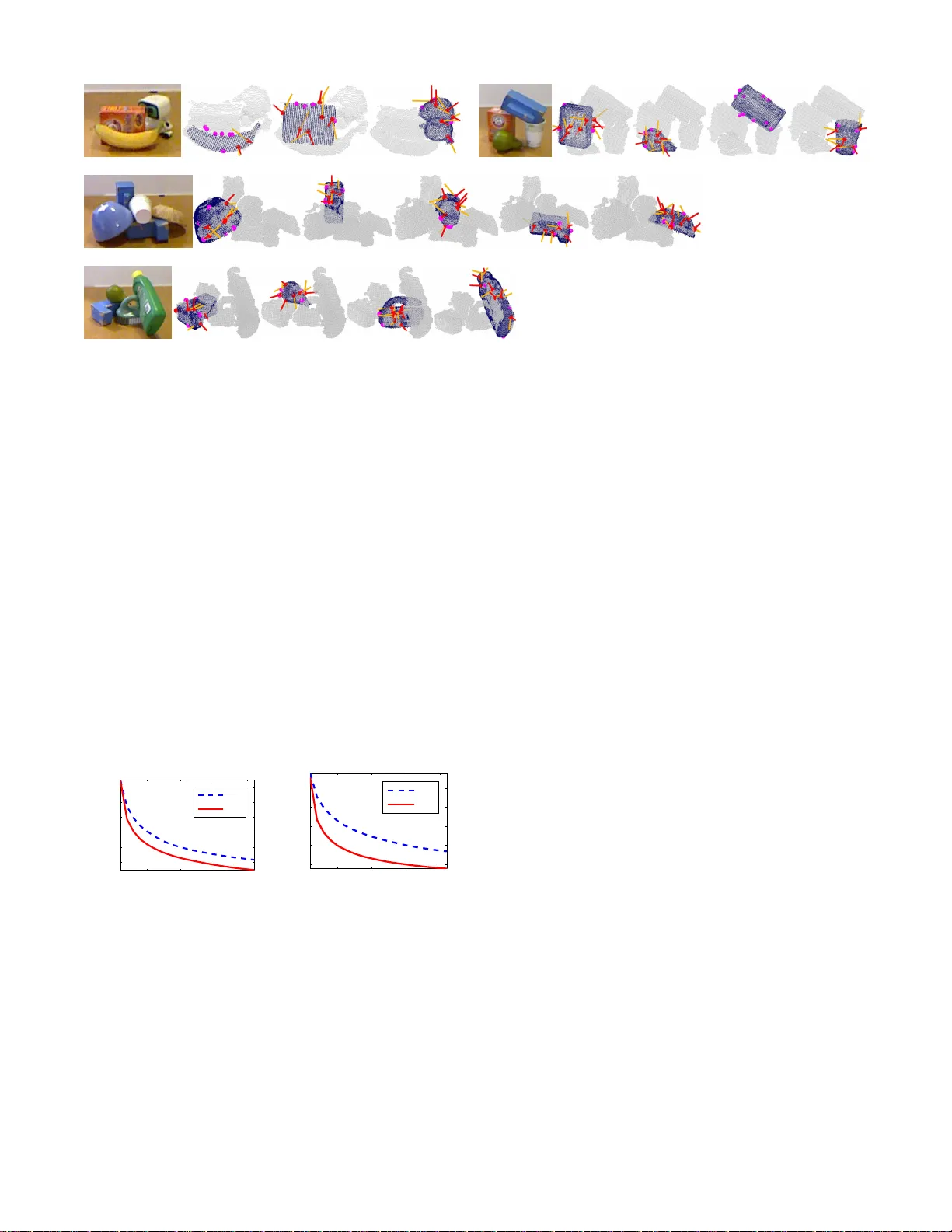
Bingham Pr ocrustean Alignment fo r Object Detection in Clu tter Jared Glover and Sanja Popovic Abstract — A new system f or object detection in cluttered RGB-D images is presented. Our main contribution is a new method called Bingham Procrustean Alignment (BP A) to align models with the scene. BP A uses point corr espondences between oriented features to derive a probability distribution o v er possible mo del poses. The orientation component of this distri- bution, conditioned on the position, is shown to be a B ingham distribution. This result also applies t o the classic pro blem of least-squares alignment of point sets, when point featur es are orientation-less, and giv es a p rincipled, probabilistic way to measure p ose uncertainty in th e rigid alignment p roblem. Our detection system l ev erages BP A to achieve more reliable object detections in clut ter . I . I N T R O D U C T I O N Detecting known, rigid objects in RGB-D images r elies on being able to align 3-D object mod els with an observed scene. If alignments are inconsistent or inaccurate, d etection rates will suffer . In noisy and clutter ed scene s (such as shown in figure 1), goo d alignments must rely on multip le cues, such as 3 -D poin t position s, surface n ormals, c urvature directions, edg es, and ima ge featur es. Y et there is no existing alignment method ( other than bru te f orce optim ization) that can fuse all of this in formatio n t ogether in a mea ningfu l w ay . The Bingham distrib u tion 1 has recen tly been sh own to be useful f or f using o rientation infor mation for 3-D object detection [6]. In this p aper, we derive a surprising result connectin g the Bingham distribution to the classical lea st- squares alignment problem , wh ich allows our new system to easily fu se information fro m bo th position an d orienta- tion inf ormation in a prin cipled, Bayesian alig nment system which we call Bi ngham Procru stean Align ment ( BP A). A. Backgr ound Rigid alig nment of two 3-D po int sets X and Y is a w ell- studied prob lem—one seeks an optimal (q uaternio n) rotation q and translation vector t to minimize an alignment cost function , such as sum of square d er rors between cor respond - ing points on X an d Y . Given known corr esponde nces, t and q can b e fou nd in c losed fo rm with Ho rn’ s m ethod [8]. If corresponden ces a re u nknown, the alignmen t cost func- tion can be specified in terms of sum- of-squa red distances between nearest-neighb or p oints on X and Y , and iterative algorithm s like ICP (Itera ti ve Closest Point) a re guaranteed to reach a local minimu m of th e c ost fun ction [4]. During each itera tion of ICP , Horn’ s metho d is u sed to solve for an optimal t an d q given a current set of co rrespon dences, a nd Computer Science and Artificial Intell igence Laboratory , Massachuset ts Institut e of T echnolog y , Cambridg e, MA 02139 { jglov,sanja } @mit.e du 1 See the appendix for a brief overv ie w. Fig. 1: Object detections found with our system, along with the feature correspondences that BP A used to align the model. Surf ace features are indicated by red points, wit h lines sticking out of them t o indicate orientations ( red f or normals, orange for principal curv at ures). Edge features ( which are orientation-less) are shown by magenta points. then the corresp ondenc es are upd ated using nearest neig hbors giv en the ne w po se. ICP c an b e slow , b ecause it needs to find den se cor respon- dences between the two point sets a t each iter ation. Sub- sampling the point sets can impr ove speed, but only at the cost of accu racy when the d ata is no isy . Ano ther drawback is its sensiti vity to outliers—fo r example wh en it is applied to a clu ttered scen e with segmentation erro r . Particularly because of th e clutter p roblem, many modern approa ches to alignment u se sparse po int sets, wher e one only uses poin ts computed at espe cially uniqu e ke ypoints in the scene. These ke ypoint features can be comp uted from either 2- D (image ) or 3-D (g eometry ) infor mation, a nd of ten include n ot only position s, but also orientations derived from image grad ients, surface normals, princip al curvatures, etc. Howe ver, these o rientations are typically only used in the feature matching an d pose clu stering stages, and are ignored during the alignm ent step. Another limitation is that the resultin g alignmen ts are often based on just a fe w features, with noisy position measuremen ts, and y et ther e is very little work on estima ting confidenc e intervals on the resulting alignments. Th is is especially difficult wh en the features have d ifferent noise models—for example, a featu re foun d on a flat surface will have a g ood estimate of its surface normal, but a high variance principal curvature direction, while a featur e on an object edge may hav e a noisy nor mal, but p recise principal curvature. Id eally , we would like to ha ve a posterior distri- bution over the space of possible alignments, gi ven the data, and we w ould like th at distribution to include inform ation from feature positions and o rientation measuremen ts, g iv en varying no ise mo dels. As we will see in the next section, a full join t distrib ution on t and q is difficult to obtain. Howe ver , in the o riginal least-squares formulation, it is possible to solve for the Fig. 2: Rigid alignment of two poin t sets. optimal t ∗ indepen dently of q ∗ , simply by takin g t ∗ to be the tra nslation which align s the centro ids o f X and Y . Given a fixed t ∗ , solv ing for the optimal q ∗ then becomes tractab le. In a Bayesian analysis of the least-squares align ment p rob- lem, we seek a full d istribution on q given t , not just the optimal value, q ∗ . That way we can assess the confidence of our o rientation estimates, and fuse p ( q | t ) with other sources of orientatio n inf ormation , such as fro m surface normals. Remarkably , gi ven the common assumption of indepen- dent, isotrop ic Gaussian noise on p osition measure ments (which is implicit in the classical least-squares formulation ), we can show that p ( q | t ) is a Bing ham distribution. This result makes it easy to combine th e least-squar es distribu- tion on q | t with other Bing ham distributions fro m featu re orientation s ( or prio r distributions), since the B ingham is a common distribution f or encoding uncertain ty on 3 -D rotations repr esented as unit qu aternions [5], [6], [2]. The mod e of th e least-squ ares Bingham distribution on q | t will be exactly the same as the optimal orientation q ∗ from Horn’ s method. When other sou rces o f orientation informa tion are av ailable, they may bias the distribution away from q ∗ . T hus, it is imp ortant that the concentr ation (in verse variance) par ameters of the Bingh am distributions are accurately estimated for each source of orientation infor- mation, so that this bias is propo rtional to con fidence in the measuremen ts. (See the appendix for an e xample.) W e use our ne w alignmen t method , BP A, to b uild an objec t detection system for known, rigid objects in cluttered RGB-D images. Ou r system combin es informatio n f rom surface and edge feature correspo ndence s to imp rove object alignm ents in clu ttered scenes ( as shown in figu re 1), an d acheives state- of-the- art recogn ition perfo rmance on both an existing Kinect data set [ 1], and o n a new data set containin g far more clutter and pose variability tha n any existing d ata set 2 . I I . B I N G H A M P RO C RU S T E A N A L I G N M E N T Giv en two 3-D po int sets X and Y in on e-to-on e c or- respond ence, we seek a d istribution over the set of rigid transform ations of X , parameterized by a (quaternion) ro- tation q and a translation vecto r t . Assumin g indepen dent Gaussian noise mode ls o n deviations betwee n corr espondin g points on Y an d (transformed ) X , the conditional distrib ution 2 Most existing data sets for 3-D cluttered object detecti on have ve ry limited object pose v aria bilit y (most of the objects are upright), and objects are often easily separable and s upported by the same flat surfa ce. p ( q | t , X , Y ) is proportion al to p ( X , Y | q , t ) p ( q | t ) , where p ( X , Y | q , t ) = Y i p ( x i , y i | q , t ) (1) = Y i N ( Q ( x i + t ) − y i ; 0 , Σ i ) (2) giv en that Q is q ’ s rotation m atrix, and covariances Σ i . Giv en isotropic no ise models 3 on poin t deviations (so that Σ i is a scalar times th e identity m atrix), p ( x i , y i | q , t ) reduces to a 1 -D Gaussian PDF o n the distan ce b etween y i and Q ( x i + t ) , y ielding p ( x i , y i | q , t ) = N ( k Q ( x i + t ) − y i k ; 0 , σ i ) = N ( d i ; 0 , σ i ) where d i depend s on q and t . Now c onsider the triangle form ed by the origin (center of rotation), Q ( x i + t ) an d y i , as sho wn on the left of fig ure 3. By the law of cosines, the square d-distance betwee n Q ( x i + t ) , and y i is d 2 = a 2 + b 2 − ab co s( θ ) , w hich only depen ds on q v ia the ang le θ between the vectors Q ( x i + t ) an d y i . (W e dro p the i - subscripts o n d , a , b , and θ f or brevity .) W e can thus rep lace p ( x i , y i | q , t ) with p ( x i , y i | θ, t ) = 1 Z exp  ab co s( θ ) σ 2  (3) which has the f orm of a V on-Mises distribution on θ . Fig. 3: D istance between corresponding points as a function of orientation. Next, we need to demonstrate ho w θ dep ends on q . W itho ut loss of generality , ass ume that y i points along the axis (1 , 0 , 0) . Whe n this is not the case, the Bingham distribution over q which we deriv e b elow can be post- rotated by any quatern ion wh ich takes (1 , 0 , 0) to y i / k y i k . Clearly , there will be a f amily of q ’ s w hich rotate x i + t to form an angle of θ with y i , since we can compose q with any ro tation about x i + t and the resulting angle with y i will still be θ . T o demon strate wh at this family is, we first let s be a unit quater nion which rotates x i + t onto y i ’ s axis, and let x ′ i = S ( x i + t ) , where S is s ’ s r otation matrix. Then, let r (with rotation matrix R ) be a quaternion that rotates x ′ i to Q ( x i + t ) , so that q = r ◦ s . Because y i and x ′ i point along the axis (1 , 0 , 0) , the first column o f R , ˆ n 1 , will point in the direction of Q ( x i + t ) , and form an angle 3 This is the impli cit assumption in the lea st-squares formulation. of θ with y i , as shown on the right side of figure 3. T hus, ˆ n 1 · (1 , 0 , 0) = ˆ n 11 = cos θ . The rotation m atrix o f qua ternion r = ( r 1 , r 2 , r 3 , r 4 ) is R =  r 2 1 + r 2 2 − r 2 3 − r 2 4 2 r 2 r 3 − 2 r 1 r 4 2 r 2 r 4 +2 r 1 r 3 2 r 2 r 3 +2 r 1 r 4 r 2 1 − r 2 2 + r 2 3 − r 2 4 2 r 3 r 4 − 2 r 1 r 2 2 r 2 r 4 − 2 r 1 r 3 2 r 3 r 4 +2 r 1 r 2 r 2 1 − r 2 2 − r 2 3 + r 2 4  Therefo re, cos θ = ˆ n 11 = r 2 1 + r 2 2 − r 2 3 − r 2 4 = 1 − 2 r 2 3 − 2 r 2 4 . W e can no w make the following claim about p ( x i , y i | q , t ) : Claim 1. Gi ven that y i lies along the (1 , 0 , 0) axis, then the pr obability density p ( x i , y i | q , t ) is propor tional to a Bingham density 4 on q with p arameters Λ = ( − 2 ab σ 2 , − 2 ab σ 2 , 0) and V =  0 0 0 0 0 1 1 0 0 0 1 0  ◦ s = W ◦ s , where “ ◦ ” indicates column-wise quaternion multiplication. Pr oof. T he Bingham density in claim 1 is g iv en by p ( q | Λ , V ) = 1 F exp 3 X j =1 λ j (( w j ◦ s ) T q ) 2 (4) = 1 F exp  − 2 ab σ 2 r 2 3 − 2 ab σ 2 r 2 4  (5) = 1 F ′ exp  ab co s θ σ 2  (6) since ( w j ◦ s ) T q = w j T ( q ◦ s − 1 ) = w j T r , and cos θ = 1 − 2 r 2 3 − 2 r 2 4 . Since (6) is pr oportio nal to (3) , we conclud e that p ( q | Λ , V ) ∝ p ( x i , y i | q , t ) , as claimed. Claim 2. Let s ′ be a quater nion that ro tates (1 , 0 , 0) onto the a xis of y i (for a rbitrary y i ). T hen th e probability den sity p ( x i , y i | q , t ) is p ropo rtional to a Bing ham density on q with parameters Λ = ( − 2 ab σ 2 , − 2 ab σ 2 , 0) and V = s ′ ◦  0 0 0 0 0 1 1 0 0 0 1 0  ◦ s , where “ ◦ ” indicates column-wise quaternion multiplication. As explained above, the distribution on q from claim 1 must simply b e post-rotated by s ′ when y i is not a ligned with th e (1 , 0 , 0) axis. The pr oof is left to the read er . Putting it all togeth er , we fin d that p ( q | t , X , Y ) ∝ Y i Bingham( q ; Λ i , V i ) · p ( q | t ) (7) = Bingham( q ; ˜ Λ , ˜ V ) · p ( q | t ) (8) where Λ i and V i are taken fr om claim 2 , and wh ere ˜ Λ and ˜ V are co mputed from th e for mula for mu ltiplication of Bingham PDFs, which is given in the a ppend ix. Equation 8 te lls us that, in order to u pdate a p rior on q giv en t after da ta points X and Y are observed, one mu st simply multiply the p rior by an app ropriate Bingham ter m. Therefo re, assumin g a Bing ham prior o ver q given t (which includes the u niform distribution), the co nditional posterior, p ( q | t , X , Y ) is the PDF of a Bing ham d istribution. 4 See the appendix for an o verv ie w of the Bingham distri but ion. T o demonstrate this fact, we relied only upo n the assump- tion of independen t isotrop ic Gaussian noise on p osition measuremen ts, which is exactly the sam e assumption mad e implicitly in the least-squares formulation of the op timal alignment prob lem. Th is illustrates a deep and hitherto unknown c onnection be tween least-square s alignment and the Bingham distribution, and pa ves the way for the fu sion of orientation and position measurements in a wide v ariety of application s. A. Incorp orating Orientation Measur ements Now th at we have shown how the orientation informatio n from the least-squ ares alignment of two p oint sets X and Y is encoded as a Bingh am distribution, it becomes trivial to incorpor ate indepen dent orien tation measurements at some or all of th e p oints, provided that the orientatio n noise mod el is Bingham. Given orientatio n measu rements ( O X , O Y ) , p ( q | t , X ,Y , O X , O Y ) ∝ p ( X , Y , O X , O Y | q , t ) · p ( q | t ) = p ( X , Y | q , t ) · p ( O X , O Y | q , t ) · p ( q | t ) . Similarly as in equation 8 , p ( O X , O Y | q , t ) is the product of Bingham distributions fro m co rrespond ing orientation measuremen ts in ( O X , O Y ) , an d so the entire posterior p ( q | t , X , Y , O X , O Y ) is Bin gham ( provided as before that the prio r p ( q | t ) is Bingham ). B. The Alig nment A lgorithm T o inc orpor ate our Bay esian m odel into an iter ativ e ICP- like alignm ent algorith m, one c ould so lve for the max imum a posteriori (MAP) position an d or ientation by ma ximizing p ( q , t | X , Y , . . . ) with respect to q and t . Ho wev er , for probab ilistic completen ess, it is of ten m ore desirable to dr aw samples fro m this p osterior distribution. The joint p osterior distrib u tion p ( q , t | Z ) —where Z con - tains all the measur ements ( X , Y , O X , O Y , . . . )—can be b ro- ken u p into p ( q | t , Z ) p ( t | Z ) . Unfo rtunately , writing d own a closed-for m distribution fo r p ( t | Z ) is d ifficult. But sampling from the join t d istribution is easy with an importan ce sam- pler , by first sampling t from a pro posal distribution—fo r example, a Gaussian center ed on th e optima l least-squ ares translation (that aligns the ce ntroids of X and Y )—then sampling q fr om p ( q | t , Z ) , and the n weigh ting the samples by the r atio of th e tru e posterior (f rom equation 2) and the propo sal distribution (e. g., Gaussian times Bing ham). W e call this sampling alg orithm Bingh am Pro crustean Alignment (BP A). It takes as input a set of (possibly ori- ented) fea tures in o ne-to-o ne corr esponde nce, and r eturns samples f rom the distribution over po ssible alig nments. I n section V, we will show h ow BP A can be inco rporated into an iterative align ment algorithm that re-comp utes feature correspo ndences at each step and u ses BP A to p ropose a new alignmen t given the cor respond ences. I I I . B U I L D I N G N O I S E - A W A R E 3 - D O B J E C T M O D E L S Our first step in building a system to detect kn own, rigid objects—such as the ones in figure 4— is to build complete 3-D mode ls of each object. Howe ver , the end g oal of model Fig. 4: The 18 objects in our ne w Clutter data set. building is not just to estimate an object’ s geom etry correctly . Rather , we seek to pr edict what an RGB-D sen sor would see, from every p ossible vie win g an gle of th e o bject. T o generate such a predictiv e m odel, we will estimate both the most likely observations f rom each v iewing angle, and also the degree of noise predicted in those measurem ents. That way , our detection system will realize that dep th measurements near object boundaries, on r eflectiv e surfaces, or on surfaces at a high obliq ue angle with respect to the cam era, are less reliable than fron t-on m easuremen ts of non -reflective, interior surface points. In our model-building system, we place each object on a servo-controlled turntable in 2-3 resting positions and collect RGB-D images from a stationary Kinect sensor at 10 ◦ turntable incre ments, for a total o f 60- 90 views. W e then fin d the turntable p lane in the dep th images (using RANSAC), and separate obje ct point clouds (on to p of the turn table) from the backg roun d. Next we align each set of 30 scans (taken of the object in a single resting position) by optim izing for the 2- D po sition of the turn table’ s center of rotatio n, with respect to an align ment cost function that measures the sum- of-squar ed nea rest-neighb or d istances from each object scan to e very other scan. W e then u se another op timization to solve for the 6-dof translation + rotation that align s the 2 -3 sets of scans together into on e, global frame of r eference. After the object scans are alig ned, we compute their su r- face no rmals, p rincipal c urvatures, a nd FPFH featur es [10], and we use the th e r atio of princip al curvatures to estimate the (Bing ham) un certainty on the qu aternion orienta tion defined b y nor mals and p rincipal cu rvature directions at each point 5 . W e then use ray-tracing to build a 3-D occu pancy grid m odel, where in addition to the typical probability of occupancy , we also store each 3-D grid cell’ s mean position and norm al, and variance on the norm als in that cell 6 . W e then threshold the occup ancy grid at a n o ccupan cy probab ility of 0 . 5 , and rem ove interio r cells (which can not be seen from any vie wing angle) to obtain a fu ll mod el point clou d, with associated n ormals and normal variance 5 The idea is to capture the orien tatio n uncertai nty on the princ ipal curv ature dire ction by measuring the “flatness” of the observe d surface patch; see the appendix for details. 6 In fact, we store two “vi e w-buc ket s” per cell, ea ch cont ainin g an occupa ncy probability , a position , a normal, and a normal varian ce, since on thin objects lik e cups and bo wls, there may be points on tw o dif ferent surfac es which fa ll in th e same grid ce ll. 0 0.005 0.01 range error 0 0.5 1 0 0.1 0.2 surface angle normal error 0 0.02 0.04 edge distance Fig. 5: Our noise models predict range and normal errors ( standard de viations) as functions of surfa ce angle and edge distanc e (both with respect to the vie wpoint). estimates. W e also compute a distance transform of th is model point cloud, by computin g the distance from t he center of each cell in the occup ancy grid to the n earest m odel point (or zero if the cell co ntains a mod el po int). Next, for a fixed set of 66 vie wing angles across the view-sphere, we estimate ran ge edges—points on th e model where there is a depth d iscontinuity in th e pred icted range image seen f rom that view angle. W e also store th e minimum distance fro m e ach mod el point to a rang e ed ge for each of the 6 6 viewing ang les. U sing these vie w- depend ent edge distances, along with the angles between surface normals and viewpoints, we fit sigmoid models across the wh ole data set to estimate the expected noise on r ange measur ements and normal estimates as functions of (1) edge distance, and (2) surface a ngle, as shown in figure 5. I V . L E A R N I N G D I S C R I M I N AT I V E F E A T U R E M O D E L S F O R D E T E C T I O N Similarly to o ther recent ob ject detection systems, o ur system com putes a set of feature mod el placement sco re function s, in ord er to evaluate ho w well a given model place- ment hy pothesis fits the scene acco rding to different features, such as depth measurements, surface nor mals, edge location s, etc. In our early experiments with object detection u sing the generative o bject models in the previous section, the system was p rone to make mis-classification erro rs, because some objects scored co nsistently higher o n certain featu re scores (presumab ly due to training set bias). Because o f this pro b- lem, we tra ined discriminative, logistic regression models on eac h of th e score com ponen ts using the tur ntable scans with true model placemen ts as positive training examples and a combin ation of correct ob ject / wrong p ose and wrong object / aligned pose as negative examples. Alignm ents o f wrong objects were found by running the full objec t detection system (from the next section) with the wro ng object on the turntable scans. By a dding an (inde penden t) discriminativ e layer to each of th e feature score ty pes, we were able to boost the classification accuracy of our system considerably . V . D E T E C T I N G S I N G L E O B J E C T S I N C L U T T E R The first stages of ou r object detection pipeline are very similar to many oth er state- of-the- art systems for 3-D object detection, with the exception that we rely more heavily on ed ge infor mation. W e are g iv en a s input an RGB-D image, such as f rom a Kinect. If environmen tal information E x t r a c t fe a tu r e s (n o rm a l s, p cs , f p f h s, e d g e s, s u p e r p i xe l s) RGB-D input Prune samples Fig. 6: Single object detection pipeline. is av ailab le, th e im age may b e pre-pr ocessed by anoth er routine to cr op the image to a n area o f interest, an d to lab el backgr ound pixels (e.g., belong ing to a supporting surface). As illustrated in figure 6, our algor ithm starts by esti- mating a dense set o f surface no rmals on the 3-D poin t cloud derived from the RGB-D imag e. Fro m these surface normals, it estimates princ ipal curvatures and FPFH feature s. In addition , it find s and labels three typ es o f edg es: ra nge edges, image edges, and curvature ed ges—points in the RGB-D im age wher e ther e is a dep th discon tinuity , an imag e intensity discontinuity 7 , or high negative cur vature. T his edge informa tion is converted into an edge image, which is formed from a spatially-blur red, weighted average o f the three edg e pixel masks. Intu itiv ely , th is ed ge image is intended to capture the relati ve likeliho od that each point in the image is part of an obje ct boun dary . Then, the algorithm uses k-mean s to over-segment the p oint clo ud based o n po sitions, nor mals, and spatially-blur red colo rs (in CIELAB space) into a set of 3-D super-pixels. Fig. 7: E xamples of objects correctly aligned by B P A with only two corresp ondences . Next, the algor ithm samples possible oriented f eature correspo ndences from the scene to the model 8 . Then, f or each corr esponden ce, a can didate object pose is sampled using BP A. Given a set of sampled model poses from single correspo ndences, we then reject samples fo r wh ich mo re than 20 % of a subset of 500 rand omly-selec ted model points project into free spac e—places wh ere the dif f erence between observed rang e image depth a nd predicted mode l depth is above 5 cm . Next, we r un a pose c lustering stage, whe re we group co rrespon dences togethe r wh ose samp led object poses are within 2 . 5 cm and π / 16 rad ians of on e another . After pose clustering, we re ject any sample with less than two correspo ndences, then re- sample ob ject poses with BP A. 7 W e use the Ca nny edge detector to find image edges. 8 W e currently use only FPFH corresponde nces in the first stage of detec tion as we did not find the addition of other feat ure types, such as SIFT [9] or S HO T [12], to make any dif ferenc e in our detection rates. At this stage, we have a set o f po ssible mo del placemen t hypoth eses, with at least two features correspond ences ea ch. Because BP A uses a dditional orien tation info rmation, two correspo ndences is often all it takes to lock d own a very p re- cise estimate of an object’ s p ose when the cor respond ences are correct (Figu re 7) . W e p roceed with a second rou nd of m odel p lacement validation and rejec tion, th is time using a scoring f unction that includes (1 ) rang e and norma l dif ferences, which are computed by projecting a new subset o f 50 0 randomly- selected model points into the observed ran ge image, (2) visibility—the r atio o f model poin ts in the subset that are unocclu ded, (3 ) edge likelihoo ds, computed by projecting the model’ s edg e po ints fr om the closest stored v iewpoint into the o bserved edge image, and (4) ed ge v isibility— the ratio of edge po ints that ar e unocclu ded. Each of the feature score com ponen ts is com puted as a tru ncated (so as not to over-penalize outliers), a verag e lo g-likelihood o f observed featur es given m odel feature distributions. For score compon ents (1) and (3), we weight the a verag e log-likelihoo d by visibility pro babilities, which are eq ual to 1 if predicted depth < ob served depth, an d N (∆ dep th ; 0 , σ vis ) / N (0; 0 , 1) otherwise 9 . After rejec ting low-scoring samples in r ound 2 , we then refine alignmen ts b y repeating the following th ree steps: 1) Assign ob served super-pixel segments to the mo del. 2) Align mod el to the segments with BP A. 3) Accept the new alig nment if the round 2 model place- ment score has im proved. In step (1 ), we sample a set of assigned segments accord ing to the pro bability that each segment b elongs to the model, which we co mpute as the ratio of segment points (sam pled unifor mly f rom th e segmen t) tha t are within 1 cm in p osition and π / 16 ra dians in norm al orientation fr om the closest model point. In step (2) , we rand omly e xtract a subset of 10 segment p oints from the set of assigned segments, find nearest neighbo r correspond ences from the keypoin ts to the mo del using the model distanc e transform , and then use BP A to align the model to the 10 segment points. Segment po ints are of two types—surface p oints and edge points. W e o nly assign segment ed ge points to model edge points (as pr edicted from the given v iewpoint), and surface 9 W e use σ vis = 1 cm in all of our e xperiments. points to surface points. Figures 1 and 8 show examples of object alignmen ts found after segmen t alignment, where red poin ts (with red no rmal vectors and orang e principal curvature vectors sticking out of them ) in dicate surface p oint correspo ndences, and magenta points (with n o orien tations) are the edg e point correspo ndences 10 . After round 2 alignme nts, the system removes r edunda nt samples (with the same or similar p oses), and then rejects low scorin g samples using the scores found at the end of the segment alignment p rocess. Then , it p erfor ms a final, gradient- based alig nment, which optimizes the mo del po ses with a local h ill-climbing search to d irectly m aximize mode l placement scores. Since this alignment step is by far the slowest, it is critical that the system has perfo rmed as much alignment with BP A and h as rejected as many lo w-scoring samples as po ssible, to reduce the co mputation al burden. Finally , the system perform s a thir d ro und of model placement e valuation, the n sorts the pose samples by score and returns them. This third rou nd of scoring include s s ev eral additional feature scor e compon ents: • Random walk score—starting from a n obser ved poin t correspo nding to the model, take a ran dom walk in the edge image ( to stay within pr edicted object bou ndaries), then measure the distance from the new observed p oint to the closest m odel poin t. • Occlusion edg e score—ev aluate how well mo del oc- clusion ed ges (where the m odel sur face changes f rom visible to occlu ded) fits the obser ved edge ima ge. • FPFH score—comp utes how well observed and mod el FPFH features match . • Segment score—comp utes distances fro m segmen t points to n earest model points. • Segment af finity score—measures how consistent the set of assigned segments is with respect to pred icted object b ounda ries (as measured by th e obser ved edge image, and by d ifferences in segmen t p ositions an d normals). V I . D E T E C T I N G M U LT I P L E O B J E C T S I N C L U T T E R T o detect mu ltiple objects in a scene, we run th e individual object detector from the previous sectio n to obtain the 50 best model placements for each model, along with their individual scores. Then, f ollowing Aldoma et. al [1], we u se simulated annealing to op timize the sub set of model placemen ts (out of 50 × N for N mo dels) accor ding to a multi- object-plac ement score, which we com pute as a weigh ted sum of th e following score com ponen ts: (1 ) the a verag e o f single object scor es, weighted by the nu mber of observed points e ach object explains, (2) the ratio of explained / total ob served points, and (3) a small penalty for th e total numb er of detected objects. W e also keep track o f the top 100 multi-ob ject- placement samples found du ring optimization, so we can return a set of possible scene inte rpretation s to th e user (in the sp irit of inter pretation tree method s [7]). This is particularly u seful for r obot v ision systems b ecause they can use tr acking, prior knowledge, or other sensory inpu t (like 10 In future work, we pla n to inc orporate edge ori entat ions as well. Fig. 9: The Clutter testing data set. touch) to provide add itional v alidation of mod el p lacements, and we don ’t want detectio ns from a single RGB-D image to filter o ut possible mode l p lacements p remature ly . V I I . E X P E R I M E N TA L R E S U LT S W e tested o ur object detectio n system on two Kinect- based data sets—the Kinect data set from Ald oma et. al [1] containing 35 mod els and 50 scenes, and a new , more difficult data set with many mor e o cclusions an d obje ct po se variations that we collected fo r this pap er which we will refer to as Clutter , which contains 18 m odels and 30 scenes (Figure 9). W e used the same parameters ( score comp onent weights, n umber of samples, etc .) on both data sets. In table I, we compare the p recision and recall of the top scene interpretations (mu lti-object-plac ement sam ples) of our method against Aldom a e t. a l on bo th data sets 11 . this paper (BP A) this paper (ICP) A ldoma et. al [1] precisio n recall precisio n recall precision recall Kinect 89.4 86.4 71.8 71.0 90.9 79.5 Clutte r 83.8 73.3 73.8 63.3 82.9 64.2 T ABLE I: A comparison of precision and recall. # samples 1 2 3 5 10 20 recall 73.3 77.5 80.0 80.8 83.3 84.2 T ABLE II: Recall o n the Clutter data set as a fu nction of the number of scene interpretation samples. Our algorithm (with BP A) achieves state-of-th e art recall perfor mance on both d ata sets. When multiple scene in ter- pretations ar e consider ed, we ach ieve even higher recall rates (T able II). Our p recisions are similar to the baseline meth od (slightly high er on Clutter , sligh tly lower on Kinect ). W e were u nable to train discriminative featur e models on the Kinect d ata set, becau se the original tra ining scans were no t provided. T rainin g on scenes th at are mor e similar to th e cluttered test scenes is also likely to impr ove precision on the Clutter data set, since ea ch train ing scan contain ed only one, fully -visible o bject. 11 Since neither ours nor the ba seline method uses colors in their obj ect models, we considere d a model placement “correct” for the Clutter data set if it was within a threshold of the correct pose ( 2 . 5 c m , p i/ 16 radians) with respect to the model’ s symmetry grou p. F or example, we don’t penalize flipping boxes front-to-back or top-to-b ottom, since the resulting differe nce in obje ct appearance is purely non-geometr ic. For the Kine ct data set, we used the same correctness measure as the baseline method (RMSE between model in true pose and esti mated pose), with a threshol d of 1 c m . Fig. 8: Object detections found wit h our system, along with the feature correspondences that BP A used to ali gn the model. Surface features are indicated by red points, with lines sticking out of them to indicate orientations (red for normals, orange for principal curv atures). Edge features (which are orientation-less) are sho wn by magenta points. A. BP A vs. I CP W e ev aluated the be nefits of our new alignme nt method, BP A, in two ways. First, we compare d it to I CP by rep lacing the BP A alig nment step in round 2 with an ICP a lignment step 12 . This resulted in a d rop of 1 0% in bo th precision an d recall on th e Clutter data. For a second test of BP A, we initialized 50 m odel place- ments by add ing random Gaussian noise to th e groun d truth poses for each object in ea ch scene of the Clutter data set. Then, we ran BP A and I CP for 20 iterations on eac h of the mode l placements 13 . W e then compute d the average of the minimu m pose errors in each alignme nt trial, where the minim um at time t in a g iv en trial is com puted as the minimum pose err or from step 1 to step t . (Th e justification for this measure is that this is approximately what the “accept if score improves” step of ro und 2 is doin g.) As shown in figure 10, th e p ose errors decr ease much faster in BP A. 5 10 15 20 0.02 0.022 0.024 0.026 0.028 0.03 alignment iterations X error ICP BPA 5 10 15 20 0.2 0.22 0.24 0.26 0.28 alignment iterations Q error ICP BPA Fig. 10: C omparing BP A with ICP . (Left) The average of the minimum position err ors in each alignmen t t rial. (Right) The av erage of the minimum orientation errors in each alignme nt trial. V I I I . R E L AT E D W O R K Since the re lease of the Kinect in 2010 , much progress has been made o n 3-D o bject dete ction in cluttered RGB- D scenes. T he two most su ccesful systems to date are 12 Both ICP and BP A used the same point correspondences; the only dif ference was that BP A incorporat ed point feature orientat ions, while ICP used only their positions. 13 In other words, we repeated the alignmen t step of round 2 twenty times, rega rdless of whet her the total score improv ed. Aldoma et. al [1] and T ang et. al [1 1]. Aldoma’ s system is purely geom etric, and uses SHOT features [12] for m odel- scene corr esponden ces. It relies heavily on p ose clustering of feature c orrespon dences to suggest mo del place ments 14 . The main contr ibution of Aldo ma’ s system is that th ey jointly optimize multiple model p lacements for consistency , which inspired ou r own m ultiple object detectio n system. T ang’ s detection system uses both g eometry and im age features, an d place d fir st in the ICRA 20 11 So lutions in Per- ception instance recogn ition ch allenge. Their system relies heavily on being able to segment ob jects in the scen e f rom one anoth er , and most of th e effort is spen t on comb ining geometry and image fe atures fo r classification of scen e segments. It is unclear how well the system would perfor m if such se gmentations are no t easy to ob tain, as is the case in our new Clutter data set. The Bingham d istribution w as first used for 3-D c luttered object d etection in Glover et. a l [6 ]. Howe ver , that system was in complete in that it lacked any alig nment step, an d differs greatly fro m this work because it did not use fea ture correspo ndences. I X . C O N C L U S I O N A N D F U T U R E W O R K W e h av e presented a system fo r 3-D clu ttered object detection which uses a ne w alignment method c alled B ing- ham Procru stean Alignmen t (BP A) to impr ove detections in highly clutter ed scene s, along with a new RGB-D data set which co ntains much more clu tter and pose variability th an existing d ata sets. Our system re lies hea vily o n geometry , and will clearly bene fit fr om image and color m odels, su ch as in T ang et. al [11]. Our Clutter data set, while challenging, contains zero ambig uity , in that a human could easily detect all of the objects in their co rrect poses, given enoug h time to stu dy the mod els. An importan t d irection o f future work is to hand le am biguo us scen es, wh ere the parts of objects 14 This is essentially a sparse ve rsion of the Hough tra nsform [3], whic h is limited by the number of visib le fea tures on an object , and is why their recall rates tend to be lo wer than in our system for objects that are hea vily occlude d. that ar e visible are insufficient to p erform un ique alignmen ts, and instead o ne ough t to r eturn distributions over possible model poses. In early experime nts we have perf ormed on this problem , the Bingham d istribution has been a useful too l f or representin g orientation amb iguity . A P P E N D I X The Bingham Distrib utio n. T he Bingham d istribution is common ly used to repr esent uncertainty o n 3-D rotations (in un it quater nion f orm) [2], [5], [ 6]. For qu aternions, its density fun ction (PDF) is gi ven by p ( q ; Λ , V ) = 1 F exp ( 3 X i =1 λ i ( v i T q ) 2 ) (9) where F is a n ormalizin g con stant so that the distrib ution integrates to one over the surface of the unit hype rsphere S 3 , th e λ ’ s are no n-po siti ve ( ≤ 0 ) co ncentration par ameters, and the v i ’ s are o rthogo nal direction vectors. Product of Bingham PDFs. The pro duct of two Bingh am PDFs is given by add ing th eir expon ents: f ( q ;Λ 1 , V 1 ) f ( q ; Λ 2 , V 2 ) = 1 F 1 F 2 exp ( q T ( 3 X i =1 λ 1 i v 1i v 1i T + λ 2 i v 2i v 2i T ) q ) = 1 F 1 F 2 exp  q T ( C 1 + C 2 ) q  (10) After computing th e su m C = C 1 + C 2 in the e xponen t o f equation 10, we com pute th e eigenvectors and eigenv alues of C , and th en subtract off the lowest magnitude eigenv alue from each sp ectral compo nent, so that o nly the eigenvectors correspo nding to the largest 3 eigenv alues (in m agnitude) are kept, an d λ i ≤ 0 ∀ i (as in equation 9). W e use th e open-so urce Bingha m Statistics Library 15 to look up the normalizatio n constant. Estimating the Uncertainty on Feature Orientatio ns. When we extract su rface featu res from depth imag es, we estimate th eir 3-D o rientation s from their normals and prin - cipal curvature dir ections by computing the rotation matrix R = [ n p p ′ ] , where n is the nor mal vector, p is the principal curvature vector, and p ′ is the cross product of n and p . W e take the quaternio n associated with this rotation matrix to be the feature’ s estimated orientation. These orientatio n estimates may be incred ibly noisy , not only du e to typ ical sensing n oise, but because on a flat surface patch th e prin cipal curvature direction is undefin ed and will b e chosen co mpletely at rand om. Therefore it is extremely useful to have an estimate of the unc ertainty on each feature orientatio n that allows for the uncer tainty on the normal direction to differ fro m the uncer tainty on the prin- cipal curvature direction . L uckily , the Bingham d istribution is well suited for this task. T o fo rm such a Bingham distribution, we take th e qu ater- nion associated with R to b e the mode of th e distribution, which is orthog onal to all the v i vectors. Then, we set v 3 15 http:/ /code.goo gle.com/p/bingham to be the quater nion associated with R ′ = [ n − p − p ′ ] , which h as th e sam e n ormal as the m ode, but re versed principal cu rvature direction. In q uaternio n form, reversing the prin cipal cu rvature is equ iv alent to the m apping : ( q 1 , q 2 , q 3 , q 4 ) → ( − q 2 , q 1 , q 4 , − q 3 ) . W e th en take v 1 and v 2 to be unit vectors o rthogo nal to the mode and v 3 (and each oth er). G iv en th ese v i ’ s, th e co n- centration p arameters λ 1 and λ 2 penalize deviations in the normal vector , wh ile λ 3 penalizes de viations in the principal curvature direction. Theref ore, we set λ 1 = λ 2 = κ (we use κ = − 100 in all our experiments in this p aper), an d we use the heu ristic λ 3 = max { 10(1 − c 1 /c 2 ) , κ } , where c 1 /c 2 is the ratio of the principal curvature eig en values 16 . When the surface is com pletely flat, c 1 = c 2 and λ 3 = 0 , so the resulting Bing ham distribution will b e co mpletely unifo rm in the princip al cu rvature dir ection. When the surface is h ighly curved, c 1 ≫ c 2 , so λ 3 will eq ual κ , and deviations in the principal cur vature will be p enalized ju st as mu ch as deviations in the n ormal. R E F E R E N C E S [1] Aitor Aldoma, Federico T ombari, Luigi Di Stef ano, and Markus V incze. A global hypothe ses verifica tion method for 3d object recogni tion. In ECCV 2012 , page s 511 –524. Springer , 2012. [2] Matthe w E Antone . Robust camera pose rec ov ery using stochastic geome try . PhD thesis, Massachusett s Institute of T echnology , Dep t. of Electrical Engineering and Computer Scienc e, 2001. [3] Dana H Ballard. Generali zing the hough transform to detect arbitrary shapes. P atte rn r ecogniti on , 13(2):11 1–122, 1981. [4] P .J. Be sl and N. D. McKay . A method for registra tion of 3-d shapes. IEEE T ransact ions on P attern Analysis and Machin e Intelli genc e , 14:239–25 6, 1992. [5] Christopher Bingham. An antipodally sym metric distrib ution on the sphere. The Annals of Statisti cs , 2(6):1201 –1225, 1974. [6] Jared Glov er , Radu Rusu, and Gary Bradski. Monte carl o pose estimati on with quaternion kerne ls and the bingham distribu tion. In Pr oceed ings of Robotic s: Sci ence and Systems , Los Angeles, CA, USA, June 2011. [7] W Eric L Grimson and T omas L ozano-Pe rez. L ocaliz ing o ve rlappin g parts by searching the interpretat ion tree. P attern Analysis and Mach ine Int ellig ence, IEEE T ransact ions on , (4):46 9–482, 1987. [8] Berthold KP Horn. Closed-f orm solution of absolute orient ation using unit quaternions. JOSA A , 4(4):629–642, 1987. [9] David G Lowe. Object recognition from local scale-in variant feature s. In Compu ter V ision, 1999. The P r oceedings of the Se vent h IEEE Internati onal Confer ence on , volume 2, pages 1150–1157. Ieee, 1999. [10] Radu Bogdan Rusu, Nico Blodo w , and Micha el Beetz. Fast Poin t Feature Histograms (FPFH) for 3D Registrati on. In Pr oceedings of the IEEE Inte rnational Confe r ence on Robot ics and Automation (ICRA) , Ko be, Japan, May 12-17 2009. [11] Jie T ang, Stephen Miller , Arjun Singh, and Piete r Abbeel. A textured object recognitio n pipeli ne for color and depth image data. In Robotics and Auto mation (ICRA ), 201 2 IEEE International Confer ence on , pages 3467–3474. IEEE , 2012. [12] Federico T ombari, Samue le Salti, and Luigi Di Stefan o. Unique signature s of histograms for local surface descri ption. Computer V ision–ECCV 2010 , pages 356–369, 2010. 16 The principa l curv ature direction is comput ed with an eigen- decomposit ion of the cov ariance of normal vectors in a neighborh ood about the feature.