The Resurgence of Instantons in String Theory

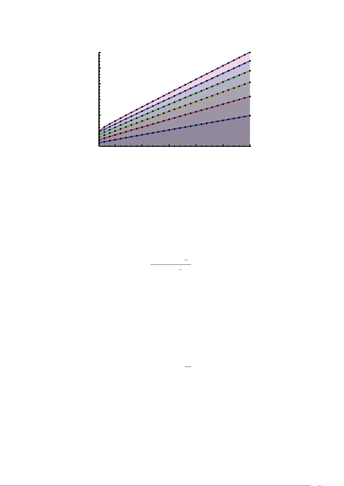
Preprint typeset in JHEP style - HYPER VERSION The Resurgence of Instantons in String Theo ry Inˆ es Aniceto, Rica rdo Schiappa and Marcel V onk CAMGSD, Dep artamento de Matem´ atic a, Instituto Sup erior T´ ecnic o, A v. R ovisc o Pais 1, 1049–001 Lisb o a, Portugal ianiceto@math.ist.utl.pt , schiappa@math.ist.utl.pt , mvonk@math.ist.utl.pt Abstract: Nonperturbative eﬀects in string theory are usually asso ciated to D–branes. In man y cases it can be explicitly sho wn that D–brane instan tons con trol the large–order b eha vior of string p erturbation theory , leading to the w ell–kno wn (2 g )! gro wth of the genus expansion. This paper presen ts a detailed treatmen t of nonp erturbative solutions in string theory , and their relation to the large–order b eha vior of p erturbation theory , making use of transseries and resurgen t analysis. These are pow erful techniques addressing general n onp erturbativ e contributions within non–linear systems, whic h are developed at length herein as they apply to string theory . The cases of topological strings, the P ainlev´ e I equation describing 2d quan tum gravit y , and the quartic matrix model, are explicitly addressed. These results generalize to minimal strings and general matrix mo dels. It is shown that, in order to completely understand string theory at a fully nonp erturbative lev el, new sectors are required b eyond the standard D–brane sector. Keywords: Instan tons, Resurgen t Analysis, T opological and Minimal Strings, Matrix Mo dels . Con tents 1 . In tro duction and Summary 2 2 . Borel Analysis, Resurgence and Asymptotics 6 2.1 Alien Calculus and the Stok es Automorphism 8 2.2 T ransseries and the Bridge Equations 11 2.3 Stok es Constan ts and Asymptotics 15 3 . T op ological Strings in the Gopakumar–V afa Represen tation 18 3.1 T op ological String F ree Energy and Borel Resummation 18 3.2 Simple Resurgence in T opological String Theory 20 4 . The Resurgence of Two–P arameters T ransseries 22 4.1 The Bridge Equations Revisited 24 4.2 Stok es Constan ts and Asymptotics Revisited 29 4.3 Resurgence of the String Gen us Expansion 31 5 . Minimal Mo dels and the Painlev ´ e I Equation 35 5.1 Minimal String Theory and the Double–Scaling Limit 35 5.2 The T ransseries Structure of P ainlev´ e I Solutions 36 5.3 The String Genus Expansion Revisited 42 5.4 Resurgence of Instantons in Minimal Strings 45 5.5 The Nonp erturbative F ree Energy of the (2 , 3) Mo del 56 6 . Matrix Mo dels with P olynomial Poten tials 63 6.1 Matrix Mo dels: Sp ectral Geometry and Orthogonal P olynomials 63 6.2 Resurgence of the Euler–MacLaurin F orm ula 65 6.3 The T ransseries Structure of the Quartic Matrix Mo del 67 6.4 Resurgence of Instantons in Matrix Mo dels and String Theory 73 6.5 The Nonp erturbative F ree Energy of the Quartic Model 84 7 . Conclusions and Outlo ok 90 A . The Painlev ´ e I Equation: Structural Data 93 B . The Quartic Matrix Mo del: Structural Data 95 C . The Double–Scaling Limit: Structural Data 98 D . Stokes Automorphism of Two–P arameters Instanton Series 100 – 1 – 1. In tro duction and Summary String theory may be deﬁned p erturbatively , as a top ological genus expansion, in terms of tw o couplings, α 0 and g s , F ( g s ; { t i } ) ' + ∞ X g =0 g 2 g − 2 s F g ( t i ) , (1.1) where F = log Z is the string free energy and Z the partition function. A t ﬁxed genus g the free energies 1 F g ( t i ) are themselv es p erturbativ ely expanded in α 0 . As it turns out this α 0 expansion is the milder one, with ﬁnite conv ergence radius. What we address in this pap er concerns the top ological genus expansion where one is faced with the familiar string theoretic large–order b eha vior F g ∼ (2 g )! rendering the top ological expansion as an asymptotic expansion [ 1 ]. How can one go b eyond p erturbation theory in g s and deﬁne nonperturbative string theory in general? Stated in this form, this is a very broad and hard question. In order to actually be able to mak e progress on this front w e shall need to sp ecialize to a v ery concrete physical arena—large N duality for top ological strings, matrix mo dels, and their double–scaling limits—where a set of mathematical to ols, whic h go by the name of Borel and resurgen t analysis, will allo w for the construction of solutions to this problem. Let us thus start by reviewing the physical con text. Main Motiv ations P erhaps the most popular approac h to the nonp erturbative deﬁnition of string theory is within the context of large N duality [ 2 ]. In this framework, the partition function of some gauge theoretic system deﬁnes, nonperturbatively , a dual large– N closed–string background. This bac kground is, in turn, describ ed by some geometrical construction which is itself determined b y the particular asymptotic (large N ) limit under consideration. Let us fo cus, for example, on the rather complete picture of [ 3 ]. Here, one starts oﬀ on the gauge theoretic side with a matrix mo del with some p otential, V ( z ), and, giv en a classical v acuum—that is, a distribution of the matrix eigenv alues across the several distinct critical p oin ts of the p otential—, the ’t Ho oft large N limit [ 4 ] yields a (holographic) closed string background which is describ ed by the top ological B–mo del on a sp eciﬁc non–compact Calabi–Y au geometry . It is imp ortan t to notice that diﬀeren t c hoices of classical v acua will yield diﬀerent large N geometries and the same gauge theoretic system will thus allo w for diﬀerent large N asymptotic expansions, represented by these distinct semi–classical geometrical bac kgrounds. No w, the construction of the large N dual in [ 3 ] is essen tially ac hieved by comparing free energies. On the matrix mo del side, the 1 / N ’t Ho oft expansion of the free energy starts oﬀ by a c hoice of a semi–classical saddle–p oin t, described by a sp ectral curve (see, e.g. , [ 5 ] for a review 2 ). Giv en this sp ectral geometry there then exists a w ell–deﬁned procedure to compute the large N expansion of the free energy [ 8 ] which puts the results in [ 3 ] on solid ground, with an explicit construction of the genus expansion ( 1.1 ) of the dual closed string geometry 3 [ 10 ] (which can of course b e chec ked b y explicit calculations strictly within the topological B–mo del closed string theory). 1 In here the t i are geometric mo duli: for instance, in top ological string theory the { t i } mo duli are identiﬁed with K¨ ahler parameters in the A–model and with complex structure parameters in the B–mo del. 2 Let us further point out that this matrix mo del problem of constructing the 1 / N expansion, sp elled out in [ 6 ] and which gained an app ealing geometrical ﬂav or in [ 7 ], has recently b een exactly solv ed purely in terms of sp ectral geometry in [ 8 , 9 ], and that these results lie at the conceptual basis of our description ab ov e. 3 This pro cedure later allow ed for very interesting extensions of the prop osal in [ 3 ] to more general top ological string backgrounds, including duals of closed strings on mirrors of toric backgrounds [ 11 , 12 ]. – 2 – W e ma y now address our main question ab ov e within this physical set–up. In fact, it is also the case that the ’t Ho oft expansion is of the form ( 1.1 ), this time around in p ow ers of N 2 − 2 g but still with F g ∼ (2 g )!, i.e. , the 1 / N expansion is an asymptotic perturbative expansion with zero radius of conv ergence. As w e shall discuss at length in this work, this means that there will be nonp erturbativ e corrections of the form exp ( − N ) that still need to b e taken into consideration. These are asso ciated to instan tons and from a dual closed string p oin t of view, in the large N limit, these corrections t ypically enjoy a semi–classical description corresp onding to D–brane instan ton eﬀects. So we shall see that, giv en a gauge theoretic system and considering one of its p ossible large N limits, one obtains a closed string dual from the semi–classical data of the gauge theory ’t Hooft limit, b oth at perturbative and nonperturbative lev els. This set–up indeed allo ws us to mov e b ey ond the p erturbative ’t Ho oft expansion. One question we address in this w ork is to whic h p oint the nonperturbative description is complete, and whether D–branes account for the full semi–classical nonp erturbative data in such a complete description. That is, if the ﬁnite N gauge theoretic partition function is the correct nonperturbative deﬁnition for closed strings in certain bac kgrounds, one must also understand how this ﬁnite N system enco des, from a dual spacetime p oint of view, all semi–classical nonperturbative contributions. In order to tac kle the aforementioned problems, w e shall need to resort to an extensiv e use of resurgen t analysis. This is a framew ork which allows for the construction of exact nonp ertur- bativ e solutions to rather general non–linear problems in terms of so–called transseries solutions (ﬁrst introduced in the string theoretic context in [ 13 ]), and w e shall further fully dev elop this framew ork as it applies to string theory . T ransseries solutions accoun t for all p ossible saddle– p oin ts of a giv en problem, and denoting them as resurgent essen tially means that the asymptotic b eha vior of the perturbative expansion around some c hosen saddle is dictated by contributions from all other saddles (we shall be precise ab out these ideas in the main b o dy of the text). There are tw o diﬀerent but compleme n tary aspects to these solutions: on the one hand the sp eciﬁc construction of transseries solutions, and the c hec k of their resurgent prop erties, amounts to the mathematical study of either diﬀerential or ﬁnite–diﬀerence equations (in the con text of matrix mo dels and their double–scaling limits). On the other hand, w e also hav e a physical interpre- tation of these solutions: in particular, we shall ﬁnd that these transseries solutions, enco ding the complete nonp erturbative con tent of the large N description, hav e sectors whic h cannot b e asso ciated to D–branes, at least not in a straigh tforw ard fashion (as ﬁrst anticipated in [ 14 , 15 ]). F urther, the resurgen t nonp erturbative solutions ha ve a holographic ﬂav or, in the sense that although one starts from the gauge theoretic (matrix mo del) side, these solutions may b e under- sto o d in terms of dual large N data. Setting up a nonp erturbativ e large N dualit y framework is of ob vious relev ance to man y div erse issues. F or example, a particularly in teresting question is whether going b eyond p erturbation theory around some classical v acuum of the matrix mo del will allow, in the holographic dual, to “see” other closed string backgrounds (which are naturally included in the ﬁnite N gauge theoretic system). Literature Overview In order to place our results in p ersp ective, let us no w present an ov erview of the literature that led up to this w ork. The present research program started in [ 11 , 16 ], which prop osed to generalize many of the nonp erturbativ e results previously obtained within minimal strings to the realm of matrix mo dels oﬀ–criticalit y and top ological strings (intimately related via [ 3 ], as men tioned b efore). Indeed, the double–scaled instan tons unco vered in [ 1 ], and studied from the matrix mo del p oint of view in [ 17 , 18 ], were instrumen tal for, e.g. , the discov ery of D–branes – 3 – in critical string theory 4 spark ed in [ 19 ]. The approac h of [ 16 ] used saddle–p oin t tec hniques to extend results such as [ 17 , 18 , 22 , 23 ] a wa y from criticality . This is an approach that relies on the matrix mo del sp ectral curv e, identifying instantons with B–cycles in the sp ectral geometry , and whic h can also b e extended to the study of multi–instan ton corrections—developed in [ 24 , 15 ], alb eit not very explicitly on what concerns general multi–cut saddle–p oint conﬁgurations. These results were later extended in [ 25 ] to further include instantons asso ciated to A–cycles, which pla y a relev an t role in many top ological string theories (in the so–called c = 1 class). A complemen tary approac h w as in tro duced in [ 13 ], this time around making use of orthogonal p olynomial tec hniques [ 26 ], where transseries were ﬁrst in tro duced to deal with string theoretic problems. One of the results in the present pap er is to fully generalize these ideas to obtain complete nonp erturbativ e solutions to matrix mo dels. In some sense, as we shall make muc h more precise as we go along in this w ork, the transseries approac h amounts to summing ov er al l p ossible bac kgrounds, i.e. , all p ossible distributions of matrix eigenv alues across the many cuts, which corresp ond to all possible large N saddle geometries. In particular, m ulti–instanton corrections within multi–cut geometries [ 24 , 15 ] amount to the exchange of matrix eigenv alues along the diﬀerent cuts, whic h is eﬀectively in terpreted as a change of semi–classical background. This naturally led to the construction of a grand–canonical, manifestly background independent, partition function in [ 27 ] (building upon results in [ 28 , 29 ]) which was further prov ed to b e b oth holomorphic and mo dular cov ariant. Summing ov er all p ossible backgrounds or ov er all p ossible nonp erturbativ e instanton corrections amounts to the same eﬀect. This grand–canonical partition function is built by making use of theta–functions, implying, in particular, that there will be regions in the gauge theory phase diagram where there are no large N expansions ( i.e. , there is no 1 / N expansion due to the oscillatory nature of the theta–functions). This rather imp ortan t idea was later explored, from a large N dualit y p oin t of view, in [ 30 ]. Finally , most of the transseries results extend b eyond the con te xt of matrix mo dels. All they require is the existence of a string equation [ 26 ], typically a ﬁnite diﬀerence equation in the context of oﬀ– critical matrix mo dels, or a diﬀerential equation in the con text of double–scaled minimal strings, whic h is known to also exist in other examples of top ological strings without a very clean matrix mo del relation, e.g. , [ 16 , 31 ]. There may w ell b e larger classes of examples where this is the case. A v ery important role in all this analysis was play ed b y the relation of instantons to the large– order b ehavior of the string p erturbation theory [ 11 , 16 ], i.e. , to the fact that these instan ton eﬀects are testable via their connection to the large–order b eha vior of the 1 / N asymptotic ex- pansion [ 32 ]. Rather impressive agreemen t was found for man y of the calculations in the previous references and this will also b e a very important p oint in the present paper: the resurgent frame- w ork we uncov er, from an analytical approac h, is extensiv ely—and extremely rigorously—tested b y exploring the connections b etw een the asymptotics of multi–instan ton sectors as dictated by resurgence. As we shall explain, resurgence demands for a very tight web of relations in b etw een all these distinct nonp erturbativ e sectors, which is translated into their large–order behavior. These relations ma y b e very thoroughly c heck ed, and to very high precision, making use of n umerical tests, a fact which will clearly justify the construction we shall propose. It might b e fair to sa y that the ﬁrst truly unexp ected result along this line of research app eared in [ 14 ], whic h addressed the large–order asymptotic b eha vior of multi –instanton sectors, rather than just fo cusing on the usual large–order b ehavior of p erturbation theory . In particular, that work addressed the large–order b ehavior of the 2–instantons sector in the P ainlev ´ e I system (the (2 , 3) minimal string) and found that new nonp erturbative sectors, b esides the usual multi– 4 Of course these instan tons also play ed a decisive role in many nonperturbative questions addressed within minimal string theory [ 5 , 20 ] and were later precisely identiﬁed as D–brane conﬁgurations in [ 21 ]. – 4 – instan ton contributions, were required in order to prop erly describ e the full asymptotic b ehavior of this sector. This w as done at leading order, in the resurgen t framew ork, and w as in fact the main motiv ation b ehind the full construction we embrace in our present w ork: to understand the complete set of nonp erturbative contributions demanded by resurgence, within the minimal string context, and further extend it to general matrix mo dels and top ological strings. A t this stage the reader might complain that w e hav e men tioned the w ord “resurgence” a lot but ha ve b een a bit v ague ab out the nature of this framework. This is due to the fact that this formalism, a rather general framew ork introduced in [ 33 ] to address general solutions of non–linear systems in terms of m ulti–instanton data, is a bit in v olv ed. In here, w e wan ted to motiv ate the need for more general approac hes to nonp erturbative issues within large N duality from a purely string theoretic point of view. In section 2 we introduce this formalism (alongside with some new results concerning multi–instan ton asymptotics) and indicate ho w it ma y b e used in string theory . In this wa y we recommend the reader to regard this section as an enlarged introduction to the ideas that are then explored at length in the rest of the paper. Outline of the P ap er This pap er is organized as follo ws. As just mentioned, w e b egin in section 2 with an introduction to resurgence and the developmen t of asymptotic formulae. Asymptotic expansions, with zero radius of conv ergence, need to b e resummed if one is to extract any information out of them. There are, of course, many diﬀerent p ossible ressumation techniques (see, e.g. , [ 34 ]) but since our mo dels deal with asymptotic series which diverge factorially , the natural pro cedure to use in this case turns out to be the Borel resummation framework. This leads in turn to the resurgent framew ork of ´ Ecalle which we introduce in a ph ysical con text in this section. W e also discuss the relation to the Stokes phenomenon; previously discussed in, e.g. , [ 25 , 30 ]. Then, in section 3 , w e apply some of the ideas of resurgence to top ological string theory in the Gopakumar–V afa represen tation [ 35 , 36 ]. This is, essentially , an extension of the work developed in the context of topological strings on the resolv ed conifold in [ 25 ]. Section 4 starts developing the resurgen t framew ork to more general string theoretic systems, in suc h a w ay that w e can apply it to minimal strings and matrix mo dels. This is where we develop the main structure of our nonp erturbative solutions, whic h will later materialize with explicit results in the following sections. In section 5 w e discuss one of our main examples, the (2 , 3) minimal string theory , whic h describ es pure gra vit y in tw o dimensions. In this section we shall construct the full tw o–parameters transseries solution to the P ainlev´ e I equation, generalizing the w ork of [ 14 ]. Do notice that, for the P ainlev ´ e I p erturbative solution, leading asymptotic chec ks ha v e b een carried out in, e.g. , [ 37 , 38 , 39 , 16 ]. A partial transseries analysis was done in [ 40 ]. As for its m ulti–instantons solutions, as mentioned ab o v e, leading asymptotic chec ks hav e b een carried out in [ 14 ]. Our present analysis extends all these partial results to a full general solution. F urthermore, b y analysis of the resulting resurgen t structure we show that this solution has complete nonp erturbative information concerning the minimal mo del. More imp ortantly , in this complete set of nonp erturbative data, and b esides the standard instanton or D–brane sector, we ﬁnd new nonp erturbative sectors with a “generalized” instan ton structure. W e p erform high–precision n umerical tests of al l nonperturbative sectors, including the new “generalized” instan ton sectors, which clearly show the need for all these con tributions in the full exact solution. W e also compute man y , previously unknown, Stok es constan ts of the Painlev ´ e I equation and of the (2 , 3) minimal string theory . In section 6 we analyze the full ﬂedged quartic matrix mo del, starting around the one–cut saddle–p oint geometry . In a similar fashion to what we previously did for the Painlev ´ e I equation, w e construct the transseries solution whic h yields the complete nonperturbative solution to this matrix mo del. W e – 5 – further show ho w this solution relates bac k to the Painlev ´ e I transseries solution in the double– scaling limit. This includes a discussion of the new nonp erturbative sectors of the quartic matrix mo del, alongside with extensive numerical c hecks whic h use the resurgent relations to prov e the v alidit y of these sectors. W e also show that the transseries of the quartic mo del may b e set up in suc h a wa y that the Stok es constants of this problem are essentially giv en by the Stokes constan ts of the (2 , 3) mo del. W e close in section 7 with a discussion and some ideas for future w ork. Do notice that our analysis generated a rather large amoun t of data whic h, for reasons of space, cannot b e all presen ted in the b o dy of this pap er. Mathematic a ﬁles with the relev an t data are a v ailable from the authors up on request. W e do how ever present some partial data in a few app endices, to indicate how the full set–up was constructed. 2. Borel Analysis, Resurgence and Asymptotics One framework to address nonp e rturbativ e completions of rather general non–linear systems is the resurgen t formalism of ´ Ecalle [ 33 ], building upon results of Borel analysis and Stok es phenomena, and w e shall brieﬂy review it in this section 5 . In short, it amounts to a procedure whic h constructs solutions to non–linear problems by addressing all possible m ulti–instanton sectors, i.e. , all p ossible saddle–p oin t conﬁgurations in the path integral. Notice that this means that one constructs the full solution p erturbatively as a p o wer series in the string coupling and also p erturbatively in the instanton num b er, i.e. , as a p ow er series in the (exp onen tial) instan ton contribution—although each instanton con tribution is itself nonperturbative. Besides allo wing for the construction of nonp erturbative solutions, the m ulti–instan ton sectors also allow for a quantitativ e understanding of the large–order b eha vior of the corresp onding p erturbative expansions around a giv en, ﬁxed multi–instan ton sector (the large–order b ehavior of the zero– instan ton sector b eing the simplest case to analyze), a sub ject with a long tradition in quan tum mec hanics and ﬁeld theory , e.g. , [ 41 , 42 , 32 ]. Some ideas of resurgence hav e also b een partially addressed recen tly within the matrix mo del context, see, e.g. , [ 11 , 16 , 13 , 27 , 24 , 25 , 14 , 15 ]. At least in principle, the multi–instan ton information could provide for a reconstruction of the exact free energy , or partition function, in any region of the coupling–constant complex plane. Let us b egin with a rather general introduction to some of these ideas, by considering the free energy in the zero–instan ton sector of any giv en mo del (stringy or not), F ( z ), given as an asymptotic p erturbative expansion 6 in some coupling parameter z (w e will so on tak e z ∈ C ), F ( z ) ' + ∞ X g =0 F g z g +1 . (2.1) Let us assume that, at large g , the co eﬃcients ab ov e b ehav e as F g ∼ g !, rendering the series asymptotic with zero radius of conv ergence. In this case, while we are assuming that F ( z ) exists as a function, one m ust still mak e sense out of the formal pow er series on the righ t–hand–side and w e shall use the notation ' to signal this fact. There are many quantum mec hanical and quantum ﬁeld theoretic examples where this is the typical b ehavior of the p erturbativ e series and this is essen tially due to the gro wth of F eynman diagrams in p erturbation theory [ 32 ]. In the follo wing w e shall explain how resurgen t analysis makes sense of asymptotic series. F or the momen t, let us just mention that the factorial gro wth of the F g is precisely controlled by nonp erturbative 5 The reason for the term “resurgent”—roughly meaning “reapp earing”—will also b e explained in what follo ws. 6 In the following w e shall do p erturbation theory around z ∼ ∞ , rather than g s ∼ 0 as usual. – 6 – instan tons corrections, whic h b ehav e as e − nAz with A denoting the instan ton action and n the in- stan ton n um b er [ 32 ]. As we shall see in great detail, although eac h p erturbative/m ulti–instanton sector is very diﬀerent due to the non–analytic contribution e − nAz (at z ∼ ∞ ), resurgence will relate the asymptotic growth of eac h sector to the leading co eﬃcients of every other sector. Let us no w further p erform a perturbative expansion around the (nonperturbative) con tri- bution at a given ﬁxed instanton num b er. One ﬁnds that the full n –instanton con tribution is of the form (see, e.g. , [ 16 , 13 , 43 , 14 ] for discussions in the con text of matrix mo dels, and top ological and minimal strings) F ( n ) ( z ) ' z − nβ e − nAz + ∞ X g =1 F ( n ) g z g . (2.2) Here β is an exp onen t whic h v aries from example to example 7 , and F ( n ) g is the g –lo op contri- bution around the n –instanton conﬁguration. Let us now further assume that, at large g , these co eﬃcien ts also b eha ve as F ( n ) g ∼ g !, rendering all m ulti–instanton contributions as (divergen t) asymptotic series (just as ab o ve, this is a t ypical b ehavior in man y quantum mec hanical or quan- tum ﬁeld theoretic examples [ 32 ]). As we shall see, it is p ossible to precisely understand the asymptotics, in g , of the m ulti–instan ton contributions F ( n ) g , in terms of the co eﬃcients F ( n 0 ) g , with n 0 close to n . This means that all these asymptotic expansions are resurgent [ 43 ], and w e shall delve into this in the following. As an appro ximation to the exact solution these asymptotic, diver gent formal p ow er series m ust b e truncated and one is consequently faced with the problem that the p erturbativ e expan- sion has zero conv ergence radius. In particular, if we do not know the exact function, F ( z ), but only its asymptotic series expansion, how do w e asso ciate a v alue to the divergen t sum? One framew ork to address issues related to (factorially divergen t) asymptotic series is Borel analysis. In tro duce the Borel transform as the linear map 8 from (asymptotic) p o wer series around z ∼ ∞ to (conv ergen t) p ow er series around s ∼ 0, deﬁned by B  1 z α +1  ( s ) = s α Γ( α + 1) , (2.3) so that the Borel transform of the asymptotic series ( 2.1 ) is the function B [ F ]( s ) = + ∞ X g =0 F g g ! s g , (2.4) whic h “remov ed” the divergen t part of the co eﬃcients F g and renders B [ F ]( s ) with ﬁnite conv er- gence radius around the origin in C . In general, how ever, B [ F ]( s ) will hav e singularities and it is crucial to lo cate them in the complex plane. Indeed, if B [ F ]( s ) has no singularities along a given direction in the complex s –plane, say arg s = θ , one may analytically contin ue this function on the ray e i θ R + and thus deﬁne the inverse Borel transform—or Bor el r esummation of F ( z ) along θ —b y means of a Laplace transform with a rotated con tour as 9 S θ F ( z ) = Z e i θ ∞ 0 d s B [ F ]( s ) e − z s . (2.5) 7 As such, we shall b e more explicit on how to ﬁnd it when we actually address some examples. 8 Notice that the Borel transform is not deﬁned for α = − 1, i.e. , for a constan t term. Thus, in order to Borel transform an asymptotic p ow er series with constant term (denoted the residual co eﬃcient), one ﬁrst drops this constan t term and then p erforms the Borel transform by the rule presen ted ab ov e. 9 If the original asymptotic series one started oﬀ with had a constan t term, dropped in the Borel transform, one ma y now deﬁne the Borel resummation as shown, plus the addition of this constant term. – 7 – The function S θ F ( z ) has, b y construction, the same asymptotic e xpansion as F ( z ) and ma y pro vide a solution to our original question; it asso ciates a v alue to the divergen t sum ( 2.1 ). In the follo wing w e shall further deﬁne the later al Borel resummations along θ , S θ ± F ( z ), as the Borel resummations S θ ±  F ( z ) for  ∼ 0 + . Let us consider a simple example where we take as asymptotic series F ( z ) ' + ∞ X g =0 Γ( g + a ) Γ( a ) 1 A g 1 z g +1 . (2.6) In this case the Borel transform immediately follows as B [ F ]( s ) = 1  1 − s A  a , (2.7) and it has a singularit y (either a pole or a branch–cut, dep ending on the v alue of a ) at s = A . Th us, if the function B [ F ]( s ) has p oles or branc h cuts along its integration con tour ab ov e, from 0 to e i θ ∞ , things get a bit more subtle: in order to p erform the in tegral ( 2.5 ) one needs to choose a con tour whic h av oids suc h singularities. This c hoice of contour naturally introduces an ambiguit y (a nonp erturb ative ambiguit y) in the reconstruction of the original function, whic h renders F ( z ) non –Borel summable. As it turns out, diﬀeren t integration paths produce functions with the same asymptotic b eha vior, but diﬀering b y (non–analytical) exp onentially suppressed terms. It is precisely when there are such obstructions to Borel resummation along some direction θ that the lateral Borel resummations b ecome relev an t: for instance, in the presence of a simple p ole singularity at a distance A from the origin, along some direction θ in C , one may deﬁne the Borel resummation on contours C θ ± , either av oiding the singularit y via the left (as mo ving to w ards inﬁnit y), and leading to S θ + F ( z ), or from the right, and leading to S θ − F ( z ) (see ﬁgure 1 ). One ﬁnds that these t wo functions diﬀer b y a nonperturbative term [ 32 ] S θ + F ( z ) − S θ − F ( z ) ∝ I ( A ) d s e − z s s − A ∝ e − Az . (2.8) F urther nonp erturbativ e am biguities arise as one reconstructs the original function along diﬀer- en t directions (with singularities) in the complex s –plane. As such, diﬀeren t integration paths pro duce functions with the same asymptotic b ehavior, but diﬀering by exp onen tially suppressed terms. T o b e fully precise ab out these, we shall need to delv e into resurgence [ 44 , 45 , 43 ]. 2.1 Alien Calculus and the Stok es Automorphism Let us return to our formal p ow er series ( 2.1 ). This asymptotic expansion is said to b e a simple r esur gent function if its Borel transform, B [ F ]( s ), only has simple p oles or logarithmic branc h cuts as singularities, i.e. , near each singular point ω B [ F ]( s ) = α 2 π i ( s − ω ) + Ψ( s − ω ) log ( s − ω ) 2 π i + Φ( s − ω ) , (2.9) where α ∈ C and Ψ, Φ are analytic around the origin. It can b e shown that simple resurgen t functions allow for the resummation of formal p ow er series along any direction in the complex s –plane, th us leading to a family of sectorial analytic functions {S θ F ( z ) } . F or rigorous details and the pro of of this statement, w e refer the reader to [ 44 , 45 , 43 ]. – 8 – Θ Θ Θ Figure 1: The ﬁrst image shows singularities along some direction θ in the Borel complex plane, and the con tours corresp onding to the left and right lateral Borel resummations along suc h direction. The second and third images show ho w to cross this singular direction, or Stokes line, via the Stokes automorphism: the left Borel resummation equals the right Borel resummation plus the discontin uity of the singular direction (given by the sum ov er Hank el con tours around all singular p oints). As should b e clear—and up to nonp erturbative ambiguities—in diﬀeren t sectors one obtains diﬀeren t resummations and one needs to fully understand Borel singularities in order to “connect” these sectorial solutions together. The next step in order to analyze these Borel singularities in greater detail is to in tro duce ´ Ecalle’s alien calculus [ 33 , 44 ]. A t its basis lies a diﬀeren tial op erator acting on resurgent functions, the alien deriv ative ∆ ω . Let us deﬁne it within the con text of simple resurgen t functions 10 : ∆ ω is a linear diﬀerential op erator from simple resurgent functions to simple resurgent functions, satisfying the Leibniz rule and the following tw o basic prop erties: • If ω is not a singular point (a simple pole or a logarithmic cut), then ∆ ω F ( z ) = 0. • If ω is a singular p oint, let us ﬁrst consider the Borel transform of our resurgen t function ( 2.9 ), which we now conv eniently write as B [ F ]( ω + s ) = α 2 π i s + B [ G ]( s ) log s 2 π i + holomorphic , (2.10) with G ( z ) the resurgen t function whose Borel transform yields Ψ( s ) in ( 2.9 ) (of course in practice it migh t b e hard to ﬁnd G ( z ) explicitly). In this case, the alien deriv ative at a singular p oint ω is given b y S ∆ ω F ( z ) = α + S arg ω G ( z ) . (2.11) T o ha v e a b etter grasp on the calculation of alien deriv atives let us consider another example, sligh tly more inv olv ed than ( 2.6 ), where w e now take as asymptotic series F ( z ) ' + ∞ X g =0 Γ( g + 1) Γ(1) 1 g + 1 1 A g 1 z g +1 . (2.12) It is again very simple to ev aluate the Borel transform as B [ F ]( s ) = − A s log  1 − s A  , (2.13) 10 The deﬁnition for general resurgent functions is more intricate; see, e.g. , [ 44 , 45 , 43 ]. – 9 – with a branc h cut in the complex s –plane running from A to inﬁnit y . It is immediate to c hec k that our asymptotic series ( 2.12 ) deﬁnes a simple resurgent function. F urther noticing that A s = B [ G ]( s − A ) with G ( z ) a resurgen t function closely related to our earlier example ( 2.6 ), G ( z ) ' + ∞ X g =0 Γ( g + 1) Γ(1) 1 ( − A ) g 1 z g +1 , (2.14) it immediately follows by deﬁnition that ∆ A F = − 2 π i G. (2.15) Alien deriv atives thus enco de the whole singular b ehavior of the Borel transform (they enco de ho w muc h B [ F ]( s ) “jumps” at a singularity) and allow for the aforementioned “connection” of sectorial solutions. Indeed, let us consider a singular dir e ction θ , i.e. , a direction along whic h there are singularities in the Borel complex plane. In the original complex z –plane suc h a direction is known as a Stokes line (more on this later). Understanding ho w to connect the distinct sectorial solutions on b oth sides of such direction necessarily entails understanding their “jump” across this direction, and this is accomplished via the Stokes automorphism , S θ , or its related discontin uit y , Disc θ , acting on resurgent functions and satisfying [ 44 ] S θ + = S θ − ◦ S θ ≡ S θ − ◦ ( 1 − Disc θ − ) , (2.16) in suc h a w ay that the action of S θ on resurgen t functions immediately translates in to the required connection of distinct sectorial solutions, across a singular direction θ . In particular, S θ + − S θ − = −S θ − ◦ Disc θ − , (2.17) suc h that Disc θ precisely enco des the full discontin uity 11 of the resurgen t function across θ . Geometrically , one may think of Disc θ − as the sum ov er all Hankel contours which encircle eac h singular p oint in the θ –direction, on the left, and part oﬀ to inﬁnity , on the righ t (see ﬁgure 1 ). The main p oint now is that, as it turns out [ 44 , 45 ], one ﬁnds S θ = exp   X { ω θ } e − ω θ z ∆ ω θ   , (2.18) where { ω θ } denote all singular p oints along the θ –direction. Explicitly , for singularities along the θ –direction in an ordered sequence, one can write [ 45 ] S θ + F ( z ) = S θ − F ( z ) + X r ≥ 1; { n i ≥ 1 } 1 r ! e − ( ω n 1 + ω n 2 + ··· ω n r ) z S θ −  ∆ ω n 1 ∆ ω n 2 · · · ∆ ω n r F ( z )  . (2.19) One concludes that, giv en all p ossible alien deriv ativ es, this result pro vides the necessary con- nection, and thus allo ws for a full construction of the exact nonp erturbative solution alongside with its Riemann surface domain. 11 A function φ satisfying S θ φ = φ , or, equiv alen tly , Disc θ φ = 0, has no Borel singularities along the θ –direction and is known as a r esur genc e c onstant along this direction. In particular, in this region its Borel transform is analytic and φ is thus given b y a conv ergent p o w er series. – 10 – It is rather instructive to explicitly write the Stok es automorphism in our m ulti–instan ton setting. Consider the p ositive real axis, where θ = 0, and where the Borel singularities are lo cated at the multi–instan ton p oints nA with n ∈ N ∗ . In this case: S 0 = exp + ∞ X n =1 e − nAz ∆ nA ! = 1 + e − Az ∆ A + e − 2 Az  ∆ 2 A + 1 2 ∆ 2 A  + · · · . (2.20) This expression will b e rather imp ortan t in what follows. F or the moment let us just go bac k to our earlier example and compute the action of the Stok es automorphism S 0 on ( 2.12 ). Giv en the only non–v anishing alien deriv ativ e of F ( z ), ( 2.15 ), and the fact that higher–order alien deriv ativ es of F ( z ) at A also v anish (as ∆ A G = 0), it is immediate to chec k from ( 2.20 ) ab ov e that S 0 F ( z ) = F ( z ) − 2 π i e − Az G ( z ) . (2.21) Computing alien deriv atives straight from their deﬁnition is a hard task. F ortunately , as we shall see, there are muc h simpler w a ys to compute alien deriv atives. In fact, it turns out that things will greatly simplify b y introducing the p ointe d alien deriv ative ˙ ∆ ω ≡ e − ω z ∆ ω , (2.22) as this op erator commutes with the usual deriv ative [ 45 ],  ˙ ∆ ω , d d z  = 0 . (2.23) W e shall no w turn to explicit computations of alien deriv atives in diﬀerent settings. 2.2 T ransseries and the Bridge Equations Ha ving understoo d the cen tral role that alien deriv ativ es pla y in the construction of nonperturba- tiv e solutions, the question remains: ho w to compute them in a—preferably simple—systematic fashion? The answ er arises in the construction of the bridge e quations , constructing a “bridge” b et w een ordinary and alien calculus. F o cusing on our familiar multi–instan ton setting, with instanton action A (one ma y allo w A to be complex, in which case we shall b e addressing the arg A direction in the Borel complex plane), let us consider a tr ansseries ansatz for our resurgen t function, F ( z , σ ) = + ∞ X n =0 σ n F ( n ) ( z ) , (2.24) where F (0) ( z ) is the formal asymptotic pow er series ( 2.1 ), and where F ( n ) ( z ) = e − nAz Φ n ( z ) , n ≥ 1 , (2.25) are the n –instan ton con tributions ( 2.2 ), as discussed before—the Φ n ( z ) being further formal asymptotic p o w er series. In here, σ is the nonp erturbativ e am biguity or transseries parameter, selecting, in sp eciﬁed wedges of the complex z –plane, distinct nonp erturbative completions to our problem. In the resurgence framework, where transseries also go by the name of resurgent sym b ols along some w edge of the complex plane [ 44 ], this is the most general solution to a given non–linear system. In this work we shall only b e concerned with so–called log–free height–one – 11 – transseries: this means that the ansatz ab ov e is a formal sum of trans–monomials z α e S ( z ) , with α ∈ R and, in our case, S ( z ) a particularly simple conv ergen t series. More general transseries ma y b e constructed, with S ( z ) a transseries itself p ossibly further inv olving comp ositions with exp onen tials or with logarithms, but we refer to [ 46 ] for a complete discussion. It is also imp ortant to realize that the transseries formalism is a rather p o werful technology: when inserted in the non–linear equation satisﬁed by F ( z ) ( e.g. , a ﬁnite–diﬀerence equation in the case of matrix mo dels, or an ordinary diﬀerential equation in the case of minimal strings, as we shall see later), it will yield back the non–linear equation for F (0) ( z )—which is now to be solv ed p erturbatively—; it will yield a line ar and homo gene ous equation for F (1) ( z ); and it will yield line ar but inhomo gene ous equations for F ( n ) ( z ), n ≥ 2. It is thus feasible to solv e for al l mem b ers of this hierarch y of equations and fully compute the transseries solution. Indeed, in all examples of interest to us, it will turn out that all p erturbative co eﬃcients F ( n ) g app earing in the inﬁnite hierarch y of formal asymptotic p ow er series Φ n ( z ) can b e computed by means of (non–linear) recursions. It will b e further the case that the asymptotics of these transseries co eﬃcien ts F ( n ) g will b e exactly determined in terms of neighboring co eﬃcients F ( n 0 ) g , with n 0 close to n , and in terms of a ﬁnite num b er of Stok es constants (deﬁned in the follo wing). Finally , notice that we ha ve assumed the transseries ansatz to dep end on a single parameter, σ , assuming that the resurgent function arises as a solution to some problem dep ending on a single “b oundary condition”. More complicated problems could lead to more general transseries ans¨ atze , and we shall see some such examples further down the line, but for the moment w e just consider the simple case where we may p ow er series expand the transseries ansatz in a single parameter, i.e. , the transseries is an expansion in C [[ z − 1 , σ e − Az ]]. F or simplicit y , we shall further assume that the Φ n ( z ) asymptotic series are simple resurgen t functions. Giv en the p ointed alien deriv ative ˙ ∆ `A = e − `Az ∆ `A , ` ∈ N ∗ , one may now compute ˙ ∆ `A F ( z , σ ) = + ∞ X n =0 σ n e − ( ` + n ) Az ∆ `A Φ n ( z ) . (2.26) The key point is the following: supp ose the transseries F ( z , σ ) is an ansatz for the solution to some diﬀeren tial equation, in the v ariable z . Because the p ointed alien deriv ativ e comm utes with the usual deriv ative, it is straightforw ard to obtain the (linear) diﬀerential equation which ˙ ∆ `A F ( z , σ ) satisﬁes. But, clearly , this will b e the exact same diﬀeren tial equation as the one that ∂ F ∂ σ ( z , σ ) (2.27) satisﬁes—simply b ecause also this deriv ativ e comm utes with the usual deriv ative 12 . Assuming for simplicity that the diﬀeren tial equation is of ﬁrst order, it m ust thus b e the case that ˙ ∆ `A F ( z , σ ) = S ` ( σ ) ∂ F ∂ σ ( z , σ ); (2.28) a relation known as ´ Ecalle’s bridge e quation [ 45 ], relating alien deriv atives to familiar ones! In here S ` ( σ ) is a prop ortionalit y factor which may , naturally , dep end on σ . Recalling that alien 12 In full generality this is slightly more subtle: indeed, it will b e often the case that the diﬀerential equation one is considering will dep end on some other (“initial data”) functions. In this case, for the ab ov e reasoning to hold, these functions m ust either be entire functions, or their Borel transforms cannot ha v e singularities at the points `A (of course these functions will also hav e no dep endence on σ whatsoever; the transseries expression ( 2.24 ) is simply an ansatz for the solution, in tro ducing a new parameter). – 12 – deriv ativ es enco de the singular b eha vior of the Borel transform, the bridge equation tells us that, in some sense, at these singularities we ﬁnd back the original asymptotic p ow er series we started oﬀ with—hence its name as a “resurgen t” function. Let us explore the implications of ( 2.28 ). Sp elling it out as formal p o wer series, and given that Φ n 6 = 0, ∀ n , this immediately implies S ` ( σ ) = 0 , ` > 1 ⇔ ∆ `A F ( z , σ ) = 0 , ` > 1 . (2.29) While one may generically exp ect that the prop ortionality factor S ` ( σ ) has a formal p o w er series expansion as S ` ( σ ) = P + ∞ k =0 S ( k ) ` σ k , homogeneit y in σ of the bridge equation ( 2.28 ) demands k = 1 − ` . One may quickly realize this by introducing a notion of degree such that deg  σ n e mAz  = n + m. (2.30) In this case deg F ( z , σ ) = 0 (which follo ws since F ( z , σ ) only dep ends on σ e − Az ) immediately yields deg S ` ( σ ) = 1 − ` , i.e. , S ` ( σ ) = S ` σ 1 − ` , ` ≤ 1 . (2.31) Plugging this back in to the p ow er series expansion of the bridge equation one ﬁnally obtains a clearer expression for the bridge, or resurgence equations 13 ∆ `A Φ n = ( 0 , ` > 1 , S ` ( n + ` ) Φ n + ` , ` ≤ 1 , (2.32) where we hav e used con ven tions in whic h Φ n v anishes if n is less than zero. This expression yields al l alien deriv atives, in terms of a (p ossibly) inﬁnite sequence of unkno wns S ` ∈ C , ` ∈ { 1 , − 1 , − 2 , · · · } , the so–called analytic inv arian ts of the diﬀerential equation we started oﬀ with. Kno wledge of these analytic in v arian ts allows for a ful l nonp erturbativ e reconstruction of the original function F ( z ), the problem we ﬁrst set out to solv e. How ever, generically , the analytic in v arian ts are transcendental functions of the initial data (say , the diﬀerential equation one started oﬀ with) and quite hard to compute. F or completeness, it is in teresting to notice that the ab o v e resurgence equations ( 2.32 ) may b e translated back to the structure of the Borel transform, at least near eac h singularity `A , by making use of the deﬁnition of alien deriv ative ( 2.11 ) for a simple resurgent function. Indeed, with Φ n ( z ) ' + ∞ X g =1 F ( n ) g z g + nβ and B [Φ n ]( s ) = + ∞ X g =1 F ( n ) g Γ( g + nβ ) s g + nβ − 1 , (2.33) it simply follows via ( 2.10 ) B [Φ n ] ( s + `A ) = S ` ( n + ` ) B [Φ n + ` ] ( s ) log s 2 π i , ` ≤ 1 . (2.34) Going back to the connection formulae ( 2.19 ) or to Stokes’ automorphism ( 2.20 ) makes clear ho w imp ortant ( 2.32 ) is: it is telling us that the somewhat initial multi–instan ton data is enough for a full reconstruction of the nonp erturbativ e solution. Consider ﬁrst the p ositive real axis, where θ = 0, and where the Stokes automorphism is S 0 = exp + ∞ X ` =1 e − `Az ∆ `A ! = 1 + e − Az ∆ A + e − 2 Az  ∆ 2 A + 1 2 ∆ 2 A  + · · · . (2.35) 13 One also obtains a clearer explanation for the name “resurgent”: via the bridge equations the alien deriv ativ es, enco ding the singular b ehavior of the Borel transform, are given in terms of the original asymptotic p o w er series one started oﬀ with (multiplied by suitable Stokes’ constants). – 13 – Giv en the transseries ansatz , the action of S 0 on F ( z , σ ) is en tirely enco ded b y the action of S 0 on the sev eral Φ n ( z ), and this can now be completely determined by the use of the bridge equations ( 2.32 ). But b ecause these v anish whenever ` > 1, the Stokes automorphism immediately simpliﬁes to S 0 = exp  e − Az ∆ A  = 1 + e − Az ∆ A + 1 2 e − 2 Az ∆ 2 A + 1 3! e − 3 Az ∆ 3 A + · · · , (2.36) where (just iterate ( 2.32 )) ∆ N A Φ n = ( S 1 ) N · N Y i =1 ( n + i ) · Φ n + N . (2.37) One may now simply compute S 0 Φ n = + ∞ X ` =0  n + ` n  S ` 1 e − `Az Φ n + ` . (2.38) The in teresting fact ab out the bridge equations ( 2.32 ) is that they con tain m uch more information than just that concerning the p ositiv e real axis. Indeed, consider instead the negativ e real axis, where θ = π , and where the Stokes automorphism b ecomes S π = exp + ∞ X ` =1 e `Az ∆ − `A ! = 1 + e Az ∆ − A + e 2 Az  ∆ − 2 A + 1 2 ∆ 2 − A  + · · · . (2.39) The action of S π on F ( z , σ ) is again entirely enco ded by the action of S π on the sev eral Φ n ( z ), and is determined by the use of the bridge equations ( 2.32 ). All one needs are form ulae for m ultiple alien deriv ativ es, which follow straightforw ardly as 14 N Y i =1 ∆ − ` ( N +1 − i ) A Φ n = N Y i =1 S − ` i · N Y i =1   n − i X j =1 ` j   · Φ n − P N i =1 ` i . (2.40) Notice that the or dering of the alien deriv ativ es in the left–hand side of the expression abov e is rather fundamental, as alien deriv ativ es computed at diﬀer ent singular p oints do not commute. F or example, it is simple to chec k that [∆ − nA , ∆ − mA ] ∝ ( n − m ). Also, b ecause the alien deriv ativ es v anish as soon as one considers ∆ − nA Φ n = 0, this apparent series actually truncates to a ﬁnite sum, at each stage. One may simply compute S π Φ n = Φ n + n − 1 X ` =1 e `Az ` X k =1 1 k ! X ` 1 ,...,` k ≥ 1 P i ` i = `    k Y j =1 S − ` j · k Y j =1 n − j X m =1 ` m !    Φ n − ` (2.41) = Φ n + n − 1 X ` =1 e `Az ` X k =1 1 k ! X 0= γ 0 <γ 1 < ··· <γ k = `   k Y j =1 ( n − γ j ) S − d γ j   Φ n − ` . (2.42) 14 Of course this expression holds as long as n − P N i =1 ` i 6 = 0. As so on as this term v anishes, so do es the multiple alien deriv ative, and consequently so will all subsequent ones. – 14 – In the last line, the sum ov er all p ossible partitions ` i ≥ 1 was replaced by a sum ov er their consecutiv e sums γ s = P s j =1 ` j and w e deﬁned d γ j ≡ γ j − γ j − 1 ( i.e. , the partitions). A few examples of the Stokes automorphism at θ = π are giv en b elow: S π Φ 0 = Φ 0 , (2.43) S π Φ 1 = Φ 1 , (2.44) S π Φ 2 = Φ 2 + S − 1 e Az Φ 1 , (2.45) S π Φ 3 = Φ 3 + 2 S − 1 e Az Φ 2 +  S − 2 + S 2 − 1  e 2 Az Φ 1 . (2.46) Finally , making use of the Stokes automorphism ( 2.18 ), one ma y directly apply the bridge equation ( 2.28 ) in order to ﬁnd, e.g. , S θ + F ( z , σ ) = S θ − exp  ˙ ∆ ω  F ( z , σ ) = S θ − F  z , σ  1 + ω S ω σ − ω  1 ω  . (2.47) In particular, when ω = 1, arg ω = 0, this is S + F ( z , σ ) = S − F ( z , σ + S 1 ) , (2.48) in suc h a wa y that S 1 acts as a Stok es constant for the transseries expression. F or this reason, w e shall generally refer to the analytic in v arian ts S ` as “Stok es constan ts”. Of course this exact same expression could b e obtained by applying the Stokes automorphism at θ = 0, ( 2.38 ), to the transseries ( 2.24 ) (trying the same at θ = π , via ( 2.41 ), w ould b e m uc h more complicated). In the original complex z –plane this Borel–plane singular–direction corresp onds to a Stokes line and what the expression ab ov e describ es is precisely the Stokes phenomena of classical asymptotics— here fully and naturally incorp orated in the resurgence analysis. At a Stokes line, subleading exp onen tials start contributing to the asymptotics and this is accomplished in here b y the “jump” of σ , the c o eﬃcient asso ciated to the transseries formal sum ov er (multi–instan ton) solutions. In other words, the “connection” expression ( 2.19 ) yields a relation b etw een the co eﬃcient(s) in the transseries solution, in diﬀeren t parts of its domain, or, on diﬀeren t sides of the Stokes line. 2.3 Stok es Constan ts and Asymptotics One ma y wonder wh y the long detour in to resurgence and alien calculus. As it turns out, understanding the ful l asymptotic b eha vior of al l multi–instan ton sectors—which is to say , fully understanding the nonp erturbative structure of the problem at hand—demands for this complete formalism. Let us ﬁrst recall the standard large–order dispersion relation that follows from Cauc h y’s theorem [ 32 ]: if a function F ( z ) has a branc h–cut along some direction, θ , in the complex plane, and is analytic elsewhere, it follows F ( z ) = 1 2 π i Z e i θ ·∞ 0 d w Disc θ F ( w ) w − z − I ( ∞ ) d w 2 π i F ( w ) w − z . (2.49) In certain situations [ 41 , 42 ] it is p ossible to show by scaling argumen ts that the in tegral around inﬁnit y does not contribute. In such cases Cauch y’s theorem provides a remark able connection b et w een p erturbative and nonp erturbative expansions. Let us ﬁrst consider our familiar p ertur- bativ e expansion ( 2.1 ), within the transseries set up ( 2.24 ), where F (0) ( z ) = Φ 0 ( z ). In this case, – 15 – the bridge equations ( 2.32 ) tell us, via the Stok es automorphisms ( 2.38 ) and ( 2.41 ), that F (0) ( z ) has the following discontin uities: Disc 0 Φ 0 = − + ∞ X ` =1 S ` 1 e − `Az Φ ` , (2.50) Disc π Φ 0 = 0 , (2.51) i.e. , F (0) ( z ) has a single branch cut along the Stokes direction corresp onding to the p ositive real axis in the Borel complex plane. F rom the p erturbative expansion ( 2.1 ) and using ( 2.49 ) abov e, it immediately follows F (0) g ' + ∞ X k =1 S k 1 2 π i Γ ( g − k β ) ( k A ) g − kβ + ∞ X h =1 Γ ( g − k β − h + 1) Γ ( g − k β ) F ( k ) h ( k A ) h − 1 , (2.52) where w e hav e used the asymptotic expansions for the multi–instan ton contributions ( 2.2 ). It is instructiv e to explicitly write down the ﬁrst terms in this double–series, F (0) g ' S 1 2 π i Γ ( g − β ) A g − β  F (1) 1 + A g − β − 1 F (1) 2 + · · ·  + + S 2 1 2 π i Γ ( g − 2 β ) (2 A ) g − 2 β  F (2) 1 + 2 A g − 2 β − 1 F (2) 2 + · · ·  + + S 3 1 2 π i Γ ( g − 3 β ) (3 A ) g − 3 β  F (3) 1 + 3 A g − 3 β − 1 F (3) 2 + · · ·  + · · · . (2.53) This is the m ulti–instanton generalization of a w ell–known result, also from previous w ork within the matrix mo del and top ological string theory con texts, e.g. , [ 16 , 13 ]. In particular, it relates the co eﬃcien ts of the p erturbativ e expansion around the zero–instanton sector with a sum ov er the co eﬃcien ts of the p erturbativ e e xpansions around all m ulti–instanton sectors, in an asymptotic expansion whic h holds for large g (and p ositive real part of the instanton action). In particular, the computation of the one–lo op one–instan ton partition function determines the leading order of the asymptotic expansion for the perturbative coeﬃcients of the zero–instanton partition function, up to the Stokes factor S 1 . Higher lo op con tributions then yield the successive 1 g corrections. F urthermore, m ulti–instan ton contributions with action nA will yield corrections to the asymptotics of the F (0) g co eﬃcien ts which are exp onentially suppressed as n − g . The no v elty here arises due to the use of alien calculus, which allo ws for a straightforw ard incorp oration of al l multi–instan ton sectors in the asymptotic form ulae, as well as a generalization of this pro cedure to al l multi–instan ton sectors! Indeed, in terms of asymptotics of instan ton series, w e shall ﬁnd that the bridge equations ( 2.32 ) essen tially tell us that, giv en a ﬁxed instan ton sector, its le ading asymptotics are determined by b oth the next and the pr evious instan ton con tributions—at least in examples where a transseries ansatz depending on a single parameter is enough (we shall later see examples where things get more complicated). In particular, at the level of Borel transforms, the singularities closest to the origin, of B [Φ n ]( s ), are lo cated at s = ± A (if n = 0 , 1 there is a single closest–to–the–origin singularit y located at s = A ), and these singularities will necessarily control the large–order b ehavior of the multi–instan ton sectors. Let us now address the full n –instan ton sector. Consider our p erturbativ e expansion ( 2.2 ) within the transseries set–up ( 2.24 ), where F ( n ) ( z ) = e − nAz Φ n ( z ). In this case, the bridge – 16 – equations ( 2.32 ) tell us, via the Stok es automorphisms ( 2.38 ) and ( 2.41 ), that F ( n ) ( z ) has the follo wing discon tin uities: Disc 0 Φ n = − + ∞ X ` =1  n + ` n  S ` 1 e − `Az Φ n + ` , (2.54) Disc π Φ n = − n − 1 X ` =1 e `Az ` X k =1 1 k ! X 0= γ 0 <γ 1 < ··· <γ k = `   k Y j =1 ( n − γ j ) S − d γ j   Φ n − ` , (2.55) i.e. , F ( n ) ( z ) has branc h cuts along the Stokes directions corresp onding to both positive and negativ e real axes in the Borel complex plane. The contribution from the discontin uity at θ = π can also b e rewritten as a sum ov er Y oung diagrams γ i ∈ Γ( k , ` ) : 0 ≤ γ 1 ≤ · · · ≤ γ k = ` of length ` (Γ) = k , and with maximum num b er of b oxes for each part γ i (also called the length of the transp osed Y oung diagram) b eing ` (Γ T ) = ` . This sum is only completely w ell–deﬁned if we also set S 0 , γ 0 ≡ 0, in which case one ﬁnally obtains Disc π Φ n = − n − 1 X ` =1 e `Az ` X k =1 1 k ! X γ i ∈ Γ( k,` )   k Y j =1 ( n − γ j ) S − d γ j   Φ n − ` . (2.56) F or example, consider once again the case n = 3 in the notation ab ov e, Disc π Φ 3 = − e Az X γ i ∈ Γ(1 , 1)  (3 − γ 1 ) S − d γ 1  Φ 2 − e 2 Az 2 X k =1 1 k ! X γ i ∈ Γ( k, 2)   k Y j =1 (3 − γ j ) S − d γ j   Φ 1 . (2.57) Expanding the sums, there will be only one Y oung diagram corresponding to Γ(1 , 1), , for whic h γ 1 = 1. F or Γ(1 , 2) one can only ﬁnd ( γ 1 = 2), while for Γ(2 , 2) there are t wo p ossible Y oung diagrams: ( γ 1 = 1 , γ 2 = 2) and ( γ 1 = γ 2 = 2; but this will not contribute b ecause S 0 = 0). The exp ected result arising from ( 2.46 ) then simply follo ws. F rom the p erturbativ e expansion ( 2.2 ) and the disp ersion relation ( 2.49 ), whic h now needs to account for b oth branc h cuts, it ﬁnally follows F ( n ) g ' + ∞ X k =1  n + k n  S k 1 2 π i · Γ ( g − k β ) ( k A ) g − kβ + ∞ X h =1 Γ ( g − k β − h ) Γ ( g − k β ) F ( n + k ) h ( k A ) h + + n − 1 X k =1    1 2 π i k X m =1 1 m ! X γ i ∈ Γ( m,k )   m Y j =1 ( n − γ j ) S − d γ j      × × Γ ( g + k β ) ( − k A ) g + kβ + ∞ X h =1 Γ ( g + k β − h ) Γ ( g + k β ) F ( n − k ) h ( − k A ) h . (2.58) This expression relates the co eﬃcients of the p erturbativ e expansion around the n –instanton sector with sums ov er the coeﬃcients of the p erturbativ e expansions around al l other m ulti– instan ton sectors, in an asymptotic expansion whic h holds for large g . All Stokes factors are now needed for the general asymptotic problem, and this analysis has essentially b oiled down the asymptotic problem to a problem of precisely computing these Stokes factors. These num b ers – 17 – are transcenden tal inv arian ts of the problem one is addressing and generically hard to compute— although, as we shall see, a matrix mo del computation partially solves this issue. Notice that for instan ton n um b ers n = 0 , 1 the com binatorial factor asso ciated to the Stokes factors S ` at negativ e ` v anishes. As such, the contributions arising from the second and third lines in the expression abov e can only b e seen at instan ton num b er n = 2 and abov e. Finally , let us note that the explicit treatment of the le ading contribution to this type of asymptotics was ﬁrst presented, to the b est of our knowledge, in [ 43 ]. 3. T opological Strings in the Gopakumar–V afa Representation The ﬁrst concrete example we shall explore deals with topological string theory , where the free energy admits an integral Gopakumar–V afa (GV) representation, see [ 35 , 36 ]. Consider the free energy of the A–mo del, on a Calabi–Y au (CY) threefold X , with complexiﬁed K¨ ahler parameters { t i } . As a string theory it satisﬁes the standard top ological gen us expansion ( 1.1 ) where, at gen us g , for large v alues of the K¨ ahler parameters (the large–radius phase), one ﬁnds [ 47 ] F g ( t i ) = + ∞ X d i =1 N g ,d ( X ) e − d · t , (3.1) where the sum is o v er K¨ ahler classes 15 and where the co eﬃcien ts N g ,d ( X ) are the Gromo v–Witten (GW) inv arian ts of X , coun ting world–sheet instantons, i.e. , the n um ber of curv es of genus g and degree d in X . As we men tioned b efore, this α 0 expansion is the milder one with ﬁnite con v ergence radius t c , where the conifold singularit y is reached, whic h may b e estimated from the asymptotic b ehavior of GW inv arian ts at large degree (here γ is a critical exp onent; see, e.g. , [ 31 ]) [ 47 ] N g ,d ∼ d ( γ − 2)(1 − g ) − 1 e d t c , d → + ∞ . (3.2) What we shall b e interested in next is instead the asymptotic genus expansion. In this case, and as throughly in v estigated for the resolved conifold in [ 25 ], the GV in tegral representation for the free energy may b e interpreted as a Borel resummation formula, immediately yielding, as w e will see in the follo wing, the “leading” part of the top ological string resurgent data. 3.1 T opological String F ree Energy and Borel Resummation Let us th us consider the GV integral represen tation for the all–genus top ological string free energy on a CY threefold X , including nonp erturbative M–theory corrections via the type I IA ↔ M / S 1 dualit y [ 36 ] (see also [ 49 , 35 , 50 ] and [ 25 ] for a discussion in the present con text which further highligh ts the Sch winger–lik e nature of this result), F X ( g s ) ' + ∞ X r =0 + ∞ X d i =1 n ( d i ) r ( X ) X m ∈ Z Z + ∞ 0 d s s  2 sin s 2  2 r − 2 exp  − 2 π s g s ( d · t + i m )  . (3.3) In here, the in tegers n ( d i ) r ( X ) are the GV in v ariants of the threefold X , dep ending b oth on the K¨ ahler class d i and on a spin lab el r , and the combination Z = d · t + i m represents the central c harge of certain four–dimensional BPS states [ 36 ]. T o b e completely precise, notice that in 15 d =  d 1 , . . . , d b 2 ( X )  denotes the expansion of the t w o–homology class d on a basis of H 2 ( X , Z ); see, e.g. , [ 48 ]. – 18 – order to obtain the full top ological string free energy one still has to add to this expression the (alternating) constant map contribution [ 51 , 52 ] N g , 0 = ( − 1) g | B 2 g B 2 g − 2 | 4 g (2 g − 2) (2 g − 2)! χ ( X ) , (3.4) where χ ( X ) = 2  h 1 , 1 − h 2 , 1  is the Euler characteristic of X . This term can also b e written as a Borel–like resummation, where the result is 16 [ 35 , 25 ] F d =0 ( g s ) ' + ∞ X g =0 g 2 g − 2 s N g , 0 = 1 2 χ ( X ) X m ∈ Z Z + ∞ 0 d s s  2 sin s 2  − 2 exp  − 2 π s g s i m  . (3.5) Apart from t he ov erall multiplicativ e factor of the Euler c haracteristic, the univ ersal constan t map con tribution has already b een fully addressed in [ 25 ] and we shall th us lea v e it aside for the momen t. Let us fo cus on the GV con tribution ( 3.3 ) instead. By rewriting the sum in m ∈ Z as a sum ov er delta–functions it is simple to obtain the GV formula for the topological string free energy as [ 36 ] F X ( g s ) ' + ∞ X r =0 + ∞ X d i =1 n ( d i ) r + ∞ X n =1 1 n  2 sin ng s 2  2 r − 2 e − 2 π n d · t . (3.6) This makes it quite clear how the input data for a giv en CY threefold is simply its set of GV in teger in v arian ts (and its Euler num b er if one is also to write do wn the constant map contribution). Expressed as a topological genus expansion one ﬁnds, at gen us g , (see, e.g. , [ 51 , 48 , 53 ] for partial expressions) F g ( t i ) = + ∞ X d i =1    | B 2 g | 2 g (2 g − 2)! n ( d i ) 0 + g X h =1 ( − 1) g − h α ( h − 1) g − h +1 (2 g − 2)! n ( d i ) h    Li 3 − 2 g  e − 2 π d · t  , (3.7) where the co eﬃcients α ( n ) m are obtained from the generating function A n ( x ) = (2 n )! Q n k =1 (1 − k 2 x ) ≡ + ∞ X m =0 α ( n ) m +1 x m (3.8) b y p o w er series expansion, and where Li p ( x ) is the p olylogarithm of order p , deﬁned as Li p ( x ) = + ∞ X n =1 x n n p . (3.9) Tw o things to notice are the follo wing: at ﬁxed gen us g , only GV inv ariants n ( d i ) h with h ≤ g con tribute to the free energy [ 36 ]; in particular the “highest” GV inv ariant at gen us g has h = g and appears with co eﬃcien t one in ( 3.7 ) as α ( g − 1) 1 (2 g − 2)! = 1, ∀ g . F urthermore, α (0) g is only non– v anishing when g = 1, implying that n ( d i ) 1 only contributes to the gen us one free energy . What w e w ant to understand in here is ho w or when the GV represen tation ( 3.3 ) ma y b e understoo d as a nonperturbative completion of the free energy gen us expansion ( 3.7 ), in 16 This may also be obtained directly from the GV representation b y simply setting d i = 0 and r = 0 in ( 3.3 ) and prop erly identifying the “degree zero” and “spin zero” GV inv arian t with the Euler n um ber of the CY threefold. – 19 – the sense of resurgen t analysis. F urthermore, one would lik e to understand ho w to relate this nonp erturbativ e completion to the large–order b ehavior of the genus expansion ( 3.7 ) via the use of Stokes’ automorphism. F ollowing the approac h in [ 25 ], we shall interpret the GV integral represen tation for the free energy ( 3.3 ) as a Borel resummation formula ( 2.5 ), for S θ F X ( g s ), in suc h a wa y that, after a simple c hange of v ariables, one obtains B [ F X ]( s ) = + ∞ X r =0 + ∞ X d i =1 n ( d i ) r X m ∈ Z 1 s  2 sin s 4 π ( d · t + i m )  2 r − 2 , (3.10) with the GV representation ( 3.3 ) no w amounting to the statemen t that S θ F X ( g s ) = Z e i θ ∞ 0 d s B [ F X ]( s ) e − s g s . (3.11) This rewriting, of course, required changing the integration with the (in general) inﬁnite sums o v er GV in v arian ts, a pro cedure which is only v alid if there is uniform conv ergence of the partial sums in ( 3.10 ). As we hav e seen before, the sum in m is the milder one. F urthermore, at ﬁxed degree, the sum in r will truncate, i.e. , given a ﬁxed t wo–homology class { d i } , there is r ∗ suc h that n ( d i ) r = 0 for all r > r ∗ [ 54 ]. The real issue concerning uniform con v ergence of the GV Borel transform thus arises when we ﬁx genus and sum ov er degree. In this case one ﬁnds that the asymptotic b ehavior of, for example, the gen us zero GV in v ariants at large degree is [ 55 ] n ( d ) 0 ∼ exp (2 π t 2 (1) · d ) d 3 (log d ) 2 , d → + ∞ , (3.12) where 2 π t 2 (1) is a critical exp onent (for instance, in the example of lo cal P 2 this would b e 2 π t 2 (1) ' 2 . 90759 ... [ 55 ]). This is an exponential growth and, as suc h, in strict v alidity , the results that follo w only hold for threefolds with a ﬁnite num b er of GV in v arian ts, i.e. , without compact four–cycles. This is also in line with the general exp ectations brieﬂy discussed in [ 25 ]. In this con text, the only singularities of the GV Borel transform ( 3.10 ), with s 6 = 0, app ear when r = 0 as the zeroes of the sine (lo cated at ω n = (2 π ) 2 n ( d · t + i m ), n ∈ Z ∗ ). In this case one will only ﬁnd pole singularities and the Borel transform ( 3.10 ) may b e written as B [ F X ]( ω n + s ) = 1 2 π n ( d i ) 0  2 π ( d · t + i m ) n s 2 − 1 2 π n 2 s  + holomorphic , (3.13) near each singular p oint ω n . The (multiple) instan ton action, ω n = nA , is further obtained as A m ( t i ) = (2 π ) 2 ( d · t + i m ) . (3.14) In the following we shall make use of this information in order to explore, from a resurgent p oint of view, when do es the Borel in terpretation of the GV integral represen tation ( 3.10 ) provide for a nonp erturbative completion of the top ological string free energy . 3.2 Simple Resurgence in T op ological String Theory The ﬁrst step in understanding the resurgence of top ological strings is to compute alien deriv a- tiv es. At ﬁrst, this could seem non–trivial as the GV Borel transform ( 3.13 ) is not quite a simple resurgen t function due to the second order p ole. Ho w ever, explicitly ev aluating the diﬀerence of – 20 – lateral Borel res ummations as in ( 2.8 ), one notices that the contribution from this second order p ole is simple to include in the alien deriv ativ e, which now b ecomes, for n ∈ Z ∗ , ∆ nA F X = − i 2 π g s n ( d i ) 0  (2 π ) 2 ( d · t + i m ) n + g s n 2  ≡ Λ n , (3.15) with an added un usual dep endence on the coupling constant. In spite of this, the right–hand side ab o v e is in fact a resurgent constant, in such a w a y that all multiple alien deriv atives v anish. In this case, it is trivial to compute Stokes’ automorphism, ( 2.18 ). Denoting 17 b y θ = arg A , this is S θ F X = F X + + ∞ X n =1 + ∞ X d i =1 X m ∈ Z Λ n · exp  − (2 π ) 2 n ( d · t + i m ) g s  , (3.16) leading to the discontin uity Disc θ F X = i 2 π g s + ∞ X n =1 + ∞ X d i =1 n ( d i ) 0 X m ∈ Z  (2 π ) 2 ( d · t + i m ) n + g s n 2  e − (2 π ) 2 n ( d · t +i m ) g s . (3.17) Finally , making use of the disp ersion relation ( 2.49 ), where one further assumes that the con tribu- tion around inﬁnit y may b e neglected, one may now compute all co eﬃcients in the p erturbative asymptotic expansion of F X , which has the usual genus expansion form ( 1.1 ). F o cusing on the discon tin uity naturally induced b y the GV integral represen tation ( 3.3 ), namely arg s = 0, and follo wing a calculation v ery similar to the one in [ 25 ] for the case of the resolved conifold, it follo ws F X ( g s ) ' + ∞ X g =1 g 2 g − 2 s + ∞ X d i =1 n ( d i ) 0 | B 2 g | 2 g (2 g − 2)! Li 3 − 2 g  e − 2 π d · t  . (3.18) Some commen ts are in order concerning this result. The ﬁrst obvious one is that this do es not fully match against the GV result ( 3.7 ), as it only captures the leading, dominant Bernoulli gro wth of the free energy . While this is certainly the correct exp ectation for an asymptotic form ula in the case of a ﬁnite n umber of GV in v arian ts, one may also ask if it is p ossible to do an y b etter. Of course, if one is to start with the GV Borel transform ( 3.10 ), its singular part ( 3.13 ) will not include any GV inv arian t n ( d i ) r with r 6 = 0 and, as suc h, will never b e able to yield the subleading contributions in ( 3.7 ) unless these should arise from the singularit y at inﬁnity in the Cauc hy disp ersion relation ( 2.49 ). While this is a p ossibilit y , it is also a notoriously diﬃcult case to handle—the singularity at inﬁnit y is an essential singularit y , leading us far from the realm of simple resurgent functions—further departing from the con ven tional set–up of resurgent asymptotics. A t the end of the day this “loss” of GV inv arian ts n ( d i ) r with r 6 = 0 arises from the exchange of integration and inﬁnite sums in ( 3.3 ) to obtain ( 3.10 ) and all it says is that another pro cedure will b e required in order to lo ok b eyond the Bernoulli growth in ( 3.7 ), i.e. , to study the ful l nonp erturbative information of top ological string theory . In other w ords, while the GV in tegral representation is extremely useful in order to solv e topological string theory at the p erturbative level, ( 3.7 ), one needs extra work if one w ants, in general, to obtain a closed form expression for the topological string Borel transform—p ossibly in terms of GV in v ariants. A t this point it might b e useful to mak e a bridge to the case of matrix mo dels with polynomial p oten tials (a sub ject we shall study in detail later in this pap er). F or these, the Gaussian 17 Notice that in the original integration v ariable of ( 3.3 ), therein denoted s , this would corresp ond to θ = 0. – 21 – comp onen t of the p olynomial p otential will induce a con tribution to the free energy whic h also leads to Bernoulli gro wth [ 25 ], rather similar to the one abov e arising from gen us zero GV in v arian ts. F rom a sp ectral curve p oint of view, b oth these contributions are asso ciated to A– cycle 18 instan tons [ 25 ]. Instantons of this t yp e are alwa ys very simple to handle. As describ ed ab o v e, the alien deriv ativ e is essen tially trivial (it equals a resurgen t constant) and at the end of the day the asymptotics is somewhat univ ersal—and certainly muc h simpler than the discussion in the previous section. All m ulti–instanton sectors hav e no non–trivial large–order behavior (their alien deriv atives v anish, their series truncate and their structure is th us rather diﬀerent from the one in ( 2.2 )) and the p erturbative sector is essentially dominated by Bernoulli growth. F or matrix mo dels with p olynomial p oten tials the truly non–trivial resurgen t structure will then b e asso ciated to higher monomials in the p oten tial which will induce diﬀeren t con tributions to the free energy , this time around asso ciated to B–cycle instantons [ 16 ]. More realistic examples of this non–trivial resurgent structure asso ciated to B–cycle instantons will b e discussed next, as w e mov e to the realm of minimal strings and matrix mo dels in the follo wing sections. F or the momen t, let us just notice that, in general, w e still exp ect top ological strings to display full non– trivial resurgence: if one w an ts to see b eyond the Bernoulli gro wth in ( 3.7 ) one will certainly need to ﬁnd a prop er Borel transform, leading to non–trivial alien deriv atives and asymptotic growth of all multi–instan ton sectors. Thus, in general, there will b e b oth A and B–cycle instantons in top ological string mo dels, b oth con tributing to the full instan ton action, and controlling (in turns, dep ending on the absolute v alue of their corresponding actions) the large–order behavior of p erturbation theory at diﬀeren t v alues of the ’t Hooft mo duli, as recently discussed in [ 56 ]. 4. The Resurgence of Two–P arameters T ransseries In order to address broader string theoretic contexts, in particular those inv olving minimal string theory or matrix mo dels, as w e shall study later in this w ork, we now need to generalize the for- malism introduced in section 2 in order to include transseries dep ending on multiple parameters. Let us start oﬀ with some words on the general transseries set–up (see, e.g. , [ 57 ] for a recent review, or, e.g. , [ 58 , 59 ] for more technical accounts). A rank– n system of non–linear ordinary diﬀeren tial equations, d u d z ( z ) = F  z , u ( z )  , (4.1) ma y alw a ys be w ritten, via a suitable c hange of v ariables, in the so–called prepared form [ 57 ]: d u d z ( z ) = − A · u ( z ) − 1 z B · u ( z ) + G  z , u ( z )  . (4.2) Denoting by { α i } i =1 ··· n the eigenv alues of the linearized system, A =  ∂ F i ∂ u j ( ∞ , 0 )  i,j =1 ··· n , (4.3) then, in the expression ab ov e, A = diag ( α 1 , . . . , α n ) and B = diag ( β 1 , . . . , β n ) are diagonal matrices and one further insures that G  z , u ( z )  = O  k u k 2 , z − 2 u  . It is also conv enien t to 18 These are instantons whose action is given by the p erio d of the sp ectral curv e one–form around one of its A–cycles [ 25 ]. They are simpler than B–cycle instantons (almost “universal” as they directly relate to the ’t Ho oft mo duli), whose action is giv en by the p eriod of the sp ectral curve one–form around one of its B–cycles [ 16 ]. – 22 – c ho ose v ariables such that α 1 > 0. Most cases addressed in the literature deal with the non– r esonant case, where the eigen v alues { α i } i =1 ··· n are Z –linearly indep enden t, in man y cases with arg α i 6 = arg α j . This will not b e the case in the present work, as the string theoretic systems we address r esonate . In the ab ov e set–up, a formal transseries solution to our system of diﬀerential equations ( 4.1 ) is given b y [ 57 ] u ( z , σ ) = u (0) ( z ) + X n ∈ N n \{ 0 } σ n z − n · β e − n · α z u ( n ) ( z ) , (4.4) where σ = ( σ 1 , . . . , σ n ) are the transseries parameters, and where b oth the p erturbative con- tribution, u (0) ( z ), as w ell as instan ton and m ulti–instanton 19 con tributions, u ( n ) ( z ), are formal asymptotic p ow er series of the form u ( n ) ( z ) ' + ∞ X g =0 u ( n ) g z g . (4.5) The fact that the systems we shall address in the following resonate no w translates to ∃ n 6 = n 0 | n · α = n 0 · α . (4.6) F urthermore, one often deals with pr op er transseries, where only exponentially suppressed con tri- butions app ear: the eigenv alues α are such that, for some c hosen direction in the complex z –plane, all contributions along this direction with σ i 6 = 0 are exponentially suppressed; R e ( n · α z ) > 0. Again, as ﬁrst pointed out in [ 14 ], if one wishes to fully address the instanton series in a string the- oretic con text one will also hav e to allo w for less studied non–proper transseries. W e th us see that resurgence in string theory is more in tricate than usual, with resonant non–prop er transseries. As we hav e reviewed in section 2 , asymptotic series need to b e Borel resummed in order to extract sensible information from them. Naturally , this will also b e a required step in the construction of a transseries solution to the non–linear diﬀeren tial equation ( 4.1 ), and it follows that [ 58 , 59 ] S θ ± u ( z , σ ± ) = S θ ± u (0) ( z ) + X n ∈ N n \{ 0 } σ n ± z − n · β e − n · α z S θ ± u ( n ) ( z ) , (4.7) is a go o d solution to our problem along a prop er direction (at least for suﬃciently large | z | ). Man y of the concepts introduced in section 2 now hav e a straigh tforward generalization, for instance a simple extension of Stok es’ automorphism ( 2.19 ) where this time around one ma y write S θ + u ( z , σ ) = S θ − u ( z , σ + S ) (4.8) for the crossing of a Stokes line, with S the asso ciated Stok es constants. W e shall no w construct the resurgen t formalism for the speciﬁc case of t wo–parameters transseries, whic h will turn out to b e the required framework to address the instanton series in 2d quan tum gravit y (as ﬁrst uncov ered in [ 14 ] for the case of the Painlev ´ e I equation) as w ell as the instanton series in the quartic matrix model, as w e shall discuss in this work. 19 Linear systems hav e no multi–instan ton sectors. – 23 – 4.1 The Bridge Equations Revisited W e hav e seen in section 2 how the bridge equations allow for a simple ev aluation of alien deriv a- tiv es (up to the determination of the Stokes in v arian ts), ( 2.32 ), and ho w this result then allows for an exact ev aluation of the Stokes automorphism along a singular direction in the Borel complex plane, ( 2.38 ) and ( 2.41 ). W e hav e further seen in section 2 how the discontin uities asso ciated to these singular directions end up determining the full multi–instan ton asymptotics ( 2.58 ) and, in essence, solve the nonp erturbative problem via the use of transseries solutions. In general one requires multi–parameter transseries in order to set up full nonp erturbative solutions which completely encode the multi–instan ton asymptotics. F or the main examples w e shall study in this w ork, the quartic matrix mo del and its double–scaling limit, the P ainlev ´ e I equation, it turns out that a tw o–parameters transseries is required, as we shall see later and as discussed in [ 14 ]. W e shall no w derive the bridge equations in this situation. In particular, we consider the sp ecial case of tw o–parameters transseries where the prepared form eigenv alues are {± A } , with A the instanton action 20 . The transseries ansatz is no w simply F ( z , σ 1 , σ 2 ) = + ∞ X n =0 + ∞ X m =0 σ n 1 σ m 2 F ( n | m ) ( z ) , (4.9) where the p erturbative asymptotic series is F (0 | 0) ( z ) ' + ∞ X g =0 F (0 | 0) g z g +1 ≡ Φ (0 | 0) ( z ) (4.10) and where the generalized m ulti–instanton contributions take the form 21 F ( n | m ) ( z ) ' z − β nm e − n (+ A ) z e − m ( − A ) z + ∞ X g =1 F ( n | m ) g z g ≡ e − ( n − m ) Az Φ ( n | m ) ( z ) . (4.11) The characteristic exp onent is often taken to b e of the form β nm = nβ 1 + mβ 2 , but w e shall also allo w for more general combinations. Ev erything else is a a straightforw ard generalization of the standard result ( 2.2 ) and a simple application of our discussion at the beginning of this section. Because ∃ ( n,m ) 6 =( n 0 ,m 0 ) | n − m = n 0 − m 0 this transseries describ es a resonan t system and it is not to o hard to see that one can mak e the “instanton num b er” explicit by sligh tly reorganizing the previous transseries representation, obtaining F ( z , σ 1 , σ 2 ) = + ∞ X n =0 σ n 1 e − nAz + ∞ X m =0 ( σ 1 σ 2 ) m Φ ( m + n | m ) ( z ) + + ∞ X n =1 σ n 2 e nAz + ∞ X m =0 ( σ 1 σ 2 ) m Φ ( m | m + n ) ( z ) . (4.12) This also introduces a natural notion of degree, deg  σ n 1 σ m 2 e kAz  = n − m + k , (4.13) suc h that the transseries F ( z , σ 1 , σ 2 ) has degree zero. 20 This will b e the relev ant case for b oth the Painlev ´ e I equation and the quartic matrix mo del. 21 In here we are simplifying things a bit: as we shall later discuss in the Painlev ´ e I framework, Φ ( n | m ) ( z ) is not alw a ys a plain formal p ow er series in z but ma y sometimes also include logarithmic pow ers, of the form log k z m ultiplied by formal p o w er series in z . F or clarit y of discussion, we shall pro ceed under this simpler assumption. – 24 – Let us no w consider the p ointed alien deriv ative ˙ ∆ `A = e − `Az ∆ `A , ` ∈ Z ∗ , whic h, as we discussed earlier, comm utes with the usual deriv ativ e. The reasoning of section 2 used in deriving the bridge equation also holds no w, alb eit in the tw o–parameters case the space of solutions to the diﬀerential, or ﬁnite diﬀerence, string equation b ecomes t w o–dimensional [ 14 ] (we shall see this very explicitly in the examples that follo w). It must then b e the case that ˙ ∆ `A F ( z , σ 1 , σ 2 ) = S ` ( σ 1 , σ 2 ) ∂ F ∂ σ 1 ( z , σ 1 , σ 2 ) + e S ` ( σ 1 , σ 2 ) ∂ F ∂ σ 2 ( z , σ 1 , σ 2 ); (4.14) the bridge equation in the tw o–parameters setting. Let us explore its implications. First of all, it is quite simple to notice that this immediately determines the degrees of the prop ortionality factors as deg S ` ( σ 1 , σ 2 ) = 1 − ` and deg e S ` ( σ 1 , σ 2 ) = − 1 − `. (4.15) Because these should b e expressed as formal p ow er series expansions, this further implies S ` ( σ 1 , σ 2 ) = + ∞ X k =max(0 , − 1+ ` ) S ( k +1 − `,k ) ` σ k +1 − ` 1 σ k 2 (4.16) and e S ` ( σ 1 , σ 2 ) = + ∞ X k =max(0 , − 1 − ` ) e S ( k,k +1+ ` ) ` σ k 1 σ k +1+ ` 2 . (4.17) Clearly , there are now a whole lot more Stok es constants than b efore. F or simplicity of notation, and noticing that the Stokes constan ts depend only on the t wo parameters k and ` , we redeﬁne them as S ( k +1 − `,k ) ` ≡ S ( k +1 − ` ) ` and e S ( k,k +1+ ` ) ` ≡ e S ( k +1+ ` ) ` . (4.18) Plugging these expressions back in to the p ow er series expansion of the bridge equation ( 4.14 ) one obtains, after a rather long but straightforw ard calculation, ∆ `A Φ ( n | m ) = min( m,n + ` − 1) X k =max(0 ,` − 1) ( n − k + ` ) S ( k − ` +1) ` Φ ( n − k + ` | m − k ) + + min( m − `,n ) X k =max( − ` − 1 , 0) ( m − k − ` ) e S ( k + ` +1) ` Φ ( n − k | m − k − ` ) , (4.19) v alid for all ` 6 = 0. Lo oking at the ` ≥ 1 case ( ` ≤ − 1 is completely analogous), one ﬁnds ∆ `A Φ ( n | m ) = min( m − ` +1 ,n ) X k =0 ( n − k + 1) S ( k ) ` Φ ( n − k +1 | m − k − ` +1) + + min( m − `,n ) X k =0 ( m − k − ` ) e S ( k + ` +1) ` Φ ( n − k | m − k − ` ) , (4.20) whic h can b e directly compared with equiv alen t expressions from [ 14 ]. In these expressions we ha v e used conv entions in which Φ ( n | m ) v anishes if either n or m are less than zero. As compared to the one–parameter case, ( 2.32 ), the increase in complexit y is evident. Analyzing the bridge – 25 – equations in the form ( 4.19 ), it is not diﬃcult to notice that the cases ∆ `A Φ ( n | m ) and ∆ − `A Φ ( m | n ) with ` > 0 are in timately related. In fact, one can go from one to the other b y p erforming the simple changes ( S a ` , e S b ` ) ↔ ( e S a − ` , S b − ` ) and Φ ( a | b ) ↔ Φ ( b | a ) , where a , b can b e any combination of indices. The same relation can b e seen to extend to the full Stok es automorphisms—changing b et w een the S 0 Φ ( n | m ) and S π Φ ( m | n ) cases—whic h w e shall further discuss in the following. In an y case, the main fo cus of our concern deals with the instanton series, Φ ( n | 0) , where these form ulae b ecome ∆ `A Φ ( n | 0) =      0 , ` > 1 , S (0) 1 ( n + 1) Φ ( n +1 | 0) , ` = 1 , S (1 − ` ) ` ( n + ` ) Φ ( n + ` | 0) + e S (0) ` Φ ( n + ` +1 | 1) , ` ≤ − 1 . (4.21) This result clearly illustrates that in the present situation, unlike the one–parameter case, un- derstanding the asymptotics of the physic al instan ton series necessarily requires the use of the gener alize d multi–instan ton contributions, due to the app earance of the term in Φ ( •| 1) whic h, up on multiple alien deriv ation, will mak e materialize the full generalized instanton sector. As we hav e further seen in section 2 , the bridge equations may also b e translated bac k to the structure of the Borel transform, at least near eac h singularity in the Borel complex plane. In the present case w e hav e to consider, for β nm = nβ 1 + mβ 2 , Φ ( n | 0) ( z ) ' + ∞ X g =1 F ( n | 0) g z g + nβ 1 and B [Φ ( n | 0) ]( s ) = + ∞ X g =1 F ( n | 0) g Γ( g + nβ 1 ) s g + nβ 1 − 1 , (4.22) as well as 22 Φ ( n | 1) ( z ) ' + ∞ X g =1 F ( n | 1) g z g + nβ 1 + β 2 and B [Φ ( n | 1) ]( s ) = + ∞ X g =1 F ( n | 1) g Γ( g + nβ 1 + β 2 ) s g + nβ 1 + β 2 − 1 . (4.23) Then, from ( 4.21 ) ab ov e and the deﬁnition of alien deriv ativ e, it simply follo ws, e.g. , B  Φ ( n | 0)  ( s + `A ) =  S (1 − ` ) ` ( n + ` ) B  Φ ( n + ` | 0)  ( s ) + e S (0) ` B  Φ ( n + ` +1 | 1)  ( s )  log s 2 π i , ` ≤ − 1 . (4.24) The next step is to use the alien deriv ativ es in order to fully construct Stokes’ automorphism, allo wing for a full reconstruction of the nonp erturbativ e solution. Consider ﬁrst the p ositive real axis, where θ = 0, and where the Stok es automorphism is S 0 = exp + ∞ X ` =1 e − `Az ∆ `A ! = 1 + e − Az ∆ A + e − 2 Az  ∆ 2 A + 1 2 ∆ 2 A  + · · · . (4.25) Just like in the one–parameter case of section 2 , given the transseries ansatz , the action of S 0 on F ( z , σ 1 , σ 2 ) is en tirely enco ded b y the action of S 0 on the sev eral Φ ( n | m ) ( z ), and this can no w b e completely determined b y the use of the bridge equations. When fo cusing on the physical instan ton series, and again akin to the one–parameter case of section 2 , the bridge equations ( 4.21 ) v anish whenev er ` > 1, and when ` = 1 both one–parameter ( 2.32 ) and t w o–parameters ( 4.21 ) cases are entirely analogous. Thus, the Stokes automorphism immediately simpliﬁes to S 0 = exp  e − Az ∆ A  = 1 + e − Az ∆ A + 1 2 e − 2 Az ∆ 2 A + 1 3! e − 3 Az ∆ 3 A + · · · , (4.26) 22 In the Painlev ´ e I case there will also b e logarithmic con tributions to Φ ( n | 1) ( z ), which we ignore for the momen t. – 26 – where ∆ N A Φ ( n | 0) =  S (0) 1  N · N Y i =1 ( n + i ) · Φ ( n + N | 0) . (4.27) One may now simply compute S 0 Φ ( n | 0) = + ∞ X k =0  n + k n   S (0) 1  k e − kAz Φ ( n + k | 0) , (4.28) a completely straightforw ard generalization of the one–parameter case ( 2.38 ). The no v elties arise as we turn to the Borel negative real axis, where θ = π , and where the Stok es automorphism b ecomes S π = exp + ∞ X ` =1 e `Az ∆ − `A ! = 1 + + ∞ X ` =1 e `Az ` X k =1 1 k ! X ` 1 ,...,` k ≥ 1 P ` i = ` ∆ − ` k A · · · ∆ − ` 1 A = (4.29) = 1 + e Az ∆ − A + e 2 Az  ∆ − 2 A + 1 2 ∆ 2 − A  + · · · . (4.30) Things are now muc h more complicated than in the simple one–parameter transseries case, as the diﬀeren t terms in S π will mix contributions arising from all Φ ( n | m ) . F rom the expression ab o v e for the Stokes automorphism it b ecomes obvious that, in order to ﬁnd the ﬁnal expression for S π Φ ( n | m ) , one ﬁrst needs to fo cus on determining ∆ − ` k A · · · ∆ − ` 1 A Φ ( n | 0) , with ` j ≥ 1. F or k = 1 , 2, this calculation is pretty straigh tforw ard. Using ( 4.21 ) one can write ∆ − ` 1 A Φ ( n | 0) = ( n − ` 1 ) S (1+ ` 1 ) − ` 1 Φ ( n − ` 1 | 0) + e S (0) − ` 1 Φ ( n − ` 1 +1 | 1) , (4.31) ∆ − ` 2 A ∆ − ` 1 A Φ ( n | 0) = n − 2 X i =1 ` i !  ( n − ` 1 ) S (1+ ` 1 ) − ` 1 S (1+ ` 2 ) − ` 2 + e S (0) − ` 1 S (2+ ` 2 ) − ` 2  Φ ( n − P 2 i =1 ` i | 0 ) + + ( n − ` 1 ) S (1+ ` 1 ) − ` 1 e S (0) − ` 2 + n + 1 − 2 X i =1 ` i ! e S (0) − ` 1 S (1+ ` 2 ) − ` 2 + e S (0) − ` 1 e S (1) − ` 2 ! Φ ( n +1 − P 2 i =1 ` i | 1 ) + +2 e S (0) − ` 1 e S (0) − ` 2 Φ ( n +2 − P 2 i =1 ` i | 2 ) . (4.32) In order to go further and generalize these cases to an arbitrary pro duct of alien deriv atives, one ﬁrst needs to determine ∆ − ` k +1 A Φ ( n + m − P k i =1 ` i | m ) . After some eﬀort one can ﬁnd that ∆ − ` k +1 A Φ ( n + m − P k i =1 ` i | m ) = m +1 X q =0 n + m + 1 − q − k +1 X i =0 ` i ! S ( q + ` k +1 ) − ` k +1 + ( m + 1 − q ) e S ( q ) − ` k +1 ! × × Φ ( n + m +1 − q − P k +1 i =0 ` i | m +1 − q ) , (4.33) where w e hav e set S ( ` i ) − ` i ≡ 0, for any ` i ≥ 1, in order to simplify the ﬁnal result. The general case for the ordered pro duct of k alien deriv ativ es of the form Q k i =1 ∆ − ` k +1 − i A = ∆ − ` k A · · · ∆ − ` 1 A , acting on Φ ( n | 0) , is then given b y k Y i =1 ∆ − ` k +1 − i A Φ ( n | 0) = k X m =0 k Y s =1    s X q s =0 " s − s X i =1 q i ! e S ( q s ) − ` s + n − s X i =1 ` i + s − s X i =1 q i ! S ( ` s + q s ) − ` s # × – 27 – × Θ s − s X i =1 q s !) δ k X i =1 q i , k − m ! Φ ( n + m − P k i =1 ` i | m ) . (4.34) In this expression δ ( n, m ) ≡ δ nm is the usual Kroneck er–delta, the function Θ( x ) is the usual Hea viside step–function Θ( x ) = ( 1 , x ≥ 0 , 0 , x < 0 , (4.35) and once again we se t S ( ` i ) − ` i ≡ 0. A pro of of this result can b e found in app endix D . In the same manner as we hav e done earlier in the one–parameter case for the discon tinuit y at θ = π ( 2.56 ), this result can also be rewritten using a sum o ver Y oung diagrams. T o do so, let us ﬁrst deﬁne δ s = P s i =1 q s + 1, suc h that 0 < δ 1 ≤ δ 2 ≤ · · · ≤ δ k = k − m + 1 and 0 < δ s ≤ s + 1 23 . As explained in section 2 , the set of δ s , with s = 1 , . . . , k , form a Y oung diagram Γ( k , k − m + 1) of lengths ` (Γ) = k and ` (Γ T ) = k − m + 1, with the extra constraint that eac h component δ s ∈ Γ( k , k − m + 1) has a maxim um n umber of s + 1 boxes. As suc h, one may ﬁnally rewrite the ab ov e result as k Y i =1 ∆ − ` k +1 − i A Φ ( n | 0) = k X m =0 X δ s ∈ Γ( k,k − m +1) k Y s =1  ( s + 1 − δ s ) e S ( d δ s ) − ` s + (4.36) + n − s X i =1 ` i + s + 1 − δ s ! S ( ` s + d δ s ) − ` s # Θ ( s + 1 − δ s ) ) Φ ( n + m − P k i =1 ` i | m ) . F or this expression to hold, one still needs to set δ 0 ≡ 1 and e S ( s ) 0 = S ( s ) 0 = S ( ` s ) − ` s = 0 (notice that some of these conditions will only be needed in the follo wing). Due to the complexity of this expression, let us pause for an example. Let us c ho ose the case of k = 2, which we ha ve also describ ed in ( 4.32 ) ab o v e, and see what the sum o ver Y oung diagrams ( 4.36 ) ab ov e yields. One ﬁnds: ∆ − ` 2 A ∆ − ` 1 A Φ ( n | 0) = 2 X m =0 X δ s ∈ Γ(2 , 3 − m ) Θ (2 − δ 1 )  (2 − δ 1 ) e S ( d δ 1 ) − ` 1 + ( n − ` 1 + 2 − δ 1 ) S ( ` 1 + d δ 1 ) − ` 1  × × Θ (3 − δ 2 )  (3 − δ 2 ) e S ( d δ 2 ) − ` 2 + ( n − ` 1 − ` 2 + 3 − δ 2 ) S ( ` 2 + d δ 2 ) − ` 2  Φ ( n + m − P 2 i =1 ` i | m ) . (4.37) The sum ov er Y oung diagrams in this expression is ov er δ s ∈ Γ(2 , 3 − m ), with m = 0 , 1 , 2. F or m = 0, one sums o v er all diagrams δ s ∈ Γ(2 , 3) and there are three p ossible diagrams: , and . But b ecause δ 1 ≤ 2 and δ 2 = 3, only t w o will remain: (where δ 1 = 1) and ( δ 1 = 2). F or m = 1, one sums ov er diagrams δ s ∈ Γ(2 , 2) and there are now t wo p ossible diagrams with δ 2 = 2: ( δ 1 = 1) and ( δ 1 = 2). Finally , for m = 2, one sums o ver diagrams δ s ∈ Γ(2 , 1), which corresp onds to the single diagram: ( δ 1 = δ 2 = 1). Plugging these results bac k in to the expression ab ov e, one easily ﬁnds ( 4.32 ) as expected. There is now enough information in order to completely determine the Stok es automorphism, at θ = π , of the instanton series Φ ( n | 0) . Going back to its deﬁnition ( 4.29 ) and making use of our 23 The reason for adding the one in the presen t deﬁnition of δ s is to make all δ s strictly p ositive, and thus naturally lab eled by some Y oung diagram. – 28 – form ulae for multiple alien deriv atives ( 4.36 ) it follows S π Φ ( n | 0) = Φ ( n | 0) + + ∞ X ` =1 e `Az ` X k =1 1 k ! X ` 1 ,...,` k ≥ 1 P ` i = ` ∆ − ` k A · · · ∆ − ` 1 A Φ ( n | 0) = (4.38) = Φ ( n | 0) + + ∞ X ` =1 e `Az ` X k =1 1 k ! X ` 1 ,...,` k ≥ 1 P ` i = ` k X m =0 X δ s ∈ Γ( k,k − m +1) (4.39) k Y s =1 (" ( s + 1 − δ s ) e S ( d δ s ) − ` s + n − s X i =1 ` i + s + 1 − δ s ! S ( ` s + d δ s ) − ` s # Θ ( s + 1 − δ s ) ) · Φ ( n − ` + m | m ) . In terestingly enough, if we further deﬁne γ s = P s i =1 ` i , then the sum ov er the ` i can also b e rewritten as a sum of Y oung diagrams γ i ∈ Γ( k , ` ) : 0 < γ 1 ≤ · · · ≤ γ k = ` ; as long as we set e S ( s ) 0 = S ( s ) 0 = 0. In this case, one ﬁnally obtains the simpler expression S π Φ ( n | 0) = Φ ( n | 0) + + ∞ X ` =1 ` X k =1 e `Az k ! X γ i ∈ Γ( k,` ) k X m =0 X δ s ∈ Γ( k,k − m +1) (4.40) k Y s =1 nh ( s + 1 − δ s ) e S ( d δ s ) − d γ s + ( n − γ s + s + 1 − δ s ) S ( d γ s + d δ s ) − d γ s i Θ ( s + 1 − δ s ) o · Φ ( n − ` + m | m ) . Some commen ts are no w in order. Comparing the Stok es automorphism of the instanton series at the θ = π discontin uit y , for b oth the one–parameter ( 2.56 ) 24 and the tw o–parameter cases (ab o v e), one can see the that the increased degree of complexit y of the latter is translated in the fact that there is no w a sum o ver two indep endent sets of Y oung diagrams (instead of summing o v er just one set of diagrams as in the one–parameter case). It is thus natural to infer that for a general ` –parameter transseries ansatz suc h sums would b e substituted by sums o v er ` indep enden t sets of Y oung diagrams. It is also not too diﬃcult to see that one can reco ver the one–parameter result ( 2.56 ) starting from ( 4.40 ) ab ov e, b y simply setting δ s = s + 1 for all δ s . This corresp onds to c ho osing the Y oung diagrams δ s ∈ Γ( k , k + 1) (with m = 0 and consequently ` ≤ n ) where each ro w has one more b ox than the previous one, e.g. , for k = 4. 4.2 Stok es Constan ts and Asymptotics Revisited The main outcome of the ab ov e calculations are expressions for the discontin uities of the full, ph ysical, multi–instan ton series, enco ded in the Stokes automorphism of Φ ( n | 0) , in b oth θ = 0 , π , directions. As w e ha ve seen earlier, in section 2 , these discontin uities lie at the basis of un- derstanding the full asymptotic b ehavior of all m ulti–instanton sectors and w e shall next use these new Stok es’ discontin uities in order to generalize our results on asymptotics, from the one–parameter to the tw o–parameters case. Recall that by making use of Cauch y’s theorem a giv en function F ( z ) with a branch–cut along some direction θ in the complex plane (and ana- lytic elsewhere) can actually b e fully describ ed precisely by its discontin uity along that direction ( 2.49 ), at least as long as its b ehavior at inﬁnit y do es not contribute. In the presen t case of inter- est, the m ulti–instan ton free energies F ( n | 0) ( z ), which are the co eﬃcients of the tw o–parameters 24 Recall that S θ = 1 − Disc θ . – 29 – transseries ansatz ( 4.9 ), hav e asymptotic expansions giv en by ( 4.10 ) for the p erturbative se- ries and by ( 4.11 ) for the generalized multi–instan ton contributions. Their discontin uities are essen tially giv en b y the Stokes automorphisms of Φ ( n | 0) ( z ) previously calculated. Let us ﬁrst lo ok at the perturbative expansion ( 4.10 ). The discon tinuities of F (0 | 0) ( z ) arise directly from the bridge equations ( 4.21 ), via the Stokes automorphisms ( 4.28 ) and ( 4.40 ), Disc 0 Φ (0 | 0) = − + ∞ X k =1  S (0) 1  k e − kAz Φ ( k | 0) , (4.41) Disc π Φ (0 | 0) = − + ∞ X k =1  e S (0) − 1  k e kAz Φ (0 | k ) . (4.42) Note that F (0 | 0) ( z ) will no w hav e t wo branc h cuts in the Borel complex plane (instead of only one as in the one–parameter transseries case), along b oth p ositiv e and negative real axes. By using ( 4.10 ), ( 4.11 ) and ( 2.49 ) it is not diﬃcult to ﬁnd the asymptotic co eﬃcients of the p erturbative expansion to b e given b y F (0 | 0) g ' + ∞ X k =1  S (0) 1  k 2 π i Γ ( g − β k, 0 ) ( k A ) g − β k, 0 + ∞ X h =1 Γ ( g − β k, 0 − h + 1) Γ ( g − β k, 0 ) F ( k | 0) h ( k A ) h − 1 + + + ∞ X k =1  e S (0) − 1  k 2 π i Γ ( g − β 0 ,k ) ( − k A ) g − β 0 ,k + ∞ X h =1 Γ ( g − β 0 ,k − h + 1) Γ ( g − β 0 ,k ) F (0 | k ) h ( − k A ) h − 1 . (4.43) As should b e by now exp ected, we ﬁnd that the co eﬃcients of the p ertubativ e expansion around the zero–instan ton sector are giv en b y an asymptotic double–sum expansion, v alid for large v alues of g , o v er the co eﬃcients of the p erturbative expansions around (some of ) the generalized m ulti– instan ton sectors. The no velt y in here, as compared to the one–parameter case of section 2 , is that this expansion includes not only the co eﬃcients of the ph ysical instanton series F ( n | 0) g , asso ciated with p ositive real part of the instanton action, but also the generalized co eﬃcien ts F (0 | n ) g , asso ciated with negative real part of the instanton action. In particular, the leading order of this ze ro–instan ton asymptotic expansion is determined by the co eﬃcients of the one–loop (generalized) one–instan ton partition functions, but now up to tw o Stok es constants, namely S (0) 1 and e S (0) − 1 . Higher lo op con tributions will arise as 1 g corrections, while other m ulti–instanton con tributions, with action ± nA , will yield corrections suppressed as n − g . Th us, what we hav e found in the present tw o–parameters transseries setting is that, such as in the one–parameter case, through the use of alien calculus and the bridge equations it is p ossible to include al l multi–instan ton sectors in the asymptotics of the p erturbativ e zero– instan ton sector. F urthermore, through essen tially the same metho ds it is also straightforw ard to generalize this asymptotic result to al l multi–instan ton sectors. This is what w e shall do next for the n –instan ton sector, F ( n | 0) ( z ). Using the form ulae for the Stok es automorphism in the directions θ = 0 , π , of Φ ( n | 0) , given in ( 4.28 ) and ( 4.40 ), we can easily ﬁnd the related discon tin uities in the said directions. As usual, F ( n | 0) ( z ) has branc h cuts in the Stokes directions corresp onding to b oth p ositiv e and negative real axes in the Borel complex plane. Then, b y means of ( 2.49 ) and ( 4.11 ), in particular the iden tiﬁcation F ( n | m ) ( z ) = e − ( n − m ) Az Φ ( n | m ) ( z ), a length y but straighforward calculation leads to (it migh t b e interesting for the reader to compare – 30 – this expression against its one–parameter counterpart, ( 2.58 )) F ( n | 0) g ' + ∞ X k =1  n + k n  ( S (0) 1 ) k 2 π i · Γ ( g + β n, 0 − β n + k, 0 ) ( k A ) g + β n, 0 − β n + k, 0 + ∞ X h =1 Γ ( g + β n, 0 − β n + k, 0 − h ) Γ ( g + β n, 0 − β n + k, 0 ) F ( n + k | 0) h ( k A ) h + + ∞ X k =1    1 2 π i k X m =1 1 m ! m X ` =0 X γ i ∈ Γ( m,k ) X δ j ∈ Γ( m,m − ` +1)   m Y j =1 Σ( n, j )      × × Γ ( g + β n, 0 − β n + ` − k,` ) ( − k A ) g + β n, 0 − β n + ` − k,` + ∞ X h =1 Γ ( g + β n, 0 − β n + ` − k,` − h ) Γ ( g + β n, 0 − β n + ` − k,` ) F ( n + ` − k | ` ) h ( − k A ) h , (4.44) where we hav e introduced Σ( n, j ) =  ( j + 1 − δ j ) e S ( d δ j ) − d γ j + ( n − γ j + j + 1 − δ j ) S ( d γ j + d δ j ) − d γ j  Θ ( j + 1 − δ j ) . (4.45) Recall that we ha ve previously deﬁned S ( ` ) − ` = S ( ` ) 0 = e S ( ` ) 0 = 0, with ` > 0, and γ 0 = 0, δ 0 = 1, which are required to fully understand the form ulae abov e. This result relates the co eﬃcien ts of the p erturbativ e expansion around the n –instan ton sector with sums ov er the co eﬃcien ts of the perturbative expansions around al l other gener alize d m ulti–instan ton sectors, in asymptotic expansions which hold for large g . All Stok es factors are needed to compute the general asymptotics of F ( n | 0) g , whose computation is, in general, quite hard to do from ﬁrst principles, but whic h ma y , nonetheless, be explored numerically in sp eciﬁc examples as shall b e seen in great detail in the follo wing sections. 4.3 Resurgence of the String Gen us Expansion The results we obtained in the previous s ubsections are rather general and do not take in to accoun t an y symmetries or properties of the ph ysical system that one migh t ha ve started from. If w e no w sp ecialize to the cases of interest in this w ork, mo dels with a top ological genus expansion suc h as top ological strings, minimal strings or matrix mo dels, then it is well kno wn that the corresp onding free energy in the zero–instanton sector will ha v e a genus expansion as ( 1.1 ), i.e. , an expansion in the closed string coupling g 2 s , g 2 s F (0 | 0) ( g s ; { t i } ) ' + ∞ X g =0 g 2 g s b F (0 | 0) g ( t i ) ≡ Φ (0 | 0) ( g s ; { t i } ) . (4.46) This expansion resem bles ( 4.10 ) if one sets z = 1 /g s and assumes a t i dep endence for the co- eﬃcien ts b F (0 | 0) g ( t i ) in the asymptotic expansion (and similarly for the instanton action, A ( t i )). These parameters, t i , enco de a possible dep endence of the result on the ’t Hooft mo duli, as will b e the case of matrix mo dels. W e also need to consider a string theoretic version of the ansatz ( 4.11 ) for the generalized multi–instan ton free energies, this time around as an expansion in the op en string coupling g s , F ( n | m ) ( g s ; t i ) ' e − ( n − m ) A ( t i ) g s k nm X k =0 log k g s + ∞ X g =0 g g + β [ k ] nm s F ( n | m )[ k ] g ( t i ) ≡ e − ( n − m ) A ( t i ) g s Φ ( n | m ) ( g s ; t i ) . (4.47) – 31 – Notice that in this expression w e ha v e further included an expansion in logarithmic p o w ers of the op en string coupling (up to some ﬁnite logarithmic p ow er, k nm ) in order to account for resonant eﬀects whic h will app ear later in the P ainlev´ e I c ase and in the quartic matrix mo del, and which w e hav e already mentioned at the b eginning of this section 25 (see [ 14 ] as well, for the logarithmic terms). The integer β [ k ] nm will also b e necessary in order to take in to account p ossible diﬀerent starting pow ers of our asymptotic expansions. F or instance, in the case of the P ainlev´ e I equation w e shall later ﬁnd k nm = min( n, m ) − m δ nm and β [ k ] nm = β ( m + n ) − [( k nm + k ) / 2] I , where [ • ] I denotes the in teger part of the argumen t, and where β = 1 / 2. W e shall also mak e the assumption that the resonan t eﬀects do not app ear in the n –instanton sector, that is k n, 0 = 0 = k 0 ,m . Finally w e will fo cus on the cases where b oth β [ k ] nm and k nm are symmetrical in n , m . As we shall see later, all these assumptions turn out to b e properties of string theoretic systems. Starting oﬀ with the zero–instan ton sector, we ha v e F (0 | 0) ( g s ; { t i } ) ' X ` ≥ 0 g ` + β [0] 0 , 0 s F (0 | 0)[0] ` ( t i ) . (4.48) If w e compare this expansion with ( 4.46 ) ab o ve, one easily concludes that, in order to ﬁnd a top ological genus expansion, it must b e the case that F (0 | 0)[0] 2 ` +1 ( t i ) ≡ 0 with β [0] 0 , 0 = 0. Do notice that the free energy co eﬃcien ts in the genus expansion ( 4.46 ) are giv en by b F (0 | 0) g ≡ F (0 | 0)[0] 2 g , whic h will naturally include both even and odd pow ers of the gen us, g , as expected. Via Cauc hy’s theorem ( 2.49 ), now applied in the complex g s –plane 26 , one essentially recov ers the result of the previous section for the F (0 | 0)[0] ` and, in particular, one ﬁnds for the asymptotics of F (0 | 0)[0] 2 ` +1 F (0 | 0)[0] 2 ` +1 ' + ∞ X k =1  S (0) 1  k 2 π i Γ(2 ` + 1 − β [0] k, 0 ) ( k A ) 2 ` +1 − β [0] k, 0 + ∞ X h =0 Γ(2 ` + 1 − h − β [0] k, 0 ) Γ(2 ` + 1 − β [0] k, 0 ) F ( k | 0)[0] h ( k A ) h + + + ∞ X k =1  e S (0) − 1  k 2 π i Γ(2 ` + 1 − β [0] 0 ,k ) ( − k A ) 2 ` +1 − β [0] 0 ,k + ∞ X h =0 Γ(2 ` + 1 − h − β [0] 0 ,k ) Γ(2 ` + 1 − β [0] 0 ,k ) F (0 | k )[0] h ( − k A ) h . (4.49) The “gen us expansion condition”, that F (0 | 0)[0] 2 ` +1 = 0, now b ecomes equiv alent to a set of relations b et w een F ( k | 0)[0] g , F (0 | k )[0] g , S (0) 1 and e S (0) − 1 . W e ﬁnd, for each k and g ,  S (0) 1  k F ( k | 0)[0] g = ( − 1) g + β [0] 0 ,k  e S (0) − 1  k F (0 | k )[0] g . (4.50) In the follo wing sections w e shall see in detail that by considering special properties of the systems w e will address, such as 2d quantum gravit y or the quartic matrix mo del, there are in fact more general relations betw een the F ( n | m )[ k ] g , under exc hange of n and m . F urthermore this will also allo w us to ﬁnd relations b etw een S (0) 1 and e S (0) − 1 (and, in fact, relations b etw een other Stok es 25 Our discussion up to now solely fo cused on the “ k = 0 sector” of the logarithmic expansion. 26 Notice that a blind application of Cauch y’s theorem ( 2.49 ) in the g s –v ariable leads to a large–order relation with an (incorrect) ov erall minus sign as compared to, e.g. , ( 2.52 ). Instead, one should recall that the deﬁnition of the Stokes discontin uities in terms of the Stok es automorphism, ( 2.17 ), dep ends on what one means by left and righ t Borel resummations. Under a c hange of v ariables of the type x → 1 /x these orientations change and so do es the sign of the discontin uity—th us leading to the correct result. – 32 – constan ts) eﬀectiv ely reducing the num b er of indep enden t Stok es constan ts needed to account for the large–order b ehavior of all multi–instan ton sectors. The relation determined ab ov e can no w be used to simplify the large–order b ehavior of the co eﬃcien ts in the top ological gen us expansion ( 4.46 ), as b F (0 | 0) g ' + ∞ X k =1  S (0) 1  k i π Γ(2 g − β [0] k, 0 ) ( k A ) 2 g − β [0] k, 0 + ∞ X h =0 Γ(2 g − h − β [0] k, 0 ) Γ(2 g − β [0] k, 0 ) F ( k | 0)[0] h ( k A ) h , (4.51) whic h in fact, as just mentioned, reduced the n umber of Stokes constan ts one eﬀectively needs to completely understand the asymptotics of the p erturbative sector (comparing with the corre- sp onding result in the previous subsection, ( 4.43 ), we see that this ﬁnal expression is muc h closer to its one–parameter counterpart, ( 2.52 )). F urther notice that this expression coincides with the result in [ 14 ], at leading order in k , if one takes into account that in our case w e are considering a genus expansion in the v ariable g s , instead of an expansion in z = 1 /g s as used in that paper. One can also use the string theoretic generalized m ulti–instanton expansion ( 4.47 ) to de- termine the large–order b ehavior of the ph ysical n –instanton series F ( n | 0) ( z ). This follo ws by applying Cauc h y’s theorem to the string coupling, g s , and using the discontin uities for Φ ( n | 0) ( z ) determined in section 4.1 . The nov elty no w is that we are further considering logarithmic p ow er con tributions to the asymptotic series of Φ ( n | m ) ( z ). Th us, in order to obtain the large–order co eﬃcien ts F ( n | 0)[0] g w e shall apply Cauc hy’s theorem as before, but when making use of the expansion ( 4.47 ) new integrals will ha v e to b e addressed: Discon tin uity at θ = 0 : Z + ∞ 0 d x x − g − 1 e − kA x log r x → z = 1 x ( − 1) r Z + ∞ 0 d z z g − 1 e − kAz log r z , (4.52) Discon tin uity at θ = π : Z −∞ 0 d x x − g − 1 e kA x log r x → z = 1 x ( − 1) r Z −∞ 0 d z z g − 1 e kAz log r z . (4.53) The relev an t quan tit y needed to p erform these integral is the following Laplace transform L [ z g log r ( z )] ( s ) ≡ Z + ∞ 0 d z z g e − s z log r z =  ∂ ∂ g  r Z + ∞ 0 d z z g e − s z =  ∂ ∂ g  r  Γ( g + 1) s g +1  = = Γ( g + 1) s g +1  δ r 0 + Θ( r − 1)  e B s ( g ) + ∂ g  r − 1 e B s ( g )  , (4.54) and its analogous θ = π v ersion L [ z g log r ( − z )] ( s ) = Γ( g + 1) s g +1  δ r 0 + Θ( r − 1)  B s ( g ) + ∂ g  r − 1 B s ( g )  , (4.55) where 27 e B s ( a ) = ψ ( a + 1) − log( s ) , (4.56) B s ( a ) = ψ ( a + 1) − log( − s ) = e B s ( a ) − i π . (4.57) 27 In here ψ ( z ) = Γ 0 ( z ) Γ( z ) is the digamma function; the logarithmic deriv ative of the gamma function. – 33 – Collecting all these results, one can now easily ﬁnd the large–order b ehavior of F ( n | 0)[0] g (again, it migh t b e interesting for the reader to compare this expression against the t w o–parameters case without logarithms, ( 4.44 ), or the one–parameter coun terpart, ( 2.58 )), F ( n | 0)[0] g ' + ∞ X k =1  n + k n  ( S (0) 1 ) k 2 π i Γ( g + β [0] n, 0 − β [0] n + k, 0 ) ( k A ) g + β [0] n, 0 − β [0] n + k, 0 + ∞ X h =1 Γ( g + β [0] n, 0 − β [0] n + k, 0 − h ) Γ( g + β [0] n, 0 − β [0] n + k, 0 ) F ( n + k | 0)[0] h ( k A ) h + + ∞ X k =1    1 2 π i k X m =1 1 m ! m X ` =0 X γ i ∈ Γ( m,k ) X δ j ∈ Γ( m,m − ` +1)   m Y j =1 Σ( n, j )      × × k n + ` − k,` X r =0 Γ( g + β [0] n, 0 − β [ r ] n + ` − k,` ) ( − k A ) g + β [0] n, 0 − β [ r ] n + ` − k,` + ∞ X h =0 Γ( g + β [0] n, 0 − β [ r ] n + ` − k,` − h ) Γ( g + β [0] n, 0 − β [ r ] n + ` − k,` ) F ( n + ` − k | ` )[ r ] h ( − k A ) h × ×  δ r 0 + Θ( r − 1)  B kA ( a ) + ∂ a  r − 1 B kA ( a )      a = g + β [0] n, 0 − β [ r ] n + ` − k,` − h − 1 . (4.58) The quantit y Σ( n, j ) w as previously deﬁned in ( 4.45 ) as Σ( n, j ) =  ( j + 1 − δ j ) e S ( d δ j ) − d γ j + ( n − γ j + j + 1 − δ j ) S ( d γ j + d δ j ) − d γ j  Θ ( j + 1 − δ j ) . (4.59) One thing to notice is that, due to the logarithmic con tributions app earing in the generalized m ulti–instan ton expansion of Φ ( n | m ) ( z ), the large–order b ehavior no w includes contributions dep ending on the function B s ( a ). The simplest possible contribution of this type in ( 4.58 ) is B kA  g + β [0] n, 0 − β [ r ] n + ` − k,` − h − 1  = ψ  g + β [0] n, 0 − β [ r ] n + ` − k,` − h  − log ( k A ) − i π . (4.60) When g is v ery large ( i.e. , considering the large–order behavior) this expression ma y be expanded as B kA ( g ) ' ψ ( g ) ' log g − O (1 /g ) , (4.61) where w e made use of the asymptotic expansion of the digamma function around inﬁnity . This sho ws that, in addition to the familiar g ! growth of the large–order co eﬃcients, we now further ﬁnd a large–order growth of the t yp e g ! log g in the instanton sectors (whic h was also noticed in [ 14 ] for Painlev ´ e I) and generalizations thereof—as explicitly con tained in ( 4.58 ). In particular, this is a leading gro wth when compared with g ! and will be clearly visible at large order. As an application of the expression ( 4.58 ) ab ov e let us lo ok at the case n = 1 and k = 2, that is, the 2–instantons con tributions to F (1 | 0)[0] g , with particular focus on the ones which display a logarithmic b ehaviour. The contribution from the discon tin uity at θ = 0 is straightforw ard so w e shall fo cus instead on the contributions arising from θ = π . The sums in m and ` hav e to b e suc h that n + ` − k ≥ 0, which implies 2 ≥ m ≥ ` ≥ 1. The cases with ` = 1 will not ha v e an y logarithmic contributions as k n + ` − k,` ≡ k 0 , 1 = 0. Th us, the only case of in terest is m = ` = 2, whic h can hav e logarithmic con tributions as long as k n + ` − k,` ≡ k 1 , 2 6 = 0. In this case γ i ∈ Γ(2 , 2) will hav e contributions from the Y oung diagrams and , and δ j ∈ Γ(2 , 1) will ha v e only one contributing diagram, . Assuming that k 1 , 2 = 1 (as will be the case of P ainlev´ e I) the 2–instantons contribution to F (1 | 0)[0] g b ecomes F (1 | 0)[0] g    2-inst m = ` =2 ≈ ( e S (0) − 1 ) 2 2 π i Γ( g + β [0] 1 , 0 − β [0] 1 , 2 ) ( − 2 A ) g + β [0] 1 , 0 − β [0] 1 , 2 X h ≥ 0 F (1 | 2)[0] h ( − 2 A ) h Q h m =1  g + β [0] 1 , 0 − β [0] 1 , 2 − m  + (4.62) – 34 – + ( e S (0) − 1 ) 2 2 π i Γ( g + β [0] 1 , 0 − β [1] 1 , 2 ) ( − 2 A ) g + β [0] 1 , 0 − β [1] 1 , 2 X h ≥ 0 F (1 | 2)[1] h ( − 2 A ) h Q h m =1  g + β [0] 1 , 0 − β [1] 1 , 2 − m  B 2 A ( g + β [0] 1 , 0 − β [1] 1 , 2 − h − 1) . The results obtained in this section can b e extended to the generalized instanton series, such as, for example, the ( n, 1)–series. Ho w ever, those generalizations yield extremely length y formu- lae. Consequen tly , we shall presen t those results only as they b ecome needed in the follo wing sections, and alwa ys in the sp eciﬁc form applicable to either of the particular cases of in terest: the Painlev ´ e I equation and the quartic matrix model. 5. Minimal Mo dels and the Painlev ´ e I Equation W e no w w ant to apply the general theory of t wo–parameters resurgence dev elop ed in the previous section to some concrete examples app earing in string theory . The sp eciﬁc examples we ha v e in mind are matrix mo dels and minimal string theories, which, as is w ell known, are closely related: all minimal mo dels can be obtained as double–scaling limits of matrix mo dels [ 5 ]. In this section we shall be mainly in terested in the (2 , 3) minimal string theory , whic h describ es pure gravit y in t w o dimensions, and whose free energy may be obtained from a solution of the Painlev ´ e I diﬀeren tial equation. Later, in section 6 , w e will turn to a similar resurgent treatmen t of the one–matrix mo del, where w e shall see that, in the double–scaling limit, it exactly repro duces the minimal mo del results of this section. 5.1 Minimal String Theory and the Double–Scaling Limit Minimal mo dels, lab eled by tw o relatively prime integers, p and q , are among the simplest tw o– dimensional conformal ﬁeld theories (CFT) and, starting with the seminal w ork of [ 60 ], they ha ve b een studied in great detail in the past (see, e.g. , the excellent review [ 5 ]). Strictly sp eaking, the mo dels w e are interested in are not the minimal CFTs p er se , but the string theories that they lead to. That is, we consider these mo dels coupled to Liouville theory and ghosts and sum o v er all worldsheet topologies that the CFT can liv e on. The resulting genus expansion for the free energy is an asymptotic series, with the familiar large–order b eha vior ∼ (2 g )! [ 1 ], and it is the nonp erturbativ e completion of this asymptotic series that w e shall study . In particular, the simplest non–top ological minimal string is the mo del with ( p, q ) = (2 , 3). It has a single primary op e rator, whic h after coupling to Liouville theory can b e though t of as the w orldsheet cosmological constan t, and the central charge of the CFT is c = 0, meaning that the “target space” is a point: this minimal string theory describ es pure gravit y on the w orldsheet. W e shall discuss one–matrix mo dels and their double–scaling limits in some detail later in section 6 . F or the moment, we only need one imp ortant result from the double–scaling analysis. The free energy F ( z ) of the minimal string theory dep ends on a single parameter, z , which is essen tially the string coupling constant 28 . It is also conv enient to deﬁne the function u ( z ) = − F 00 ( z ) . (5.1) Then, from the double–scaling limit of the string equations of the matrix mo del one can show that the function u ( z ) satisﬁes a relatively simple ordinary diﬀerential equation whic h, for the (2 , 3) minimal string describing tw o–dimensional pure gra vit y , is the famous Painlev ´ e I equation, u 2 ( z ) − 1 6 u 00 ( z ) = z . (5.2) 28 More precisely , as we shall see in what follows, the c = 0 close d string coupling constan t equals z − 5 / 2 . – 35 – One can solv e this equation perturbatively in the string coupling constant, and the resulting asymptotic series giv es the gen us expansion of the (2 , 3) minimal string free energy . What we are interested in here is to describ e the full nonp erturb ative solution to this equation, in terms of a transseries. Since the diﬀeren tial equation is of second order, w e exp ect such a solution to ha v e t w o in tegration constants, and hence w e should ﬁnd a t w o–parameters transseries solution— exactly the type of transseries that w e hav e discussed in the previous section. The construction of the t wo–parameters transseries solution to the P ainlev´ e I equation was started in [ 14 ], where the structure of the full instanton series and of the con tribution with a single “generalized instan ton” w ere found. Here, w e complete this analysis by describing the structure of the full, general nonp erturbative con tributions to the solution. 5.2 The T ransseries Structure of P ainlev´ e I Solutions Let us now develop the transseries framework as applied to the P ainlev´ e I equation. Review of the One–P arameter T ransseries Solution As explained ab ov e, our aim is to solve the P ainlev´ e I equation, u 2 ( z ) − 1 6 u 00 ( z ) = z , (5.3) in terms of a tw o–parameters transseries, where the p erturbativ e parameter of the solution is the string coupling constan t. As it turns out, in the minimal string, small string coupling corresponds to large z and hence the p erturbative series in our solutions should b e expansions around z = ∞ . It is w ell known, and one can easily chec k, that there is indeed an asymptotic series solution around z = ∞ in terms of the parameter z . It is given by u pert ( z ) ' √ z  1 − 1 48 z − 5 / 2 − 49 4608 z − 5 − 1225 55296 z − 15 / 2 − · · ·  . (5.4) Note that, apart from the leading factor of z 1 / 2 , this solution is a p ow er series in z − 5 / 2 . This parameter is indeed known to b e the coupling constan t of the minimal string theory . How ever, z − 5 / 2 is not quite the p erturbativ e parameter that we should c ho ose for our transseries solution. The minimal string theory is a closed string theory , so indeed we exp ect its p erturbative free energy to b e a function of the closed string coupling constan t. But nonp erturbativ e eﬀects in string theory , on the other hand, are associated to D–branes, and hence to open strings. As usual in string theory , the closed string coupling constan t is the square of the op en string coupling constan t and, therefore, w e ma y exp ect the nonp erturbative contributions to the free energy to b e expansions in x = z − 5 / 4 . (5.5) W e shall later see that this is indeed the case. As a ﬁrst step in ﬁnding a transseries solution to the P ainlev´ e I equation, one ma y now try to ﬁnd a one–parameter transseries solution of the form u ( x ) ' x − 2 / 5 + ∞ X n =0 σ n 1 e − nA/x x nβ + ∞ X g =0 u ( n ) g x g , (5.6) where x is expressed in terms of z by the relation ab ov e, and A and β are coeﬃcients that still need to b e determined. Plugging this ansatz back in to the Painlev ´ e I equation (see, for example, – 36 – [ 61 , 16 , 14 ]), one ﬁnds that a solution exists if one c ho oses A = ± 8 √ 3 5 , β = 1 2 . (5.7) The same result could b e obtained by writing the P ainlev ´ e I equation in prepared form, ( 4.2 ), where one would ﬁnd d u d z ( z ) = − " + 8 √ 3 5 0 0 − 8 √ 3 5 # · u ( z ) + · · · . (5.8) F or the “instan ton action”, A , there is a c hoice of sign. In the one–parameter transseries one usually chooses the p ositive sign, since with that choice the instan ton factor exp( − A/x ) is exp o- nen tially suppressed as expected. Doing this one ﬁnds, for example, the one–instan ton correction u 1-inst ( x ) ' σ 1 x 1 / 10 e − A/x  1 − 5 64 √ 3 x + 75 8192 x 2 − · · ·  . (5.9) Note that indeed we now ﬁnd a series in the op en string coupling x = z − 5 / 4 , whereas the purely p erturbativ e part ( 5.4 ) of u ( z ) is a series in the close d string coupling x 2 = z − 5 / 2 . The co eﬃcients in this expression can b e determined recursiv ely b y plugging the ansatz ( 5.6 ) into the Painlev ´ e I equation. One ﬁnds that this determines all co eﬃcients except the leading one, u (1) 0 . Its (non– zero) v alue can in fact b e chosen arbitrarily without loss of generality , since we can rescale it by c ho osing the nonp erturbative ambiguit y σ 1 . F or now, we adopt a normalization where u (1) 0 = 1. The Two–P arameters T ransseries Solution So far, we hav e only considered the p ositive sign ch oice for the instan ton action A in ( 5.7 ). Ho w ever, at the level of formal solutions, the negativ e sign choice is also required in order to obtain the most general solutions of the Painlev ´ e I equation, i.e. , w e should really apply the mac hinery developed in section 4 and solve the P ainlev´ e I equation using a two –parameters transseries. T o do this, it is very con venien t to c hange v ariables once again. Recall that the β –parameter w e found for the ansatz ( 5.6 ) equals β = 1 / 2. As we will see, the x –dep endent prefactor in the tw o–parameters transseries will no longer be of the simple form x nβ . It is therefore no longer conv enient to tak e it outside the p erturbative sum ov er g , as w e did in ( 5.6 ). The analogue of x nβ , on the other hand, will still be a half–integer p ow er of x , so if we w an t to consider it as part of the perturbative series, it is more con venien t to use the v ariable w = x 1 / 2 = z − 5 / 8 . (5.10) Of course, up to a p ossible o dd o v erall pow er in w , we still expect all p erturbative series to be expansions in the op en string coupling constant, w 2 , and we will ﬁnd that this is indeed the case. Let us b e a bit p edantic and stress this p oint once again, in order not to raise an y confusions later on: the op en string coupling constant is x = w 2 and we shall mostly work in the w v ariable. It is also useful for calculational purp oses to scale a w a y the ov erall p ow er of z 1 / 2 in u ( z ), and set u ( w ) ≡ u ( z ) √ z     z = w − 8 / 5 . (5.11) Here, we slightly abuse notation; it would hav e b een more precise to call the function on the left–hand side b u ( w ), but to av oid writing to o many hats we will stic k to the ab o ve notation and simply remember whether we use the rescaled u or not by lo oking at the v ariable that we use. – 37 – It is now a simple exercise to rewrite the P ainlev´ e I equation in terms of the function u ( w ); one ﬁnds u 2 ( w ) + 1 24 w 4 u ( w ) − 25 384 w 5 u 0 ( w ) − 25 384 w 6 u 00 ( w ) = 1 , (5.12) where we wan t to solve this equation using a t wo–parameters transseries ansatz , u ( w , σ 1 , σ 2 ) = + ∞ X n =0 + ∞ X m =0 σ n 1 σ m 2 e − ( n − m ) A/w 2 Φ ( n | m ) ( w ) . (5.13) Note that, as w e ha ve mentioned, w e ha ve not included a factor of w β nm in the transseries expansion, but absorb ed it in Φ ( n | m ) ( w ). This means that the leading coeﬃcients in Φ ( n | m ) will in general not m ultiply the constan t term. Conv ersely , we can ﬁnd bac k the analogue of the prefactor w β nm (as we will do below) by ﬁnding the ﬁrst nonzero co eﬃcient in Φ ( n | m ) ( w ). One may now b e tempted to complete the ansatz abov e by assuming that Φ ( n | m ) ( w ) is a p o w er series in w . How ever, an ansatz of this form turns out not to w ork, essentially since the P ainlev ´ e I equation is a r esonant equation (a prop erty w e hav e previously discussed in section 4 and to which we shall come bac k in a moment). It turns out that, for a correct ansatz , one needs terms multiplying p o w ers of log ( w ), a phenomenon ﬁrst observ ed in [ 14 ]. In that pap er, the authors calculated Φ ( n | 1) ( w ), and found that it had the general form Φ ( n | 1) ( w ) = + ∞ X g =0 u ( n | 1)[0] g w g + log( w ) · + ∞ X g =0 u ( n | 1)[1] g w g . (5.14) In fact, for n = 0 , 1 , the logarithmic terms are absent, but they are alwa ys presen t whenever n > 1. One may no w wonder what the general form of Φ ( n | m ) is. F rom the u 2 –term in the Painlev ´ e I equation, one sees that Φ ( n | m ) is determined recursively in terms of pro ducts Φ ( n − p | m − q ) Φ ( p | q ) . This means that, starting 29 at Φ (4 | 2) , w e can expect to encoun ter log 2 w terms coming from terms suc h as Φ (2 | 1) Φ (2 | 1) . Extending this reasoning, we see that a natural ansatz for the general Φ ( n | m ) is Φ ( n | m ) ( w ) = min( n,m ) X k =0 log k w · + ∞ X g =0 u ( n | m )[ k ] g w g . (5.15) Our job no w is to determine if a solution for all co eﬃcien ts u ( n | m )[ k ] g can b e found. It is a tedious but straightforw ard exercise to plug the ans¨ atze ( 5.13 ) and ( 5.15 ) into the Painlev ´ e I equation ( 5.12 ) and, in this process, to ﬁnd that the co eﬃcients u ( n | m )[ k ] g m ust satisfy the relation δ n 0 δ m 0 δ k 0 δ g 0 = n X b n =0 m X b m =0 g X b g =0 k X b k =0 u ( b n | b m )[ b k ] b g u ( n − b n | m − b m )[ k − b k ] g − b g − (5.16) − 25 96 ( n − m ) 2 A 2 u ( n | m )[ k ] g + 25 96 ( m − n ) ( k + 1) A u ( n | m )[ k +1] g − 2 + + 25 96 ( m − n ) ( g − 3) A u ( n | m )[ k ] g − 2 − 25 384 ( k + 2) ( k + 1) u ( n | m )[ k +2] g − 4 − − 25 192 ( k + 1) ( g − 4) u ( n | m )[ k +1] g − 4 − 1 384 (5 g − 16) (5 g − 24) u ( n | m )[ k ] g − 4 . 29 W e shall actually see b elow that, due to resonance, the log 2 w b ehaviour already sets in at Φ (3 | 2) . – 38 – This relation is v alid for any 4–tuple ( n, m, k , g ) if w e assume that all non–existen t co eﬃcients— that is, the ones with k larger than min( n, m ) and the ones with g < 0—are v anishing. The relation can b e used to recursively determine u ( n | m )[ k ] g in terms of co eﬃcients whic h ha v e smaller n, m, k or g . A Mathematic a noteb o ok with the results is a v ailable from the authors up on request. The Consequences of Resonance In using the relation ( 5.16 ), one ﬁnds that something sp ecial happ ens whenever | n − m | = 1. In this case, the ﬁrst term on the second line of the relation equals − 25 A 2 96 u ( n | m )[ k ] g = − 2 u ( n | m )[ k ] g , (5.17) where we inserted the explicit v alue ( 5.7 ) for A . Ho wev er, this is not the only term m ultiplying u ( n | m )[ k ] g : the sum in the ﬁrst line of ( 5.16 ) also con tains tw o terms with this factor, whic h add up to 2 u (0 | 0)[0] 0 u ( n | m )[ k ] g = 2 u ( n | m )[ k ] g , (5.18) where we read oﬀ the leading co eﬃcient u (0 | 0)[0] 0 = 1 from ( 5.4 ). Th us, w e see that, whenever | n − m | = 1, the leading terms in the recursion formula c anc el . This is precisely the phenomenon of resonance! The cancellation of the leading terms in itself is not a problem—it simply means that one should use our formula to determine u ( n | m )[ k ] g − 2 instead. Ho wev er, it could potentially b e a problem whenever u ( n | m )[ k ] g − 2 do es not exist—that is, when we try to determine the leading term in w for each p erturbative series, giv en n, m, k . Here, tw o things can happen: 1. The recursion relation ma y reduce to const = 0, in which case it cannot be satisﬁed. This is what happ ens if one do es not include the correct log w terms. F or example, if we would include no logarithmic terms at all, the recursion for n = 2, m = 1 w ould lead to such an inconsistency . Thus, resonance for c es us to include the logarithmic terms. In a similar w a y , we will need log 2 w terms starting at n = 3, m = 2. Note that ab o v e we hav e already argued that such terms must app ear for n = 4, m = 2; no w we ﬁnd that we also need to include them in Φ (3 | 2) , as we did in our ansatz . Only at n = m = 2 are the log 2 w terms absent. This pattern actually contin ues to higher m : Φ ( m | m ) will never con tain any logarithmic terms; but the log m w terms set in immediately at n = m + 1 due to resonance. 2. The recursion relation may reduce to 0 = 0. This is of course consistent, but it means that w e hav e a leading co eﬃcient whic h can be c hosen arbitrarily . W e already saw an example of this: u (1) 0 , the leading co eﬃcient of the one–instan ton series, can ha ve an arbitrary v alue due to the choice in the normalization of the nonp erturbative am biguity σ 1 . In our t w o–parameters transseries terminology , this co eﬃcient is now denoted u (1 | 0)[0] 1 . The same thing now holds for u (0 | 1)[0] 1 , its v alue can b e absorb ed in to σ 2 . How ever, it turns out that the recursion relation allows for a whole lot more free parameters: for an y m ≥ 0, the co eﬃcien ts u ( m +1 | m )[0] 1 and u ( m | m +1)[0] 1 are not ﬁxed by our recursion relation. The second property abov e seems confusing at ﬁrst sigh t. How can a t w o–parameters transseries, solving a second order diﬀerential equation, hav e inﬁnitely many free parameters? The answ er turns out to b e that our ansatz still has a large degree of reparametrization symmetry . – 39 – Reparametrization Inv ariance Recall that our general transseries ansatz for the solution to the P ainlev ´ e I equation has the form u ( w ) = + ∞ X n =0 + ∞ X m =0 σ n 1 σ m 2 e − ( n − m ) A/w 2 Φ ( n | m ) ( w ) . (5.19) It is imp ortant to note that the nonp erturbativ e factor in each term only dep ends on the diﬀerence n − m . This means that when we make a (degree preserving) change of v ariables, σ 1 = b σ 1 + ∞ X p =0 α p ( b σ 1 b σ 2 ) p , σ 2 = b σ 2 + ∞ X q =0 β q ( b σ 1 b σ 2 ) q , (5.20) with arbitrary co eﬃcients α p , β q , we will ﬁnd a new expression with exactly the same nonp er- turbativ e structure. Let us w ork this out in some detail. F rom the ab ov e change of v ariables, w e get expansions of the form σ n 1 = b σ n 1 + ∞ X r =0 γ n r ( b σ 1 b σ 2 ) r , σ m 2 = b σ m 2 + ∞ X s =0 δ m s ( b σ 1 b σ 2 ) s , (5.21) where it is not too hard to ﬁnd explicit formulae for the co eﬃcients γ n r , δ m s , given by γ n r = X { λ } n Y i =1 α λ i and δ m s = X { µ } m Y i =1 β µ i . (5.22) In here, { λ } and { µ } are ordered partitions, where “ordered” means that, for example, we consider { 0 , 1 , 4 } and { 4 , 1 , 0 } as diﬀeren t partitions of the in teger 5. In the ﬁrst sum, { λ } runs o v er all ordered partitions of r with length n , and the analogous statement holds for the second sum. These formulae only hold for n, m ≥ 0; for n = 0 w e ha v e that γ 0 0 = 1 and all other γ 0 r = 0. The same thing of course holds for δ 0 s . Inserting these results in ( 5.19 ), it follo ws u ( w ) = + ∞ X n =0 + ∞ X m =0 + ∞ X r =0 + ∞ X s =0 b σ n + r + s 1 b σ m + r + s 2 γ n r δ m s e − ( n − m ) A/w 2 Φ ( n | m ) ( w ) . (5.23) Changing the summation v ariables ( n, m ) to ( b n, b m ) = ( n + r + s, m + r + s ), one obtains u ( w ) = + ∞ X b n =0 + ∞ X b m =0 b σ b n 1 b σ b m 2 e − ( b n − b m ) A/w 2 r 0 X r =0 s 0 X s =0 γ b n − r − s r δ b m − r − s s Φ ( b n − r − s | b m − r − s ) ( w ) . (5.24) In this expression, r 0 = min( b n, b m ) and s 0 = min( b n, b m ) − r . In other words, r and s run ov er the triangle given by r ≥ 0 , s ≥ 0 , r + s ≤ min( b n, b m ) . (5.25) Th us, we ha ve found that, after reparametrization, u ( w ) can b e written in exactly the same form alb eit in terms of new functions, b Φ ( n | m ) ( w ) = X r,s γ n − r − s r δ m − r − s s Φ ( n − r − s | m − r − s ) ( w ) . (5.26) – 40 – Let us write out the ﬁrst few of those: b Φ ( n | 0) = α n 0 Φ ( n | 0) , b Φ (0 | m ) = β m 0 Φ (0 | m ) . (5.27) Since we hav e already ﬁxed the leading co eﬃcients of Φ (1 | 0) and Φ (0 | 1) to equal one, this means that w e cannot freely choose α 0 and β 0 : w e ha v e to set them equal to one as well. Using this, one ﬁnds for the next few b Φ, b Φ ( n | 1) = Φ ( n | 1) + α 1 ( n − 1) Φ ( n − 1 | 0) , (5.28) b Φ (1 | m ) = Φ (1 | m ) + β 1 ( m − 1) Φ (0 | m − 1) , (5.29) where b n, b m > 1. Th us, the Φ ( n | 1) are only deﬁned up to additions of Φ ( n − 1 | 0) . One can con tinue lik e this: after ﬁxing α 1 and β 1 it turns out that the free parameters α 2 and β 2 sho w up for the ﬁrst time in Φ ( n | 2) and Φ (2 | m ) , and multiply p ossible additions of Φ ( n − 2 | 0) and Φ (0 | m − 2) . This explains the fact that, in the previous subsection, w e found that our recursive transseries solution had an inﬁnite num b er of undetermined parameters. They are simply the parameters α p and β q that determine the freedom in the parametrization of the coeﬃcients σ 1 and σ 2 . One will ﬁnd a unique tw o–parameters transseries solution to the Painlev ´ e I equation only after ﬁxing these parameters by some sort of “gauge condition”. Tw o–Parameters T ransseries: Results There is a rather natural condition 30 to ﬁx the free parameters in our transseries ansatz . Cal- culating Φ ( m +1 | m ) up to m = 10 for arbitrary v alues of the free parameters, w e ﬁnd that these transseries comp onents do not ha ve a constant term. W e hav e also seen that Φ (1 | 0) starts at order w 1 , and we no w know that we can use reparametrization inv ariance to add an arbitrary m ultiple of Φ (1 | 0) to Φ ( m +1 | m ) . Thus, one can tune the free parameter α m in suc h a wa y that the w 1 –term in Φ ( m +1 | m ) v anishes. That is, one can ﬁx half of the reparametrization in v ariance by simply setting u ( m +1 | m )[0] 1 = 0 , ∀ m ≥ 1 . (5.30) In the exact same w ay , one can use the β n –parameters to set u ( n | n +1)[0] 1 = 0 , ∀ n ≥ 1 , (5.31) b y adding the appropriate multiples of Φ (0 | 1) . This ﬁxing of the undetermined parameters is the last ingredient one needs in order to use the recursiv e formula ( 5.16 ) and solve for the entire transseries. Using a computer, this can b e eﬃcien tly done up to n = m = 10 and g = 50 in a matter of min utes, and w e hav e tabulated some of the Φ ( n | m ) ( w ) in app endix A . One thing the reader should note from those expressions is that the resulting functions are alwa ys, up to an ov erall factor, indeed expansions in the op en string coupling constant x = w 2 . The c hoices ( 5.30 ) and ( 5.31 ) simplify our results a lot, and sets many more of the leading co eﬃcien ts to zero. Let us ﬁx n , m and k , and ask ourselves what the lo w est index g is for which u ( n | m )[ k ] g is nonzero. W e will call this index 2 β [ k ] nm (the factor of 2 is essen tially due to the fact that we are no w working with the w v ariable rather than x ); it is the analogue of the β nm in the general logarithm–free t w o–parameters transseries ( 4.11 ). Whereas in that case β nm is usually 30 This condition is applied implicitly in the function Φ (2 | 1) rep orted in [ 14 ]. – 41 – n @ @ @ m 0 1 2 3 4 5 6 0 0 1 2 3 4 5 6 1 1 2 3 4 5 6 7 2 2 3 4 3 4 5 6 3 3 4 3 6 5 6 7 4 4 5 4 5 8 5 6 5 5 6 5 6 5 10 7 6 6 7 6 7 6 7 12 n @ @ @ m 0 1 2 3 4 5 6 0 ∗ ∗ ∗ ∗ ∗ ∗ ∗ 1 ∗ ∗ 1 2 3 4 5 2 ∗ 1 ∗ 3 4 5 6 3 ∗ 2 3 ∗ 3 4 5 4 ∗ 3 4 3 ∗ 5 6 5 ∗ 4 5 4 5 ∗ 5 6 ∗ 5 6 5 6 5 ∗ T able 1: V alues for 2 β [0] nm (left) and 2 β [1] nm (righ t). An asterisk in the second table means that there are no logarithmic terms in Φ ( n | m ) . of the form ( n + m ) β for a ﬁxed β , in the Painlev ´ e I case we ﬁnd a more complicated structure. W e tabulate 2 β [0] nm and 2 β [1] nm in table 1 . This table clearly has some structure and, in fact, it is not to o hard to ﬁnd a general form ula for 2 β [ k ] nm . When n = m , none of the con tributions hav e logarithms, and we hav e that 2 β [0] nn = 2 n. (5.32) F or n 6 = m , it is easiest to write separate form ulae for the cases n > m and m > n . When either n or m is smaller than k , we ha v e no log k corrections. When n > m ≥ k , one ﬁnds 2 β [ k ] nm = n − k + ( m + k mo d 2) . (5.33) F or m > n ≥ k , the formula is the same, but with n and m in terc hanged. This can b e summarized b y deﬁning, for all n and m , 2 β [ k ] nm ≡ n + m − 2  k nm + k 2  I , (5.34) where [ • ] I represen ts the integer part, and k nm = min( n, m ) − m δ nm (5.35) is just the maximum p o w er of the logarithm app earing in the expansion of Φ ( n | m ) ( w ). 5.3 The String Genus Expansion Revisited W e no w ha ve enough information to address the string gen us expansion of the P ainlev ´ e I solution, applying the general formulae previously obtained in section 4.3 . Let us start by re–writing the asymptotic expansion for the Φ ( n | m ) , given in ( 4.47 ), as 31 Φ ( n | m ) ( x ) ' k nm X k =0 log k x + ∞ X g =0 F ( n | m )[ k ] g x g + β [ k ] nm = k nm X k =0 log k w + ∞ X g 0 =0 2 k F ( n | m )[ k ] g 0 2 w g 0 +2 β [ k ] nm , (5.36) i.e. , as an expansion in w rather than as an expansion in x . Recall that our formulae in section 4.3 w ere written in terms of the op en string coupling g s = x = w 2 , while in here w e ﬁnd it more 31 Notice that the F ( n | m )[ k ] g co eﬃcien ts in the following just denote co eﬃcients of a general transseries solution, in the abstract setting of section 4 , and not the free energy of the (2 , 3) model. W e shall discuss the relation b et w een the Painlev ´ e I solution and the (2 , 3) free energy at the end of this section. – 42 – con v enient to work directly in the w –v ariable. F urthermore, in this expression it is understoo d that all the F ( n | m )[ k ] g 2 with g o dd v anish (in order to hav e an expansion in in teger pow ers of x ). W e can now directly compare with the expansion ( 5.15 ) for the P ainlev ´ e I solution, and easily ﬁnd that k nm is given by ( 5.35 ) ab o ve, and 32 u ( n | m )[ k ] g = 2 k F ( n | m )[ k ] g 2 ⇔ u ( n | m )[ k ] 2 g = 2 k F ( n | m )[ k ] g . (5.37) In particular, this implies that the u ( n | m )[ k ] g v anish for o dd g . Moreov er, the low est index in g for whic h u ( n | m )[ k ] g is non–zero, β [ k ] nm , can also b e obtained via a comparison with the results of the previous section, b eing given b y ( 5.34 ) ab ov e. In this wa y , w e can rewrite the expansion of Φ ( n | m ) ( x ) for the Painlev ´ e I solution as Φ ( n | m ) ( x ) ' k nm X k =0 log k x 2 k + ∞ X g =0 u ( n | m )[ k ] 2 g x g + β [ k ] nm ≡ k nm X k =0 log k x 2 k Φ [ k ] ( n | m ) ( x ) , (5.38) with the k nm and β [ k ] nm giv en earlier. It is now straigh tforw ard to apply the results of section 4.3 to the current case. But, b efore that, let us address tw o imp ortant properties arising from the P ainlev ´ e I recursion relations ( 5.16 ), i.e. , from the ph ysics of the (2 , 3) mo del, which will reﬁne our results ev en further (also see app endix A ). The ﬁrst of these prop erties relates the co eﬃcients Φ [ k ] ( n | m ) , at the k –th logarithmic p ow er, with Φ [0] ( n | m ) , the contribution without logarithms, as Φ [ k ] ( n | m ) = 1 k !  4 ( m − n ) √ 3  k Φ [0] ( n − k | m − k ) . (5.39) This is a rather imp ortant relation; it amounts to sa ying that the logarithmic terms in ( 5.38 ) are actually not indep endent of each other, as their co eﬃcients are all related to the co eﬃcien ts of the logarithm–free term. In other w ords, these logarithmic contributions simply amount to a useful arrangement of the resonant transseries solution. The previous relation can b e written in terms of the u ( n | m )[ k ] g b y noting that β [ k ] nm = β [0] n − k,m − k and thus u ( n | m )[ k ] g = 1 k !  4 ( m − n ) √ 3  k u ( n − k | m − k )[0] g . (5.40) The second prop ert y w e shall b e using relates the diﬀerent u ( n | m )[ k ] 2 g under interc hange of n ↔ m . This relation can b e found in appendix A and is given b y 33 u ( n | m )[ k ] 2 g = ( − 1) g + β [ k ] nm − ( n + m ) / 2 u ( m | n )[ k ] 2 g = ( − 1) g − [( k nm + k ) / 2] I u ( m | n )[ k ] 2 g . (5.41) 32 More precisely , the relation b etw een F ( n | m )[ k ] g and u ( n | m )[ k ] g is given by 2 k F ( n | m )[ k ] g = u ( n | m )[ k ] g 0 , where g 0 = 2  g + β [ k ] nm  and g starts at 0. T o write the expansion of Φ ( n | m ) ( x ) w e p erformed a shift on the v ariable g such that u ( n | m )[ k ] g 0 → u ( n | m )[ k ] 2 g where now the expansion starts at u ( n | m )[ k ] 0 x β [ k ] nm . 33 Recall that we previously p erformed the change u ( n | m )[ k ] g 0 → u ( n | m )[ k ] 2 g , with g 0 = 2  g + β [ k ] nm  . – 43 – Note that the exp onen t of ( − 1) in the ab ov e expression is alw ays an integer. In the case where n = m (and consequently k = 0) we ﬁnd that this relation returns u ( n | n )[0] 2 g = ( − 1) g u ( n | n )[0] 2 g ⇒ u ( n | n )[0] 2(2 g +1) = 0 . (5.42) Consequen tially , the ( n | n )–instanton series will alwa ys hav e a top ological gen us expansion Φ ( n | n ) ( x ) ' x n + ∞ X g =0 b u ( n | n ) g x 2 g ≡ x n + ∞ X g =0 u ( n | n )[0] 4 g x 2 g . (5.43) Lo oking back at the zero–instan ton series from section 4.3 , we hav e the genus expansion Φ (0 | 0) ( x ) ' + ∞ X g =0 b u (0 | 0)[0] g x 2 g , (5.44) where x ≡ g s and where the large–order behavior follows from b u (0 | 0) g = u (0 | 0)[0] 4 g ' + ∞ X k =1  S (0) 1  k i π Γ(2 g − β [0] k, 0 ) ( k A ) 2 g − β [0] k, 0 + ∞ X h =0 Γ(2 g − h − β [0] k, 0 ) Γ(2 g − β [0] k, 0 ) u ( k | 0)[0] 2 h ( k A ) h . (5.45) One can also write large–order form ulae for the asymptotics of the P ainlev ´ e I multi–instan ton co eﬃcien ts in the curren t language. This amoun ts to inserting these coeﬃcients, written as ( 5.37 ), bac k in ( 4.58 ). The condition u (0 | 0)[0] 2(2 m +1) = 0 w as studied in equation ( 4.50 ), whic h, when applied to the present case and by further using ( 5.41 ), yields  S (0) 1  k u ( k | 0)[0] 2 h = ( − 1) h + β [0] 0 ,k  e S (0) − 1  k u (0 | k )[0] 2 h = ( − 1) β [0] 0 ,k  e S (0) − 1  k u ( k | 0)[0] 2 h . (5.46) This immediately implies the follo wing relation b et ween S (0) 1 and e S (0) − 1 S (0) 1 = ( − 1) 1 2 e S (0) − 1 , (5.47) whic h coincides with a result found in [ 14 ]. The aforementioned prop erties ( 5.41 ) and ( 5.42 ) for the Painlev ´ e I co eﬃcien ts can, in prin- ciple, allow us to ﬁnd man y p ossible relations b etw een the Stok es co eﬃcients S ( n ) k and e S ( m ) ` . W e will presen t one more such example in the follo wing, with the study of the ( n, 1)–instanton series. First, using the same to ols as in section 4.1 , we can ﬁnd the Stokes automorphism for the series Φ ( n | 1) ( z ), both at θ = 0, S 0 Φ ( n | 1) ( z ) = Φ ( n | 1) ( z ) + + ∞ X k =1  n + k n   S (0) 1  k − 2 e − kAz × (5.48) ×   S (0) 1  2 Φ ( n + k | 1) ( z ) +  k ( k − 1) k + n S (0) 2 + k (2 n + k − 1) 2( n + k ) S (1) 1 S (0) 1  Φ ( n + k − 1 | 0) ( z )  , and at θ = π , S π Φ ( n | 1) ( z ) = Φ ( n | 1) ( z ) + + ∞ X k =1 k X m =1 e kAz m ! m +1 X ` =0 X γ i ∈ Γ( m,k ) X δ j ∈ Γ( m,m − ` +2) m Y j =1 Σ (1) ( n, j ) · Φ ( n − 1 − k + ` | ` ) , (5.49) – 44 – where this time around w e ﬁnd 34 Σ (1) ( n, j ) =  ( j + 2 − δ j ) e S ( d δ j ) − d γ j + ( n − 1 − γ j + j + 2 − δ j ) S ( d γ j + d δ j ) − d γ j  Θ ( j + 2 − δ j ) . (5.50) With these results in hand, one can use the asymptotic expansion ( 5.38 ) and Cauch y’s theorem to obtain the large–order behavior of the co eﬃcien ts u ( n | 1)[ r ] 2 g , with n ≥ 1 and r = 0 , 1. In order to simplify this calculation we shall no w mak e use of the prop erty ( 5.40 ), relating the logarithmic sectors, and thus write the expansion of Φ ( n | 1) ( x ) as Φ ( n | 1) ( x ) ' + ∞ X g =0 u ( n | 1)[0] 2 g x g + β [0] n, 1 + 1 2 log x + ∞ X g =0 u ( n | 1)[1] 2 g x g + β [1] n, 1 (5.51) = Φ [0] ( n | 1) ( x ) + 2(1 − n ) √ 3 log x · Φ [0] ( n − 1 | 0) ( x ) . (5.52) A t this stage, we already know the asymptotic b ehavior of u ( n − 1 | 0)[0] 2 g and now wan t to determine the asymptotics of u ( n | 1)[0] 2 g . F urthermore, w e kno w the discon tinuities of Φ ( n | 1) ( x ) given the Stok es automorphisms ab o ve. Thus, applying the Cauch y formula to the function Φ [0] ( n | 1) ( x ), and making use of the relation ( 5.52 ), one obtains Φ [0] ( n | 1) ( x ) = X θ =0 ,π    Z e i θ ∞ 0 d w 2 π i Disc θ Φ ( n | 1) ( w ) w − x + 2( n − 1) √ 3 Z e i θ ∞ 0 d w 2 π i log w Disc θ Φ [0] ( n − 1 | 0) ( w ) w − x    . (5.53) The asymptotics of u ( n | 1)[0] 2 g will hav e a con tribution from each of these integrals, except in the case when n = 1, where only the ﬁrst integral is presen t. In this case we hav e already seen that Φ (1 | 1) ( x ) will hav e a genus expansion, as a consequence of the condition that u (1 | 1)[0] 2(2 m +1) = 0. Solving this condition, using ( 5.41 ), w e ﬁnd more relations betw een the Stok es co eﬃcien ts. Summarizing, these relations are S (0) 1 = ( − 1) 1 2 e S (0) − 1 , (5.54) S (0) 2 = e S (0) − 2 , (5.55) S (1) 1 = − ( − 1) 1 2 e S (1) − 1 − 4 π i √ 3 S (0) 1 . (5.56) As discussed b efore, requiring a genus expansion of Φ ( n | n ) ( x ) for n > 1, which is equiv alent to setting u ( n | n )[0] 2(2 m +1) = 0, will then yield a tow er of relations b etw een diﬀerent Stokes co eﬃcients, eﬀectiv ely reducing the num b er of indep enden t co eﬃcients needed to account for b oth the full m ulti–instan ton asymptotics as well as an y p ossible Stokes transition one migh t wish to consider. 5.4 Resurgence of Instantons in Minimal Strings The recursion formula ( 5.16 ) pro vides us with a to ol to calculate the tw o–parameters transseries solution of the P ainlev´ e I equation, to arbitrary precision. In particular, this allows us to do high–precision tests of the resurgen t prop erties that w ere discussed in general terms in section 4 and that were discussed in the sp eciﬁc P ainlev ´ e I case in the preceding paragraphs. 34 Comparing against the ( n, 0) case, ( 4.45 ), the reader ma y wan t to guess a solution for the arbitrary ( n, m )– instan ton series. – 45 – Resurgence of the P erturbative Series One of the main new phenomena that our resurgence analysis uncov ers is the fact that the large– order b ehavior of transseries co eﬃcients is itself sub ject to nonp erturbative corrections. This phenomenon is already presen t in the simplest case: the large–order b ehavior of u (0 | 0)[0] g , the zero–instan ton, p erturbativ e expansion co eﬃcients of the Painlev ´ e I transseries solution. Recall that, in our normalizations, these co eﬃcients are only nonzero when g is a multiple of four. T o av oid writing unnecesary factors, let us rescale e u 4 g = i π A 2 g − 1 2 S (0) 1 Γ  2 g − 1 2  u (0 | 0)[0] 4 g . (5.57) W e can then write the large–order formula ( 4.51 ) as e u 4 g ' + ∞ X h =0 u (1 | 0)[0] 2 h +1 · A h Γ  2 g − h − 1 2  Γ  2 g − 1 2  + + ∞ X h =0 S (0) 1 u (2 | 0)[0] 2 h +2 · 2 h − 2 g +1 · A h + 1 2 Γ (2 g − h − 1) Γ  2 g − 1 2  + + + ∞ X h =0  S (0) 1  2 u (3 | 0)[0] 2 h +3 · 3 h − 2 g + 3 2 · A h +1 Γ  2 g − h − 3 2  Γ  2 g − 1 2  + · · · . (5.58) The ratios of gamma functions in this expression should b e thought of as perturbative 1 /g expansions. F or example, w e can rewrite the ratio of gamma functions in the ﬁrst sum of the ﬁrst line ab ov e as Γ  2 g − h − 1 2  Γ  2 g − 1 2  = h Y k =1 1 2 g − k − 1 2 = 1 2 h g − h + h 2 + 2 h 2 h +2 g − h − 1 + · · · . (5.59) In this w a y , we can deﬁne these ratios as (p ossibly asymptotic) series for any v alues of g and h . In particular, this allo ws us to w ork with expressions such as, for instance, the factor of Γ(2 g − h − 1) in the second sum in ( 5.58 ), ev en when 2 g − h − 1 is a negativ e integer for whic h the actual gamma function w ould hav e had a p ole. Th us, the ﬁrst sum in ( 5.58 ) gives a purely perturbative description of the large g b eha vior of the e u 4 g co eﬃcien ts, as a series in 1 /g . This perturbative large–order series has been studied in detail in [ 16 , 14 ] and was found to give correct results up to high precision. What we see now is that, nev ertheless, the p erturbative large–order b ehavi or is not the full story . F or example, the second sum in ( 5.58 ) contains further corrections that come with a factor 2 − 2 g , and therefore are in visible in a p erturbative study . The sum in the second line of ( 5.58 ) gives 3 − 2 g corrections, and so on; one k eeps ﬁnding subleading m ulti–instanton corrections in this wa y . The question is: can w e actually se e those nonp erturbative corrections to the large–order b eha vior? It should b e intuitiv ely clear that in order to see an eﬀect as small as 2 − 2 g at large g , we ﬁrst need to subtract the leading p erturbative series to very high order. Here one actually runs into a problem since the p erturbative series in 1 /g , the ﬁrst sum app earing in ( 5.58 ), is not con v ergent—it is an asymptotic series. This should not come as a great surprise: we know that the presence of nonp erturbative eﬀects in a quan tity is closely related to the noncon vergence of its p erturbation series. This phenomenon p ops up again in the large–order formula. Optimal T runcation The simplest w a y to deal with asymptotic series is to do a so–called optimal trunc ation : one simply sums the terms in the series for as long as their absolute v alue decreases, and cuts oﬀ the – 46 – 50 100 150 200 - 20 - 10 10 20 30 40 Figure 2: The log 10 of the absolute v alue of the ﬁrst 200 co eﬃcients in the 1 /g –expansion asso ciated to the ﬁrst sum app earing in ( 5.58 ), for the case where g = 30. sum at this p oint. As an example, let us lo ok at the case where g = 30. In ﬁgure 2 , w e hav e plotted the log 10 of the absolute v alue of the ﬁrst 200 terms in the 1 /g –expansion asso ciated to the ﬁrst sum in ( 5.58 ). The smallest term in the series occurs at order g − 43 and equals, appro ximately , − 2 . 8 × 10 − 21 . W e see from the ﬁgure that, after this term, the terms in the asymptotic expansion start growing again. Thus, optimal truncation instructs us to cut oﬀ the sum after the order g − 43 term. W e exp ect that the size of the ﬁnal term giv es a go o d indication of the precision of the calculation. This is indeed true: one ﬁnds that e u 4 · 30 = 0 . 9978832395689425456292 . . . , (5.60) e u ot 4 · 30 = 0 . 9978832395689425456257 . . . , (5.61) where “ot” stands for “optimal truncation”, and, in the ﬁrst line, we ha ve calculated the exact v alue using ( 5.57 ). Thus, we get the correct result within an error of 3 . 5 × 10 − 21 —indeed of the order of magnitude of the last term in the optimally truncated sum. The problem with this method is that it is only barely suﬃcient to distinguish the 2 − 2 g eﬀects asso ciated to the second sum appearing in ( 5.58 ). F or our example v alue of g = 30, the leading term in this sum is S (0) 1 u (2 | 0)[0] 2 A 1 2 Γ(59) 2 59 Γ  119 2  = 2 . 33 . . . × 10 − 20 i . (5.62) W e see that this leading term in the 2 − 2 g corrections is roughly of the same order of magnitude as the error in the optimal truncation 35 . In other words, this term is only just within the “resolution” that optimal truncation allows us, and any 1 /g corrections to it (let alone the 3 − 2 g corrections) will b e completely washed out b y the error due to optimal truncation. This is not just an unluc ky coincidence: one can sho w using general argumen ts (see, e.g. , [ 57 ]) that optimal truncation alwa ys leads to an error which is of the same order of magnitude as the ﬁrst nonp erturbativ e con tribution. 35 W e will soon also explain the p erhaps surprising fact that this term is imaginary . – 47 – Borel–P ad´ e Approximation Since optimal truncation is not p ow erful enough, we need a b etter metho d to approximate the asymptotic series asso ciated to the ﬁrst sum app earing in ( 5.58 ). That is, w e actually need to r esum this series. Of course we already kno w of a v ery p o werful metho d to resum asymptotic series: the method of Borel resummation, discussed at length in section 2 . T o employ this metho d, w e would in principle need to ﬁnd the Borel transform ( 2.4 ) of the ﬁrst sum in ( 5.58 ), and then do the Laplace transform ( 2.5 ) that inv erts the Borel transform. The problem with this pro cedure is that w e only hav e a recursive deﬁnition of the co eﬃcien ts in the asymptotic series and, as a result, it seems imp ossible to ﬁnd an exact expression for the Borel transform. Note that approximating the Borel transform b y a T aylor series will not do: the inv erse Borel transform will then simply giv e back our original divergen t series. The solution to this problem lies in the metho d of Bor el–Pad ´ e appr oximations . Let us write the 1 /g expansion asso ciated to the ﬁrst sum of ( 5.58 ) as P ( g ) ' + ∞ X n =0 a n g − n . (5.63) The Borel transform ( 2.4 ) of this asymptotic series is B [ P ]( s ) = + ∞ X n =0 a n n ! s − n . (5.64) One can c hec k that the a n gro w factorially with n , so that this new series has a ﬁnite radius of con v ergence. Ho wev er, w e can only calculate the a n recursiv ely , so in numerical calculations we will actually hav e to cut oﬀ the ab ov e sum at some large order. F or conv enience, we choose this order to b e an ev en num b er, 2 N , B [ P ]( s ) ≈ 2 N X n =0 a n n ! s − n . (5.65) Instead of directly p erforming the inv erse Borel transform (whic h, as we men tioned, would give bac k the original asymptotic series), we no w further approximate this function b y an or der N Pad ´ e appr oximant 36 B [ N ] [ P ]( s ) = P N n =0 b n s − n P N n =0 c n s − n . (5.66) That is, the degree 2 N p olynomial in 1 /g is replaced by a rational function which is the ratio of tw o degree N p olynomials in 1 /g . The co eﬃcients in this approximation are c hosen in such a w a y that the ﬁrst 2 N + 1 terms in a 1 /g –expansion of B [ N ] [ P ]( s ) repro duce B [ P ]( s ). When one furthermore chooses c 0 = 1, to remov e the inv ariance under homogeneous rescalings of all co eﬃcien ts, this requiremen t can b e sho wn to lead to a unique set of ( b n , c n ). There exist fast algorithms to determine P ad ´ e appro ximan ts; for instance in Mathematic a such an algorithm is implemen ted under the name PadeApproximant . 36 More precisely , this is the order ( N , N ) Pad ´ e appro ximan t. One could, in principle, choose diﬀeren t orders of g − 1 for the numerator and the denominator, but in numerical approximations this so–called diagonal choice often leads to the b est results. As we shall see, in our case it indeed leads to very precise numerics. – 48 – The virtue of replacing the p oly omial b y this rational function is that, for small 1 /g , b oth functions lo ok v ery similar, but for large 1 /g , the rational function approac hes a constan t and is therefore muc h b etter behav ed. As a result, one can no w calculate the in v erse Borel transform, or Borel resummation, S [ N ] 0 P ( g ) = Z + ∞ 0 d s B [ N ] [ P ]( s/g ) e − s . (5.67) Con trary to our original asymptotic series, this result will indeed con verge in the limit where N → ∞ . Note that the sub ject of Borel–P ad ´ e approximations has b een studied intensiv ely from a mathematical point of view, and has b een applied to sev eral physical problems in the past—the reader can ﬁnd further details, for example, in [ 62 , 13 ]. One thing one needs to b e careful ab out when doing a Borel–Pad ´ e appro ximation is that the rational function B [ N ] [ P ]( s ) will, in general, hav e p oles on the p ositiv e s –axis, making the in tegral ( 5.67 ) ill–deﬁned. This problem is precisely the same as the one w e encountered earlier for the ordinary Borel resummation in section 2 , and we now know how to solv e it: instead of in tegrating ( 5.67 ) along the real s –axis, w e need to integrate around the p oles using a +i  prescription 37 . As a result, the resummed approximation S [ N ] + P ( g ) will no longer b e purely real, but will hav e a small imaginary part. F or example, using a Borel–Pad ´ e approximation for the ﬁrst sum app earing in ( 5.58 ), in our example case of g = 30, w e ﬁnd the v alue e u BP h 1 i 4 · 30 = 0 . 9978832395689425456292 . . . − 2 . 26 . . . × 10 − 20 i , (5.68) where the h 1 i indicates that we only resummed the ﬁrst sum in ( 5.58 ). Comparing this to ( 5.60 ) and ( 5.62 ), we notice tw o v ery imp ortan t facts. First of all, the Borel–P ad´ e approximation indeed gives b etter results than optimal truncation: at the precision to which w e are presently calculating, the real part of the ab o v e expression exactly repro duces ( 5.60 ). Moreov er, shedding ligh t on our previous ev aluation, the imaginary part of the abov e result is of the same order of magnitude as ( 5.62 ), alb eit of opp osite sign. That is, it is largely canceled b y the leading 2 − 2 g term in ( 5.58 ) whic h, as we now understand, indeed ne e ds to b e imaginary . The fact that the cancellation is not precise is b ecause in ( 5.62 ) w e only calculated the leading term in the 2 − 2 g corrections; adding further terms will give more precise results. T esting the 2 − 2 g Corrections using Ric hardson T ransforms W e shall see in a moment how incredibly precise these results can b e made, but ﬁrst we w an t to p erform an additional test on the v alidit y of our large–order form ula ( 5.58 ). T raditionally (see [ 16 , 13 , 14 ] for many examples), large–order formulae are tested as follows. One ﬁnds a g –dep endent quantit y , X g , such that the ratio R g = X g X g +1 (5.69) approac hes a certain co eﬃcient, R ∞ , at large g , and such that the corrections to this large–order v alue take, at least to a goo d appro ximation, the form of a 1 /g expansion. One then calculates R g for a sequence of lo w v alues of g , and ﬁnds R ∞ using the n umerical metho d of Richardson transforms (see, e.g. , [ 62 , 16 ]). 37 This sign is a matter of con ven tion; integrating using a − i  prescription will lead to the same large–order form ulae, but with the imaginary Stokes constant S (0) 1 replaced by − S (0) 1 . – 49 – æ æ æ æ æ æ æ æ æ æ æ æ æ æ æ æ æ æ æ æ æ æ æ æ æ æ æ æ æ æ æ æ æ æ æ æ æ æ æ æ æ æ æ æ æ æ æ æ æ æ æ æ æ æ æ æ æ æ æ æ æ æ æ æ æ æ æ æ æ æ æ æ æ æ æ æ æ æ æ æ æ à à à à à à à à à à à à à à à à à à à à à à à à à à à à à à à à à à à à à à à à à à à à à à à à à à à à à à à à à à à à à à à à à à à à à à à à à à à à à à à à à à à à à à à à à à à à à à à ì ì ì ì ì ì ì ì ì ì ì ì ì ì ì ì ì ì ì ì ì ì ì ì ì ì ì ì ì ì ì ì ì ì ì ì ì ì ì ì ì ì ì ì ì ì ì ì ì ì ì ì ì ì ì ì ì ì ì ì ì ì ì ì ì ì ì ì ì ì ì ì ì ì ì ì ì ì ì ì ì ì ì ì ì ì ì ì ì ì ì ì ì ì ì ì ì ò ò ò ò ò ò ò ò ò ò ò ò ò ò ò ò ò ò ò ò ò ò ò ò ò ò ò ò ò ò ò ò ò ò ò ò ò ò ò ò ò ò ò ò ò ò ò ò ò ò ò ò ò ò ò ò ò ò ò ò ò ò ò ò ò ò ò ò ò ò ò ò ò ò ò ò ò ò ò ò ò ò ò ò ò ò ò ò ò ò ò ò ò ò ò ò ò 20 40 60 80 100 4.00 4.02 4.04 4.06 4.08 Figure 3: The ﬁrst 100 v alues of the sequence R g , and the ﬁrst three Richardson transforms of this sequence. The sequences accurately approac h the numerical v alue 4, as exp ected. Let us w ork this out for a particular example. Since the p erturbativ e large–order b ehavior asso ciated to the ﬁrst sum in ( 5.58 ) has already b een tested extensiv ely in [ 16 , 14 ], the ﬁrst in teresting thing we can test is whether the corrections to this term scale as 2 − 2 g as g → ∞ . T o this end, let us deﬁne X g ≡ e u 4 g − e u ot 4 g = S (0) 1 A 1 2 Γ(2 g − 1) 3 × 2 g Γ  2 g − 1 2  + O (1 /g ) , (5.70) where the righ t hand side is the result w e exp ect if our form ula ( 5.58 ) is correct. F rom this, we ﬁnd the exp ectation that the ratio R g should go like R g = 4 + O (1 /g ) , (5.71) as g → ∞ . T o c heck this expectation, we hav e plotted the v alues of R g for the ﬁrst 100 v alues of g in ﬁgure 3 (top blue line). W e see that the sequence R g indeed approaches the n umerical v alue 4, alb eit slowly . T o increase con vergence, we can remov e 1 /g eﬀects b y calculating the Ric hardson transforms of this sequence. This method is explained in some detail in [ 62 ], for example. The ﬁgure sho ws, from top to b ottom, the ﬁrst three Richardson transforms of the sequence R g . W e see that the sequences accurately approach the v alue R ∞ = 4. The b est conv ergence happ ens after seven Richardson transforms, and in this w ay we ﬁnd a limiting v alue of R ∞ ≈ 4 . 000000000038 . (5.72) The fact that we n umerically ﬁnd the exp ected answ er up to one part in 10 11 giv es us a lot of conﬁdence that the 2 − 2 g b eha vior in our large order formula ( 5.58 ) is correct. W e could con tinue and deﬁne a new X g whic h tests the prefactor of the 2 − 2 g corrections, and then the subleading terms in 1 /g , and so on. W e will not do this here, since we shall no w see that there are other tests that chec k the coeﬃcients in our formula to even higher precision. Direct Numerical Ev aluation One ma y jump ahead and w onder: can w e also see the 3 − 2 g corrections in our large–order form ulae numerically , and p erhaps ev en go b eyond those? It is clear what needs to be done for – 50 – this: to see 3 − 2 g eﬀects, we not only need to resum the perturbative asymptotic series, but also the asymptotic series multiplying the factor 2 − 2 g in the ﬁrst line of ( 5.58 ). As we shall now see, the metho d of Borel–Pad ´ e approximations is pow erful enough for this to be done. Let us b egin b y again fo cusing on an example. T o make sure the num b ers that follo w ﬁt on a single line, let us no w lo ok at the case g = 10. W e will denote the Borel–Pad ´ e resummation of the ﬁrst n distinct sums in ( 5.58 ) by e u h n i 4 · 10 . A numerical ev aluation of the P ad ´ e approximan t and the consecutive Laplace transform giv es the following results: e u 4 · 10 ≈ 0 . 995695607481681532429 , (5.73) e u 4 · 10 − e u h 1 i 4 · 10 ≈ 0 . 000000000000249496840 + 0 . 000000041490689176523 i , (5.74) e u 4 · 10 − e u h 2 i 4 · 10 ≈ − 0 . 000000000000498993666 + 0 . 000000000000000063033 i , (5.75) e u 4 · 10 − e u h 3 i 4 · 10 ≈ − 0 . 000000000000000000043 − 0 . 000000000000000063033 i . (5.76) F rom these n um b ers, w e learn the follo wing. First of all, we see again that already the leading Borel–P ad ´ e appro ximan t e u h 1 i 4 · 10 giv es a v ery go o d approximation to the actual v alue e u 4 · 10 . It is oﬀ b y a term of order 10 − 8 in the imaginary direction, and only by a term of order 10 − 13 in the real direction. This imaginary error is then canceled to very high precision by the order 2 − 2 g terms, lea ving an imaginary error of order 10 − 17 . Meanwhile, the real error is not further corrected at this level. The reason for this last fact is that the real error in b oth the p erturbative terms and in the order 2 − 2 g terms come from 3 − 2 g eﬀects, and are therefore of the same order of magnitude. W e see ev en more: they are not only of the same order of magnitude, but actually related b y a simple rational factor: the real error in the 2 − 2 g terms is − 3 times the real error in the perturbative terms, th us giving the ov erall real error a factor of − 2, as seen abov e. That these errors are so sim ply related could hav e b een an ticipated: b oth come from the 3–instantons series in the transseries solution to the Painlev ´ e I equation. The remaining real error is then canceled to order 10 − 20 b y the 3–instantons eﬀects and, at this order, the imaginary error stays of the same magnitude, again b eing related b y a simple rational factor to the imaginary error at the previous lev el. One can contin ue lik e this: the remaining imaginary error will now be canceled by 4 − 2 g eﬀects, the next improv ement in the real error will o ccur at order 5 − 2 g , and so on 38 . T o see how w ell this metho d w orks, we show in ﬁgure 4 the precision of e u h n i 4 g for g ranging from 2 to 30 and n ranging from 1 to 6 ( i.e. , w e hav e tested our results up to six instantons). T o obtain these n umbers, w e ha ve done the appropriate Borel–P ad ´ e resummations up to orders (200 , 180 , 160 , 120 , 80 , 80) for the (1 , 2 − 2 g , 3 − 2 g , 4 − 2 g , 5 − 2 g , 6 − 2 g ) corrections, resp ectively . Along the vertical axis, we hav e plotted the precision, which is deﬁned as log 10      e u 4 g e u 4 g − e u h n i 4 g      , (5.77) that is, the num b er of decimal places to which e u h n i 4 g giv es the correct result. 38 Since we kno w that the precise v alue of e u 4 g is real, w e could actually hav e ignored all imaginary errors. This reduces the num ber of Borel–P ad´ e appro ximations that one needs to make by a factor of tw o. As the simplest example, we could take the real part of e u 4 g − e u h 1 i 4 g , and ﬁnd a result which is correct up to 3 − 2 g corrections instead of the expected 2 − 2 g corrections. In the explicit calculations, ho w ev er, to mak e sure that our metho ds are correct in more general cases, we hav e not used this simpliﬁcation. – 51 – 5 10 15 20 25 30 0 10 20 30 40 50 60 Figure 4: The precision of e u h n i 4 g for g ranging from 2 to 30 and n ranging from 1 to 6. Th us, w e see that our large–order form ulae lead to extr emely accurate results. W e sa w before that, for g = 30, optimal truncation of the p erturbative 1 /g large–order series gav e the correct result up to appro ximately 20 decimal places. Now we see that using Borel–P ad´ e approximan ts the nonp erturbative n − 2 g eﬀects play a crucial role in getting higher precision, and that by including up to 6 − 2 g corrections we can get results that are correct up to 60 decimal places. Tw o ﬁnal remarks ab out these results are in order. First of all, even though w e are sp eaking of “large–order b ehavior”, we see from ﬁgure 4 that already at g = 2 we get results which are accurate up to 10 decimal places. There is still, ho w ev er, a limit to this procedure. The reason for this is that, in our normalization, the n –instanton series at genus g comes with a factor of Γ  2 g − h − n 2  Γ  2 g − 1 2  . (5.78) The leading ( h = 0) terms for n = 8 will therefore blo w up when g = 2. This is also the reason wh y w e hav e not included g = 1 in our graph: there, already the n = 4 and n = 6 contributions blo w up. It w ould b e in teresting to know if this is indeed a fundamen tal problem or whether it is simply a matter of normalizations, and can b e solv ed in a similar wa y to ho w we circumv en ted the analogous gamma function singularities for nonleading v alues of h . A second remark is that this test can b e view ed as a muc h more accurate test of certain co eﬃcien ts than the traditional tests using Ric hardson transforms. F or example, at g = 30 w e ha v e seen that the 2 − 2 g eﬀects set in at order 10 − 20 . How ever, we ha ve now c heck ed form ulae for g = 30 up to order 10 − 60 . If the base 2 in 2 − 2 g w ould hav e had an error, δ , this would hav e shifted the 2 − 2 g eﬀects to eﬀects of order (2 + δ ) − 2 g = 2 − 2 g  1 − δ 2 g + O  δ 2   , (5.79) so from the fact that w e get correct results up to order 10 − 60 , we see that δ can b e no larger than of order 10 − 40 . This is a huge improv ement compared to the accuracy of order 10 − 11 that w e found using Richardson transforms. This do es not mean that the metho d of Ric hardson transforms has b ecome useless. Note that, in the abov e tests, w e ha ve essentially “reversed the burden of proof ”: w e ha ve assumed that – 52 – the n − 2 g corrections (coming from higher instanton co eﬃcients in the transseries) w ere correct, and chec ked these against the known p erturbative co eﬃcients. In the method of Ric hardson transforms, one starts from the kno wn p erturbative co eﬃcien ts, and repro duces the exp ected co eﬃcien ts in the n − 2 g corrections. Whereas the ﬁrst metho d is more p ow erful as a test, in practical cases one is more likely to know the p erturbative co eﬃcien ts in a transseries than to kno w all nonperturbative coeﬃcients, as w e do in this example. Thus, in those cases, Ric hard- son transforms can b e used to learn something ab out the nonp erturbative data, starting from p erturbativ e data. This approach can b e useful for example when studying top ological string theories, where detailed nonp erturbative information is often unknown. Resurgence of the ( n | m ) Instanton Series No w that we hav e gained some conﬁdence in our resurgent tec hniques from studying the p ertur- bativ e series Φ [0] (0 | 0) , w e can apply these techniques to the n –instanton p erturbative series Φ [0] ( n | 0) and, more generally , to the generalized instanton series Φ [ k ] ( n | m ) . A new phenomenon o ccurs here: the large–order b ehavior of the series co eﬃcients, u ( n | m )[ k ] g , no longer depends only on the single Stok es constant S (0) 1 , and further Stokes constants will app ear. F or example, applying ( 4.58 ) to the one–instanton series one ﬁnds that, up to order 2 − g , its large–order b ehavior has the following six con tributions u (1 | 0)[0] 2 g +1 ' 2 S (0) 1 2 π i + ∞ X h =0 u (2 | 0)[0] 2 h +2 · Γ  g − h − 1 2  A g − h − 1 2 + ( − 1) g S (0) 1 2 π i + ∞ X h =0 u (1 | 1)[0] 4 h +2 · Γ  g − 2 h − 1 2  A g − 2 h − 1 2 + + 3  S (0) 1  2 2 π i + ∞ X h =0 u (3 | 0)[0] 2 h +3 · Γ ( g − h − 1) (2 A ) g − h − 1 + ( − 1) g  S (0) 1  2 2 π i + ∞ X h =0 u (2 | 1)[0] 2 h +3 · Γ ( g − h − 1) (2 A ) g − h − 1 − − ( − 1) g  S (0) 1  2 4 π i + ∞ X h =0 u (2 | 1)[1] 2 h +1 · Γ ( g − h ) · B 2 A ( g − h ) (2 A ) g − h + + ( − 1) g  e S (0) − 2 + 1 2 e S (0) − 1 e S (1) − 1  2 π i + ∞ X h =0 u (1 | 0)[0] 2 h +1 · Γ ( g − h ) (2 A ) g − h . (5.80) Sev eral facts should b e noted ab out this expansion: • The ﬁrst tw o sums determine the p e rturbativ e large–order b ehavior of the one–instanton co eﬃcien ts, as a series in 1 /g . In the zero–instanton case, ( 5.58 ), we sa w that this b ehavior w as determined by the next instanton series—in that case, the one–instanton series. In the ﬁrst sum ab ov e, we see this “forward resurgence” again: the large–order b ehavior of the one–instan ton series is partly determined by the t w o–instan tons series. How ev er, w e see from the second sum that there is also “sidewa ys resurgence”: the large–order b eha vior of the one–instan ton series also dep ends on the (1 | 1) generalized instanton co eﬃcients. Thus, ev en though the physical interpretation of these generalized sectors is somewhat m ysterious, they do inﬂuence the ph ysical instanton sectors in a v ery imp ortant wa y . • Ev en though it do es not happ en in the ab o v e example, from the structure ( 4.19 ) of alien deriv ativ es, one can easily see that, in general, also “backw ard resurgence” will o ccur. F or – 53 – example, the large–order form ulae for the t wo–instan tons series will con tain con tributions coming from the previous, one–instan ton series. Thus, already at the p erturbative level in 1 /g , we ﬁnd a v ery in tricate pattern of relations b etw een the diﬀerent generalized in- stan ton series. This pattern gets even more in tricate at higher nonp erturbative orders. F or example, in the last four sums of the ab ov e form ula, we see that, at order 2 − g , the large–order b ehavior of the one–instan ton series is determined by the 3–instan ton series, b y the generalized (2 | 1)–instanton series (including its logarithmic contributions u (2 | 1)[1] 2 h +1 ), and even recursively by the 1–instan ton series itself 39 . • In the last sum ab ov e, tw o new Stok es constants app ear: e S (0) − 2 and e S (1) − 1 (recall that e S (0) − 1 = i S (0) 1 , so it is not a new constant). The new constan ts app ear in the com bination T = e S (0) − 2 + 1 2 e S (0) − 1 e S (1) − 1 , (5.81) so that by matc hing the righ t–hand side of ( 5.80 ) to the left–hand side for large v alues of g , w e can determine T up to corrections coming from 3 − g terms. Note that to do this, w e need to calculate Borel–P ad´ e approximations to the inﬁnite sums in ( 5.80 ). This is a pro cedure whic h tak es some (computer) time, but other than that is relativ ely straightforw ard. • Finally , recall that B 2 A ( g − h ) = ψ ( g − h + 1) − log (2 A ) − i π , where ψ ( z ) is the digamma function. A t large g the digamma function has the asymptotic expansion ψ ( z ) = log( z ) − 1 2 z − + ∞ X n =1 B 2 n 2 n z 2 n , (5.82) where in here B 2 n stands for the Bernoulli num b ers. The leading term in this expansion implies that, at large order, B 2 A ( g − h ) ∼ log g , i.e. , we ﬁnd at the 2–instantons level a gro wth of type g ! log g , leading as compared to g !. In calculating T , the easiest w ay to deal with this b ehavior is to gather all terms multiplying log g , divide out the log g , do a Borel–P ad ´ e appro ximation and then multiply with log g again. The further terms coming from the abov e asymptotic expansion can then b e treated as b efore, using Borel–P ad´ e appro ximation to resum all of them directly . Carrying out the Borel–Pad ´ e approximations, we hav e found that T = − 0 . 90573009110532780736 . . . . (5.83) The precision of this n umber can b e determined as follo ws. Note that, for an y g , w e can determine T g from ( 5.80 ), and we exp ect the result to b ecome b etter as g b ecomes larger. In fact, the true v alue of T should b e T ∞ . W e hav e calculated T g for v alues of g up to 151. In ﬁgure 5 , w e plot the num b er of decimal places to which T g agrees with T 151 . When g  151, this is essentially the n um b er of decimal places to whic h T g agrees with T ∞ . A t g ∼ 151, this is no longer true, since w e are not really comparing with T ∞ , but with T 151 . One ﬁnds that for g  151, the precision increases linearly , so by extrapolating this linear b eha vior, we ﬁnd the exp ected precision of T 151 , whic h in this case is a bit more than 20 decimal places. 39 This b ehavior is a consequence of the symmetries of the problem: it is really u (0 | 1)[0] 2 h +1 that app ears in the last sum of the large–order form ula, but we hav e used equation ( A.21 ) to rewrite these co eﬃcien ts in terms of u (1 | 0)[0] 2 h +1 . – 54 – æ æ æ æ æ æ æ æ æ æ æ æ æ æ æ æ æ æ æ æ æ æ æ æ æ æ æ æ 138 140 142 144 146 148 20.0 20.5 Figure 5: The precision of T g with resp ect to T 151 , and the resulting linear extrap olation to g = 151. Of course, it is really the separate v alues of e S (0) − 2 and e S (1) − 1 that we wan t to calculate, and not the v alue of the particular linear com bination T . This can b e achiev ed, for instance, b y looking at the large–order b eha vior of the series u (1 | 1)[0] g whic h, at the p erturbative lev el, only dep ends on e S (1) − 1 and on the kno wn constan t S (0) 1 . In exactly the same wa y , w e can then calculate e S (1) − 1 and from that constan t and T determine e S (0) − 2 . Applying this pro cedure to several generalized instan ton series, w e ha v e calculated a series of Stok es co eﬃcients that are tabulated in table 2 . Note that, to calculate these num b ers, we ha ve tested the resurgence of sev eral of the generalized instan ton series up to three instan tons. In this table we ha v e also indicated the num b er of decimal places to whic h we hav e calculated the answ er. In the case of S (0) 1 , an analytic answ er is known—see for example [ 37 , 18 , 22 , 16 ] for deriv ations. One has S (0) 1 = − i 3 1 / 4 2 √ π . (5.84) F or S (0) 3 , we ha ve actually listed more decimal places than w e ha ve calculated; we will see in a momen t why we are able to conjecture some further digits. F or readability , w e ha v e only listed ab out 20 decimal places for eac h Stokes constan t; the authors will of course pro vide further data to the in terested reader, up on request. In the table, w e also list whic h t yp e of large–order b eha vior the Stokes constants determine. F or example, the constant S (0) 3 app ears for the ﬁrst time in the large–order expansion of Φ [0] (2 | 0) , where it multiplies the terms of order 3 − g . Apart from S (0) 1 , and to the b est of our kno wledge, the only other n um b er in this table whic h has b een calculated b efore is e S (2) 1 [ 14 ]. This num b er, called S − 1 in equation (5.38) of that pap er, was calculated numerically in there up to 19 decimal places, and our result agrees with this up to 17 decimal places ( i.e. , the ﬁnal 2 decimal places that are reported in [ 14 ] are incorrect—this is p ossibly a result of the onset of 2 − g eﬀects that were not tak en into account in that pap er). Note that we ha v e only listed Stok es constants S ( n ) ` and e S ( n ) ` with ` > 0. The reason is that all of these are purely imaginary , but, from them, one can then easily calculate the corresp onding set of Stokes constants with ` < 0 using relations suc h as ( 5.54 ) and the ones that follo w it. More interestingly , we ﬁnd that the Stokes constan ts with ` > 0 also satisfy several (at this stage, unexp ected) relations amongst themselv es. The ﬁrst thing one notices is that it seems – 55 – Precision F rom Order S (0) 1 − 0 . 371257624642845568 ... i ∞ Φ [0] (0 | 0) 1 − g S (0) 2 0 . 500000000000000000 ... i 20 Φ [0] (1 | 0) 2 − g S (0) 3 − 0 . 897849124725732240 ... i 13 Φ [0] (2 | 0) 3 − g S (1) 1 − 4 . 879253817220057751 ... i 81 Φ [0] (1 | 1) 1 − g S (1) 2 9 . 856875980487862735 ... i 19 Φ [0] (2 | 1) 2 − g S (2) 1 − 22 . 825711248125715287 ... i 36 Φ [0] (2 | 2) 1 − g e S (2) 1 2 . 439626908610028875 ... i 112 Φ [0] (2 | 0) 1 − g e S (3) 1 15 . 217140832083810191 ... i 108 Φ [0] (3 | 1) 1 − g e S (4) 1 45 . 334204678679729580 ... i 108 Φ [0] (4 | 2) 1 − g T able 2: The Stokes constants that we hav e calculated. The third column gives the n um b e r of decimal places to which the answer is explicitly calculated. The fourth column lists the generalized instanton series for which the Stokes constan t app ears for the ﬁrst time, and the ﬁfth column lists what type of large–order b ehavior this constant determines. extremely likely that S (0) 2 = i 2 . (5.85) Studying table 2 some more, one also ﬁnds that e S (2) 1 = − 1 2 S (1) 1 , (5.86) e S (3) 1 = − 2 3 S (2) 1 , (5.87) S (0) 3 = − 1 3 S (0) 1 , (5.88) S (0) 1 S (1) 2 = 3i 4 S (1) 1 , (5.89) are satisﬁed, at least up to the order to whic h we hav e calculated the relev ant constan ts. Of course, w e conjecture these results to b e exact, even though w e ha ve no clear idea on how to pro ve these relations. Pro ving these relations and generalizing them to arbitrary Stokes constants 40 is a v ery in teresting problem whose solution will very lik ely giv e us a m uch deep er understanding of Stokes phenomena and resurgence in the P ainlev´ e I framework. 5.5 The Nonp erturbative F ree Energy of the (2 , 3) Mo del As discussed at the b eginning of this section, we kno w that the free energy , F ( z ), of the (2 , 3) minimal string theory is related to the solution, u ( z ), of the Painlev ´ e I equation b y u ( z ) = − F 00 ( z ) . (5.90) 40 Using the limited amount of a v ailable data, one may make further b old guesses suc h as n e S ( n ) 1 = − ( n − 1) S ( n − 1) 1 and n S (0) n = i n − 1 ( S (0) 1 ) 2 − n . Also, it seems natural to write ( 5.89 ) as 2 S (0) 1 S (1) 2 = 3 S (1) 1 S (0) 2 , since these tw o products often o ccur in the same alien deriv atives. It is further tempting to guess that, in general, ev ery Stokes constant can b e expressed as a rational function of the S ( n ) 1 alone. – 56 – W e now w an t to inv estigate ho w our results for the Painlev ´ e I solution translate into results for this free energy . Let us b egin b y studying the p erturbative con tribution to u ( z ), Φ (0 | 0) ( z ) ' + ∞ X g =0 u (0 | 0)[0] 4 g z − (5 g − 1) / 2 . (5.91) Here, the reader should note that we hav e re–inserted the factor of √ z that we had remo v ed earlier in ( 5.11 ). Tw o integrations then lead to F (0 | 0) ( z ) ≡ − + ∞ X g =0 u (0 | 0)[0] 4 g Z Z d z z − (5 g − 1) / 2 ' + ∞ X g =0 F (0 | 0) g x 2 g − 2 , (5.92) where x = z − 5 / 4 is the string coupling constant, and where w e deﬁned the perturbative expansion co eﬃcien ts for F (0 | 0) ( z ) as F (0 | 0) g = − 4 (5 g − 3)(5 g − 5) u (0 | 0)[0] 4 g . (5.93) Our reason for not including a “log index” [0] in the free energy co eﬃcients F (0 | 0) g will b ecome clear in a moment. This asymptotic series is, once again, the p erturbative part 41 of a transseries expansion for the free energy F ( z ). T o see what form the one–instan ton con tribution tak es, let us integrate the leading one–instan ton term in the u ( z ) transseries, − σ 1 u (1 | 0)[0] 1 Z Z d z z − 1 / 8 e − Az 5 / 4 = − σ 1 u (1 | 0)[0] 1 12 z − 5 / 8 e − Az 5 / 4 + · · · . (5.94) In this expression we hav e explicitly written the leading co eﬃcient u (1 | 0)[0] 1 . Recall from our discussion in section 5.2 that the v alue of this constant can b e absorb ed b y a rescaling of σ 1 and, for this reason, we ha v e so far w ork ed in a con v en tion where u (1 | 0)[0] 1 = 1. This was a v ery useful normalization for constructing the tw o–parameters transseries solution for u ( z ) but, to discuss the free energy F ( z ), we now actually wan t to change to a diﬀerent con ven tion. The reason for this new c hoice of normalization is that w e would like our one–instanton con tribution to the free energy to agree with the equiv alent result that was computed in [ 18 , 16 ], for the free energy around the one–instanton conﬁguration, straight out of a matrix mo del calculation asso ciated to eigenv alue tunneling. That is, we wan t our one–instanton contribution to hav e the normalization (compare with, e.g. , form ula (4.35) in [ 16 ]) σ F 1 i 8 · 3 3 / 4 √ π z − 5 / 8 e − Az 5 / 4 + · · · . (5.95) Notice that this co eﬃcien t is computed directly from the (2 , 3) minimal mo del sp ectral curve [ 16 ]. T o ﬁnd this answer, one simply has to rescale σ 1 = − i 3 1 / 4 2 √ π σ F 1 . (5.96) 41 Here and in what follows, we will not explicitly include any integration constants. In principle, these lead to undetermined terms in F ( z ) which are constant and linear in z , and whic h cannot b e ﬁxed by using the Painlev ´ e I analysis alone; they must b e derived from the minimal string theory directly . It turns out that naiv ely setting these terms to zero actually leads to the correct string theory result. – 57 – In order to k eep the symmetry b et w een instan tons and generalized instan tons, whic h w e discussed b efore, we shall also c ho ose to rescale σ 2 with this exact same factor. The reader may hav e noticed that the abov e result may b e equiv alently written as σ 1 = S (0) 1 σ F 1 . (5.97) The app earance of the Stokes constant S (0) 1 in this form ula turns out to b e quite natural. A rescaling of the v ariables σ i do es not only rescale the transseries comp onents, but also the Stokes constan ts. A quick calculation sho ws that, under a general rescaling of the σ i , these quantities scale as follows (recall ( 4.14 ) for example) σ 1 = c 1 b σ 1 , (5.98) σ 2 = c 2 b σ 2 , (5.99) Φ ( n | m ) = c − n 1 c − m 2 b Φ ( n | m ) , (5.100) S ( k ) ` = c 1 − k 1 c 1 − k − ` 2 b S ( k ) ` , (5.101) e S ( k ) ` = c 1+ ` − k 1 c 1 − k 2 b e S ( k ) ` . (5.102) In particular, our rescaling sets b S (0) 1 = 1. Of course, physic al quan tities cannot dep end on arbitrary normalization c hoices, so an y ph ysical quan tity must b e a scale in v arian t com bination of the ab o v e quantities. As we shall see in the follo wing, w e will b e particularly in terested in quan tities which can b e made scale in v ariant b y multiplying with p o wers of the ﬁrst Stokes con tstan t. When this Stok es constant equals 1, this means that the scale inv ariant quan tit y is n umerically equal to the “bare” quan tity . Stok es Constants for the F ree Energy Recall from ( 5.58 ) that the large–order behavior of u (0 | 0)[0] 4 g has a leading term u (0 | 0)[0] 4 g ∼ 2 S (0) 1 2 π i Γ  2 g − 1 2  A 2 g − 1 2 u (1 | 0)[0] 1 . (5.103) F or F (0 | 0) g w e can do the exact same large–order calculation and the result is very similar F (0 | 0) g ∼ 2 S (0) F 1 2 π i Γ  2 g − 5 2  A 2 g − 5 2 F (1 | 0) 0 , (5.104) where we denoted the leading one–instan ton co eﬃcient 42 in the free energy transseries b y F (1 | 0) 0 . W e see that the only diﬀerence betw een the abov e t wo equations is in the argumen t of the gamma function and the p ow er of the instanton action, A . Both of these are shifted b y − 2, as a result of the double in tegration inv olved in going from u ( z ) to F ( z ). One can see quite easily that this is a general prop ert y: all large–order form ulae for u ( z ) and F ( z ) are the same up to these shifts. Notice that in ( 5.104 ) w e hav e denoted the Stokes constan t as S (0) F 1 . Indeed, nothing guar- an tees that the Stok es constan ts for the transseries F ( z ) equal those for the transseries u ( z )—and 42 F or the free energy , and in order to av oid fractional indices, we will use a conv en tion where all p erturbative series start with a co eﬃcien t F ( n | m ) 0 , with low er index 0. – 58 – in fact w e shall see that, in general, they are diﬀeren t. How ev er, the Stok es constants for F ( z ) can easily b e obtained from those for u ( z ). F or example, comparing ( 5.103 ) and ( 5.104 ), we can calculate the Stokes constant S (0) F 1 for the free energy . First of all, note that we can rewrite ( 5.93 ) as F (0 | 0) g = − 16 25 u (0 | 0)[0] 4 g  2 g − 5 2   2 g − 3 2   1 + O  1 g  . (5.105) Moreo v er, w e know from ( 5.94 ) and ( 5.97 ) that F (1 | 0) 0 = − S (0) 1 12 u (1 | 0)[0] 1 . (5.106) Inserting b oth of these in ( 5.104 ) giv es u (0 | 0)[0] 4 g ∼ 2 S (0) F 1 S (0) 1 2 π i Γ  2 g − 1 2  A 2 g − 1 2 u (1 | 0)[0] 1 . (5.107) Comparing this to ( 5.103 ), we ﬁnd that S (0) F 1 = 1 . (5.108) This once again indicates wh y the rescaling ( 5.97 ) w as a useful c hoice. In general, quan tities such as F (1 | 0) 0 or S (0) F 1 cannot b e physically meaningful quantities: only “scale in v arian t” quan tities suc h as S (0) F 1 · F (1 | 0) 0 (5.109) can carry ph ysical information. Having chosen our present normalization in suc h a wa y that S (0) F 1 = 1, we ha ve shifted the full ph ysical information in to F (1 | 0) 0 . W e could of course just as w ell ha v e done the opp osite thing, i.e. , c ho osing a normalization where F (1 | 0) 0 = 1 and absorbing all ph ysical information in to S (0) F 1 . The reason we hav e chosen the present normalization is that it agrees with the one usually chosen in the litarature. F or example, in [ 16 ] the abov e normalization is chosen and the resulting physical quan tit y F (1 | 0) 0 (called µ 1 in that pap er) is calculated dir e ctly from the spectral curve of a matrix model. The ab o v e c alculation, relating S (0) F 1 to S (0) 1 , can b e rep eated for any Stokes constant. One simply ﬁnds a term in a large–order formul a in which the Stokes constan t app ears, calculates the normalization of this term for both u ( z ) and F ( z ), and then compares the t wo formulae. Doing this carefully one ﬁnds the follo wing relations b etw een the Stokes constan ts for F ( z ) and for u ( z ) S ( k ) F ` = ` 2 S ( k ) `  S (0) 1  2 k + ` − 2 , (5.110) e S ( k ) F ` = ` 2 e S ( k ) `  S (0) 1  2 k − ` − 2 . (5.111) Note that the right–hand side in these equations consists of scale inv arian t quan tities; the left– hand side consists of quantities which are implicitly scale inv arian t as well, due to the analogous p o w ers of S (0) F 1 = 1. The factor of ` 2 comes from taking a second deriv ativ e of the instanton factor exp( ± `Az 5 / 4 ) in the free energy transseries. W e ha v e listed the n umerical v alues for the free energy Stok es constants in table 3 . Our main reason for listing the free energy Stok es constants separately is that we exp ect those num b ers – 59 – S (0) F 1 1 . 000000000000000000 ... ∞ S (0) F 2 2 . 000000000000000000 ... i 20 S (0) F 3 − 3 . 000000000000000000 ... 13 S (1) F 1 − 1 . 811460182210655615 ... 81 S (1) F 2 − 5 . 434380546631966844 ... i 19 S (2) F 1 1 . 168020496900498115 ... 36 e S (2) F 1 0 . 905730091105327807 ... 112 e S (3) F 1 − 0 . 778680331266998743 ... 108 e S (4) F 1 0 . 319744372344502079 ... 108 T able 3: Stok es constants for the (2 , 3) minimal string free energy . The third column gives the num b er of decimal places to which the answer was computed. See table 2 for the corresp onding quantities for the P ainlev ´ e I solution u ( z ), from which the ab ov e num b ers are deriv ed using (5.111). to b e the ones that can even tually b e calculated from minimal string theory or sp ectral curv e considerations, similar to the w ay in which one can calculate S (0) 1 . Of course, to actually carry out such calculations, one needs a physical understanding of what the generalized instan tons are. As was the case for u ( z ), not all of the free energy Stok es constan ts are indep enden t: using equation ( 5.111 ), the relations ( 5.86 – 5.89 ) directly translate in to relations betw een these n umbers e S (2) F 1 = − 1 2 S (1) F 1 , (5.112) e S (3) F 1 = − 2 3 S (2) F 1 , (5.113) S (1) F 2 = 3i S (1) F 1 . (5.114) As in fo otnote 40 , one can then conjecture analogous further relations for the free energy Stokes constan ts that hav e not b een calculated yet, suc h as, e.g. , S (0) F n = i n − 1 n . The F ree Energy T ransseries Co eﬃcients W e now wan t to calculate the explicit form of some of the ( n | m )–instan tons con tributions to the free energy transseries. In the case where n = m , there are no logarithmic con tributions to the u –transseries, and the double integration is easily carried out as we did for n = m = 0 in ( 5.93 ). Let us therefore study the “oﬀ–diagonal” ( n | m )–instan tons contribution to u ( z ) σ n 1 σ m 2 e − ( n − m ) A/w 2 Φ [0] ( n | m ) ( w ) = σ n 1 σ m 2 e − ( n − m ) A/w 2 + ∞ X g =0 u ( n | m )[0] 2 g +2 β [0] nm w 2 g +2 β [0] nm , (5.115) where n 6 = m . It is conv enient to add to this term all the logarithmic terms that are prop ortional to it by ( 5.40 ), i.e. , all terms of the form σ n + k 1 σ m + k 2 e − ( n − m ) A/w 2 log k ( w ) · Φ [ k ] ( n + k | m + k ) ( w ) , (5.116) with k ≥ 0. Using ( 5.40 ), we can rewrite these terms as 1 k !  4 √ 3 ( m − n ) σ 1 σ 2 log w  k σ n 1 σ m 2 e − ( n − m ) A/w 2 Φ [0] ( n | m ) ( w ) , (5.117) – 60 – and summing all of them ov er k we ﬁnd that we can incorp orate all of those terms by simply replacing Φ [0] ( n | m ) b y Φ [sum] ( n | m ) ( w ) = exp  4 √ 3 ( m − n ) σ 1 σ 2 log w  Φ [0] ( n | m ) ( w ) . (5.118) F ormally , w e can write this as 43 Φ [sum] ( n | m ) ( w ) = w 4 √ 3 ( m − n ) σ 1 σ 2 Φ [0] ( n | m ) ( w ) . (5.119) Rewriting the result in terms of z = w − 8 / 5 and reintroducing the scale factor z 1 / 2 , we get the follo wing ( n | m )–con tribution to the free energy transseries σ n 1 σ m 2 e − ( n − m ) Az 5 / 4 + ∞ X g =0 u ( n | m )[0] 2 g + β [0] nm z − 10 g +5 β [0] nm − 4 8 + 4( n − m ) σ 1 σ 2 A . (5.120) T o integrate this part of the transseries, w e use the fact that − Z Z d z z γ e − `Az 5 / 4 = 4 5 `A z γ +3 / 4 e − `Az 5 / 4 + ∞ X k =1 a k ( γ ) ·  − `Az 5 / 4  − k , (5.121) where a k ( γ ) = Γ  k − 4 γ − 1 5  Γ  − 4 γ − 1 5  − Γ  k − 4 γ +3 5  Γ  − 4 γ +3 5  (5.122) is a p olynomial of degree k − 1 in γ . It is imp ortant to notice that, in the comp onen ts of our logarithmically summed transseries ( 5.120 ), the co eﬃcien t γ is linear in σ 1 σ 2 and th us a k ( γ ) in ( 5.121 ) ab ov e will b e a polynomial of degree k − 1 in σ 1 σ 2 . This means that in tegrating the ( n | m ) transseries comp onent in u ( z ) will not only contribute to the ( n | m ) transseries comp onent in F ( z ), but also to all ( n + α | m + α ) components with α > 0. Using ( 5.121 ), the double integration of the u –transseries is now easily carried out in a computer. W e ﬁnd the result that the free energy has the following transseries structure F ( z , σ F 1 , σ F 2 ) = + ∞ X n =0 + ∞ X m =0  S (0) 1  n + m  σ F 1  n  σ F 2  m e − ( n − m ) Az 5 / 4 z 5 8 π ( m − n ) σ F 1 σ F 2 F ( n | m ) ( z ) , (5.123) where the F ( n | m ) ( z ) are p erturbativ e expansions 44 in the string coupling z − 5 / 4 . The formal pow er of z should once again b e in terpreted as z 5 8 π ( m − n ) σ F 1 σ F 2 = exp  5 8 π ( m − n ) σ F 1 σ F 2 log z  , (5.124) 43 This also illustrates in a rather clear w a y , and as explained b efore, that the logarithmic sectors do not seem to represent any new nonp erturbative sectors. Herein, they simply encode an irrational p ow er function. 44 W e use this term with a bit of hand–wa ving since these expansions con tain half–integral ov erall p ow ers of the string coupling constant and tw o logarithmic terms actually app ear in the low est F ( n | m ) ( z ). – 61 – whic h can b e expanded to giv e log z –dep endent con tributions exactly analogous to the ones w e found for the u –transseries. That is, we could lea v e out this factor in ( 5.123 ) and instead replace + ∞ X n =0 + ∞ X m =0 F ( n | m ) ( z ) − → + ∞ X n =0 + ∞ X m =0 min( n,m ) X k =0 log k ( z ) · F [ k ] ( n | m ) ( z ) , (5.125) with F [0] ( n | m ) ( z ) = F ( n | m ) ( z ) , (5.126) F [ k ] ( n | m ) ( z ) = 1 k !  5 ( n − m ) 2 √ 3  k F [0] ( n − k | m − k ) ( z ) . (5.127) Keeping the ( 5.123 ) transseries structure for the free energy , the ﬁrst few of the F ( n | m ) ( z ) are F (0 | 0) ( z ) = − 4 15 z 5 2 − 1 48 log z + 7 5760 z − 5 2 + 245 331776 z − 5 + · · · , (5.128) F (1 | 0) ( z ) = − 1 12 z − 5 8 + 37 768 √ 3 z − 15 8 − 6433 294912 z − 25 8 + 12741169 283115520 √ 3 z − 35 8 − · · · , (5.129) F (2 | 0) ( z ) = − 1 288 z − 5 4 + 109 27648 √ 3 z − 5 2 − 11179 5308416 z − 15 4 + 11258183 2548039680 √ 3 z − 10 2 − · · · , (5.130) F (1 | 1) ( z ) = + 16 5 z 5 4 + 5 96 z − 5 4 + 15827 1474560 z − 15 4 + 6630865 452984832 z − 25 4 + · · · , (5.131) F (2 | 1) ( z ) = − 71 864 z − 15 8 + 2999 18432 √ 3 z − 25 8 − 25073507 191102976 z − 35 8 + · · · , (5.132) F (3 | 1) ( z ) = − 47 6912 z − 5 2 + 16957 995328 √ 3 z − 15 4 − 1843303 127401984 z − 10 2 + · · · , (5.133) F (2 | 2) ( z ) = − 5 6 log z + 1555 20736 z − 5 2 + 5288521 95551488 z − 5 − 1886134925 13759414272 z − 15 2 + · · · , (5.134) F (3 | 2) ( z ) = + 47 288 √ 3 z − 15 8 − 41341 248832 z − 25 8 + 11044831 21233664 √ 3 z − 35 8 − · · · , (5.135) F (4 | 2) ( z ) = + 47 3456 √ 3 z − 5 2 − 116803 5971968 z − 15 4 + 4714205 71663616 √ 3 z − 5 − · · · . (5.136) One easily chec ks that inserting these expansions in ( 5.123 ), and taking minus its second deriv a- tiv e, repro duces the results for the u ( z ) transseries that w e listed in app endix A . W e only listed the F ( n | m ) ( z ) with n ≥ m here; the ones with n < m can b e obtained by the rule F ( m | n ) g = ( − 1) g +[ n/ 2] I F ( n | m ) g , n > m. (5.137) The starting exp onent of F ( n | m ) follo ws straigh tforw ardly from that of u ( n | m ) . One has F ( n | n ) ∼ z − 5 4 β [0] nn + 5 2 , (5.138) F ( n | m ) ∼ z − 5 4 β [0] nm , (5.139) where β [0] nm is deﬁned in ( 5.34 ) and the second line ab ov e is v alid for n 6 = m . This concludes the nonp erturbativ e solution to the (2 , 3) minimal string. – 62 – 6. Matrix Mo dels with P olynomial P oten tials While there are many examples of exactly solv able matrix mo dels (see, e.g. , a few suc h examples within the context of nonp erturbative completions in [ 25 ]), it is certainly the case that in most situations one do es not ha v e access to an ything more than p erturbative techniques, most noto- riously those introduced a long time ago [ 6 , 26 , 7 ]. Enlarging these old techniques b y the use of resurgen t analysis naturally b ecomes of critical imp ortance for the extraction of nonp erturbative information out of a rather large class of string theoretic examples [ 13 ]. In here, w e shall fo cus up on matrix mo dels with p olynomial p oten tials, mostly on the quartic one–matrix mo del, dev el- oping the tw o–parameters resurgent framework as it applies to this example. Notice that in the large N limit all matrix mo del quantities will now dep end up on ’t Hooft mo duli, an additional complication as compared to the case of minimal strings. Ho w ev er, we shall further see ho w to mak e the bridge back to P ainlev´ e I via a natural double–scaling limit of the quartic model. The resurgent analysis of matrix mo dels has another added feature, as compared to minimal string mo dels. Within this context, p erturbativ e techniques construct asymptotic expansions whic h are formal p o wer series around a given sadd le–p oint of the partition function of the the- ory . In other w ords, one performs perturbation theory around a chosen b ackgr ound —where one exp ects that a full nonp erturbative solution should b e background indep endent , i.e. , it should include all p ossible backgrounds [ 27 ]. This is where the full transseries framework comes into pla y: only b y prop erly considering the correct m ultiple–parameters transseries (a two –parameters transseries in the quartic example) can w e expect to construct fully nonp erturbative, bac kground indep enden t solutions. In fact, while it is p ossible to consider a one–parameter transseries ansatz for the quartic matrix mo del, still yielding a rather interesting amount of nonp erturbative in- formation, this is not the most general multi–instan ton expansion required and, as suc h, cannot p ossibly see all other backgrounds [ 13 ]. In the following we shall construct the full t wo–parameters transseries solution to the quartic matrix mo del around the so–called one–cut large N saddle– p oin t. Because this is the most general solution to this problem, it is naturally applicable to the problem of changing of background: one can envisage starting oﬀ in the one–cut phase and, via Stok es transitions, reach other stable saddle–p oints of the quartic matrix mo dels such as, e.g. , its well–kno wn tw o–cut phase. W e hop e to rep ort on these issues in upcoming work. 6.1 Matrix Mo dels: Sp ectral Geometry and Orthogonal P olynomials F or the purp ose of completeness on what follo ws, let us b egin with a lightening review of matrix mo dels, b oth in the spectral geometry and orthogonal p olynomial framew orks (for more complete accoun ts w e refer the reader to, e.g. , the excellen t reviews [ 5 , 63 ]). The one–matrix mo del partition function for the hermitian ensem ble is Z ( N , g s ) = 1 v ol (U( N )) Z d M exp  − 1 g s T r V ( M )  , (6.1) with ’t Ho oft coupling t = N g s (ﬁxed in the ’t Ho oft limit). In standard diagonal gauge one has Z ( N , g s ) = 1 N ! Z N Y i =1  d λ i 2 π  ∆ 2 ( λ i ) exp − 1 g s N X i =1 V ( λ i ) ! , (6.2) where ∆( λ i ) is the V andermonde determinant. The simplest p ossible saddle p oin t for this integral is the one–cut solution, c haracterized by an eigenv alue densit y normalized to one, and where the cut is simply C = [ a, b ]. A rather conv enient description of this saddle p oint is giv en b y – 63 – the Riemann surface whic h corresp onds to a double–sheet cov ering of the complex plane with precisely the ab ov e cut. This geometry is described by the corresp onding sp ectral curv e 45 y ( z ) = M ( z ) p ( z − a )( z − b ) , (6.3) where 46 M ( z ) = I (0) d w 2 π i V 0 (1 /w ) 1 − w z 1 p (1 − aw )(1 − bw ) . (6.4) F or future reference, it is also useful to deﬁne the holomorphic eﬀective potential V 0 h;eﬀ ( z ) = y ( z ), whic h app ears at leading order in the large N expansion of the matrix integral as Z ∼ Z N Y i =1 d λ i exp − 1 g s N X i =1 V h;eﬀ ( λ i ) + · · · ! . (6.5) There are man y w a ys to solv e matrix models. A recursiv e method, sometimes denoted b y the top olo gic al r e cursion , was recently in tro duced for computing connected correlation functions and gen us g free energies, entirely in terms of the sp ectral curv e [ 8 , 9 ]. Ho wev er, for our purp os es of computing the genus expansion of the free energy , one of the most eﬃcient and simple metho ds is still that of orthogonal p olynomials [ 26 ], whic h we no w brieﬂy introduce. Considering again the one–matrix mo del partition function in diagonal gauge ( 6.2 ) it is natural to regard d µ ( z ) = e − 1 g s V ( z ) d z 2 π (6.6) as a p ositiv e–deﬁnite measure on R , and it is immediate to introduce orthogonal p olynomials, { p n ( z ) } , with resp ect to this measure as Z R d µ ( z ) p n ( z ) p m ( z ) = h n δ nm , n ≥ 0 , (6.7) where one further normalizes p n ( z ) such that p n ( z ) = z n + · · · . F urther noticing that the V andermonde determinan t is ∆( λ i ) = det p j − 1 ( λ i ), the one–matrix mo del partition function ab o v e ma y b e computed as Z = N − 1 Y n =0 h n = h N 0 N Y n =1 r N − n n , (6.8) where we hav e deﬁned r n = h n h n − 1 for n ≥ 1, and where one ma y explicitly write h 0 = Z R d µ ( z ) = 1 2 π Z + ∞ −∞ d z e − 1 g s V ( z ) . (6.9) The r n co eﬃcien ts also app ear in the recursion relations of the orthogonal polynomials, p n +1 ( z ) = ( z + s n ) p n ( z ) − r n p n − 1 ( z ) , (6.10) together with the new coeﬃcients { s n } , which actually v anish for an even p oten tial. 45 Where the imaginary part of the sp ectral curve simply relates to the eigenv alue density . 46 This particular expression only holds for p olynomial p otentials. – 64 – The k ey p oin t that follo ws is that once one has a precise form of the co eﬃcients in the recursion ( 6.10 ), one may then simply compute the partition function of the matrix mo del (and, in fact, all quantities in a large N top ological expansion). In the example of main in terest to us in the following, that of the quartic p otential V ( z ) = 1 2 z 2 − λ 24 z 4 , it is simple to ﬁnd that s n = 0 and [ 26 ] r n  1 − λ 6  r n − 1 + r n + r n +1   = ng s . (6.11) This recursion sets up a p erturbativ e expansion around the one–cut solution of the quartic matrix mo del which, as brieﬂy outlined ab ov e, is describ ed b y a single cut C = [ − 2 α, 2 α ] where α 2 = 1 λ  1 − √ 1 − 2 λt  (6.12) and the sp ectral curve is y ( z ) =  1 − λ 6  z 2 + 2 α 2   p z 2 − 4 α 2 . (6.13) Before attempting a nonperturbative transseries solution to the quartic matrix mo del, let us brieﬂy consider its p erturbative solution [ 26 ] and what it implies to wards resurgence. 6.2 Resurgence of the Euler–MacLaurin F orm ula In the ’t Ho oft limit, where N → + ∞ with t = g s N held ﬁxed, the p erturbative, large N , top ological expansion of the free energy F = log Z of the matrix mo del ( 6.1 ) is precisely given b y a standard string theoretic gen us expansion ( 1.1 ). This is usually normalized against the Gaussian weigh t, where V G ( z ) = 1 2 z 2 , thus following from ( 6.8 ) F ≡ F − F G = + ∞ X g =0 g 2 g − 2 s F g ( t ) = t g s log h 0 h G 0 + t 2 g 2 s 1 N N X n =1  1 − n N  log r n r G n . (6.14) In this expression one ﬁrst needs to understand the large N expansion of the recursion co eﬃcien ts, { r n } . Given the Gaussian solution r G n = ng s it is natural to c hange v ariables 47 as x ≡ ng s , where x ∈ [0 , t ] in the ’t Ho oft limit, and deﬁne the function R ( x ) = r n , with R G ( x ) = x. (6.15) In the example of the quartic potential, ( 6.11 ) is then rewritten as R ( x )  1 − λ 6  R ( x − g s ) + R ( x ) + R ( x + g s )   = x. (6.16) Noticing that this equation is inv arian t under g s ↔ − g s it follo ws that R ( x ) is an even function of the string coupling and thus admits an asymptotic large N expansion of the form R ( x ) ' + ∞ X g =0 g 2 g s R 2 g ( x ) , (6.17) 47 The x v ariable in this section should not b e confused with the x v ariable of section 5 . – 65 – whic h allows one to solve for the R 2 g ( x ) in a recursive fashion, given R 0 (0) = 0. F urther noticing that in the ’t Hooft limit, where x b ecomes a contin uous v ariable, the sum in ( 6.14 ) ma y be computed by making use of the Euler–MacLaurin form ula 48 lim N → + ∞ 1 N N X n =1 Φ  n N  = Z 1 0 d ξ Φ( ξ ) + 1 2 N Φ( ξ )     ξ =1 ξ =0 + + ∞ X k =1 1 N 2 k B 2 k (2 k )! Φ (2 k − 1) ( ξ )     ξ =1 ξ =0 , (6.18) w e ﬁnally obtain F ( t, g s ) = t 2 g s  2 log h 0 h G 0 − log R ( x ) x     x =0  + 1 g 2 s Z t 0 d x ( t − x ) log R ( x ) x + + + ∞ X g =1 g 2 g − 2 s B 2 g (2 g )! d 2 g − 1 d x 2 g − 1  ( t − x ) log R ( x ) x      x = t x =0 , (6.19) or, explicitly , using the expansion of R ( x ) in p ow ers of the string coupling [ 26 ], e.g. , F 0 ( t ) = Z t 0 d x ( t − x ) log R 0 ( x ) x , (6.20) F 1 ( t ) = Z t 0 d x ( t − x ) R 2 ( x ) R 0 ( x ) + 1 12 d d x  ( t − x ) log R 0 ( x ) x      x = t x =0 + 1 8 t λ. (6.21) It is w orth making some commen ts concerning these expressions. First notice that the Euler– MacLaurin form ula is an asymptotic expansion, thus only capturing perturbative con tributions to the matrix mo del free energy . These p erturbative con tributions to the free energy at genus g then arise from a recursive solution to the string equation, i.e. , out of the co eﬃcients R 2 g ( x ), computed recursively in the quartic p otential example out of the large N string equation ( 6.16 ), and similarly for diﬀerent potentials. F or instance, in our main example, it is simple to obtain out of ( 6.16 ) that R 0 ( x ) = 1 λ  1 − √ 1 − 2 λx  , (6.22) whic h is the one solution satisfying the initial condition R 0 (0) = 0. Finally , when computing F g ( t ) ab ov e, we ha v e partially restricted our result to the quartic p otential, as we hav e made use of the fact that in this case one has [ 26 ] 2 log h 0 h G 0 − log R ( x ) x     x =0 ≡ log h 0 (+ | λ | ) h 0 ( −| λ | ) = 1 4 λg s + 11 48 λ 3 g 3 s − · · · . (6.23) W e now arriv e at the main p oint concerning the construction of p erturbative solutions to matrix mo dels, in the orthogonal p olynomial framew ork, and its relation to resurgence. It can b e shown that the asymptotic expansion ( 6.18 ), deﬁning the Euler–MacLaurin formula, ma y also b e written as a ﬁnite diﬀerence operator of T o da type [ 13 ], F ( t + g s ) − 2 F ( t ) + F ( t − g s ) = log R ( t ) t . (6.24) 48 In here the B 2 k are the Bernoulli num bers and x = t ξ . – 66 – This expression encodes the relation betw een R ( t, g s ) and F ( t, g s ), expressed b y the Euler– MacLaurin asymptotic formula, and it is essentially the large N v ersion of the identit y Z N +1 Z N − 1 Z 2 N = r N ; (6.25) whic h is in itself an immediate consequence of ( 6.8 ). The ab ov e ﬁnite–diﬀerence equation makes it clear that if the recursion function R ( t, g s ) has a non–trivial resurgen t structure, arising via a transseries solution to the string equation ( 6.16 ), then, ( 6.24 ) will immediately induce a non– trivial resurgent structure to the matrix mo del free energy F ( t, g s ), of the exact same form [ 13 ]. This is essen tially a statement concerning the particular solution to the non–homogeneous T o da– t yp e relation ab ov e. One has, ho w ev er, to chec k the general solution to the homogeneous version of ( 6.24 ), i.e. , chec k whether the Euler–MacLaurin form ula induces an y other new resurgen t ef- fects before further ado! But all suc h homogeneous “T o da” resurgent eﬀects ha ve already b een studied in [ 25 ]. F urthermore, it was shown in [ 64 ] that, essentially b ecause the homogeneous Euler–MacLaurin relation ( 6.24 ) is linear with constan t co eﬃcients, it only has Borel singular- ities asso ciated to A–cycle instantons, of the type discussed in [ 25 ]. In this scenario, B–cycle instan tons, displa ying fully non–trivial resurgence, originate in transseries solutions to the string equation ( 6.16 ). These translate to the free energy as the non–homogeneous contribution to the solution of ( 6.24 ) (relating bac k to our discussion on A and B–cycle instantons in section 3 ). The bottom line is th us that the nonperturbative resurgent analysis can b e all done at the lev el of the non–linear recursion, or string equation ( 6.16 ), alone. This will capture the full non– trivial resurgent structure of the matrix mo del free energy; the addition of “T oda” or A–cycle instan tons then b eing completely straigh tforward to implement, follo wing the results in [ 25 ]. 6.3 The T ransseries Structure of the Quartic Matrix Mo del As just discussed, the solution R ( x ) to the string equation ( 6.16 ) completely determines the free energy of the one–cut solution to the quartic matrix mo del. In order to nonp erturbatively solve this mo del, our aim is now to construct R ( x ) as a transseries solution. The string equation is, in this case, the ﬁnite–diﬀerence analogue of a second–order diﬀer- en tial equation. F or this reason, one exp ects the full transseries solution to con tain tw o free parameters, which is further consistent with the fact that the double–scaling limit of the quartic matrix mo del repro duces the (2 , 3) minimal string theory . As we ha ve seen, the free energy of that theory is describ ed by the Painlev ´ e I equation, whic h is also solved by a transseries with t w o free parameters. The one–parameter transseries solution to the string equation ( 6.16 ) was ﬁrst discussed in [ 13 ], building up on the p erturbative results obtained in [ 26 ]. Below, we review those results, and then con tinue to describ e the full tw o–parameters transseries solution. Review of the One–P arameter T ransseries Solution In [ 13 ] the one–parameter transseries solution to the string equation R ( x )  1 − λ 6  R ( x − g s ) + R ( x ) + R ( x + g s )   = x (6.26) w as in v estigated. It was found that such a solution can indeed be constructed, ha ving the form R ( x ) = + ∞ X n =0 σ n R ( n ) ( x ) , (6.27) – 67 – R ( n ) ( x ) ' e − nA ( x ) /g s + ∞ X g =0 g g s R ( n ) g ( x ) , (6.28) where w e used a notation which sligh tly diﬀers from that in [ 13 ] but whic h is more conv enient for our purposes. Note that, as in the P ainlev´ e I case, the nonp erturbative answer is an expansion in the “op en string coupling constant”, g s , and not in the “closed string coupling constant”, g 2 s . T o ﬁnd expressions for the R ( n ) g ( x ), one simply plugs ( 6.28 ) in to ( 6.26 ), and solves the resulting equation order by order in σ and g s . F or example, at order σ 0 g 0 s , one ﬁnds the equation r  1 − λr 2  = x, (6.29) where we hav e introduced the shorthand r ≡ R (0) 0 ( x ) . (6.30) Solving this quadratic equation leads to the answer we ha v e already mentioned, r = 1 λ  1 − √ 1 − 2 λx  . (6.31) Here the square root is deﬁned to be p ositive on real and p ositive arguments and we chose the sign in front of it in such a wa y that r has a ﬁnite λ → 0 limit. A t order σ 0 g 2 s , ( 6.26 ) gives the equation R (0) 2 ( x ) (1 − λr ) − λr r 00 6 = 0 . (6.32) Using ( 6.31 ), one can now solv e for R (0) 2 ( x ) in terms of x . In fact, it will turn out to b e useful to write this answer, as w ell as all other answ ers that will follow, in terms of r . Doing this, one obtains R (0) 2 ( x ) = 1 6 λ 2 r (1 − λr ) 4 . (6.33) This pro cedure is easily contin ued to order σ 0 g 2 g s , which then determines all co eﬃcients R (0) 2 g ( x ). In this wa y , one reproduces the perturbative results that were ﬁrst obtained in [ 26 ]. Note that, at order σ 0 , w e are skipping all o dd orders in g s since our answ er should b e an expansion in the closed string coupling constant g 2 s . As aforemen tioned, since equation ( 6.26 ) is itself even in g s , it is indeed p ossible to ﬁnd a p erturbative solution R pert ( x ) which is also ev en in g s . The next step is to calculate the one–instanton con tributions, whic h app ear at order σ 1 . Expanding ( 6.26 ) at order σ 1 g 0 s , one ﬁnds R (1) 0 ( x )  e + A 0 ( x ) + e − A 0 ( x ) + 4 − 6 λr  = 0 . (6.34) One sees that the o v erall factor R (1) 0 ( x ), which w e will so on ﬁnd to b e nonzero, drops out. Hence, this equation determines the p ossible v alues for the instan ton action A ( x ). Expressed in terms of the v ariable r , these v alues are A ( x ) = ± r 2 (2 − λr ) arccosh  3 λr − 2  ∓ 1 2 λ p 3 (1 − λr ) (3 − λr ) + – 68 – + π i pr (2 − λr ) + c int , (6.35) where the branch cuts are chosen such that b oth the arccosh and the square ro ot are p ositive when λr → 1 − , and p ∈ Z . F urthermore, notice that in the ﬁrst line there is only one single sign am biguit y: one can either c ho ose b oth upp er signs or b oth lo wer ones. The integration constant c int and the integer am biguity p w ere ﬁxed in [ 13 ] by requiring that this expression repro duces the Painlev ´ e I instan ton action in the corresp onding double–scaling limit. It turns out that, for this, b oth constants need to v anish. The sign in the ﬁrst line was also ﬁxed in [ 13 ]; to obtain the p ositiv e P ainlev ´ e I instanton action, one needs to choose A ( x ) = − r 2 (2 − λr ) arccosh  3 − 2 λr λr  + 1 2 λ p (3 − 3 λr ) (3 − λr ) . (6.36) In our tw o–parameters case, we shall ev en tually b e interested in b oth choices of sign. W e simply tak e the ab ov e expression as the deﬁnition of A ( x ) and, once we mov e on to the tw o–parameters transseries, one will see that b oth A ( x ) and − A ( x ) app ear symmetrically . Akin to the P ainlev´ e I case, essen tially the same results ma y be obtained by writing the string equation ( 6.26 ) in prepared form. Indeed, also for ﬁnite diﬀerence equations there is a v ery similar story to the one w e describ ed in section 4 for ordinary diﬀeren tial equations, and whic h we shall now men tion v ery brieﬂy [ 65 ]. This time around one can show that, via a suitable c hange of v ariables, a rank– n system of non–linear ﬁnite diﬀerence equations R ( x + 1) = F  x, R ( x )  , (6.37) ma y alw a ys be w ritten in prepared form as [ 65 ] R ( x + 1) = Λ ( x ) R ( x ) + G  x, R ( x )  , (6.38) with G  x, R ( x )  = O  k R k 2 , x − 2 R  and where Λ ( x ) = diag  e − α 1  1 + x − 1  β 1 , . . . , e − α n  1 + x − 1  β n  . (6.39) Within this setting formal transseries solutions to our system of non–linear ﬁnite diﬀerence equations essentially hav e the same form and properties as those discussed in section 4 . Once w e ha v e ﬁxed the instanton action A (to keep the notation readable, we shall many times suppress the x –dep endence of all our functions), one can contin ue to higer orders in g s . At order σ 1 g 1 s ( 6.26 ) giv es terms inv olving tw o unknown functions, R (1) 0 and R (1) 1 . How ever, it turns out that the terms proportional to R (1) 1 actually are R (1) 1  e + A 0 + e − A 0 + 4 − 6 λr  , (6.40) and hence v anish by ( 6.34 ). One is left with the equation d R (1) 0 d x  e − A 0 − e + A 0  − R (1) 0 A 00 2  e − A 0 + e + A 0  = 0 . (6.41) This diﬀerential equation is not too hard to solve; where the multiplicativ e integration constan t is once again ﬁxed b y requiring that the double–scaling limit yields the P ainlev´ e I solution [ 13 ]. Its solution is thus R (1) 0 = √ λr (3 − λr ) 1 / 4 (3 − 3 λr ) 1 / 4 , (6.42) – 69 – where the quartic ro ots are deﬁned to be positive as λr → 1 − . In fact, w e shall use this con ven tion for any of the fractional p ow ers that will app ear in what follo ws. Pro ceeding in this w ay , one ﬁnds a similar pattern: at order σ 1 g g s b oth R (1) g − 1 and R (1) g app ear as unknown functions, but R (1) g m ultiplies the same terms as R (1) 0 in ( 6.34 ) and hence drops out. This is nothing but the phenomenon of resonance that w e hav e also encountered in the P ainlev ´ e I case. What is left is a linear ﬁrst–order diﬀerential equation for R (1) g − 1 , which can then b e easily solv ed. The in tegration constan t in this solution can b e ﬁxed by the requiremen t of a go o d double–scaling limit. In [ 13 ], the answers for R (1) 1 and R (1) 2 w ere calculated in this w ay . Using a Mathematic a script, w e hav e calculated the one–instan ton con tributions up to R (1) 30 . The general structure of these solutions will b e described b elo w. In principle, one could no w go on in the same wa y and calculate the higher instan ton con- tributions R ( n ) g , for n > 1. Instead of doing this in the one–parameter formalism, we shall no w mo v e on to the tw o–parameters case, and calculate the higher instanton contributions as part of this more general setting. The Two–P arameters T ransseries Solution In the framew ork of the present pap er, one should not restrict to a single sign choice for the instan ton action. Rather, w e w ould like to ﬁnd the general t wo–parameters transseries solution R ( x ) = + ∞ X n =0 + ∞ X m =0 σ n 1 σ m 2 R ( n | m ) ( x ) , (6.43) R ( n | m ) ( x ) ' e − ( n − m ) A ( x ) /g s + ∞ X g = β nm g g s R ( n | m ) g ( x ) , (6.44) to the quartic model string equation. Note that, apart from the ob vious c hanges in this ansatz , as going from one parameter σ to t wo parameters σ 1 , σ 2 , we hav e also included a “starting gen us” β nm , whic h pla ys the same role as the β nm in our previous examples. The reader ma y also w onder if it is not necessary , as in the Painlev ´ e I case, to in tro duce log g s terms in our ansatz . As we shall see b elow, there is in fact no ne e d for suc h terms in the present con text 49 . Once w e hav e made this ansatz , solving the string equation ( 6.26 ) order b y order in n , m and g is a tedious but relativ ely straightforw ard exercise. As in the one–parameter case, one simply inserts ( 6.44 ) into the string equation, isolates the terms multiplying a certain p ow er of σ 1 , σ 2 and g s , and solves the resulting equations inductively for R ( n | m ) g ( x ). In the case of the ordinary instanton series one ﬁnds algebraic equations for R ( n | 0) g ( x ), with n > 1. F or example, at order σ 2 1 σ 0 2 g 0 s , one ﬁnds the equation R (2 | 0) 0  e +2 A 0 + e − 2 A 0 + 4 − 6 λr  + R (1 | 0) 0 R (1 | 0) 0 r  1 + e + A 0 + e − A 0  = 0 , (6.45) whic h, after inserting ( 6.42 ) and ( 6.36 ), is solv ed by R (2 | 0) 0 = − λ 2 r 2 (3 − λr ) 1 / 2 (3 − 3 λr ) 3 / 2 . (6.46) 49 As w e will see in section 6.4 , how ever, it may b e useful to change v ariables in such a wa y that log g s terms do app ear. This will turn out to b e esp ecially useful when we w an t to study the double–scaling limit. – 70 – Going b ey ond the instan ton series, we can now also calculate the “generalized instanton con- tributions” R ( n | m ) g ( x ), with nonzero m . At order σ 1 1 σ 1 2 g 0 s , for example, one ﬁnds an algebraic equation that is solved b y R (1 | 1) 0 = 3 λ (2 − λr ) (3 − λr ) 1 / 2 (3 − 3 λr ) 3 / 2 . (6.47) Con tin uing to higher gen us, one ﬁnds that all R (1 | 1) g with o dd g v anish, so that the resulting p erturbativ e series is a series in the closed string coupling constant g 2 s . The same holds for al l other functions R ( n | n ) g , with as many instan tons as “generalized an ti–instantons”. A t generic order σ n 1 σ m 2 g g s one has to solve an algebraic equation to ﬁnd R ( n | m ) g . Generically , i.e. , when n 6 = m , the answ ers also con tain “open string” con tributions with g o dd. When n = m ± 1, w e again encounter the phenomenon of resonance: the terms m ultiplying R ( n | m ) g drop out, and w e actually need to solve a diﬀerential equation to obtain R ( n | m ) g − 1 . Some of the in tegration constan ts that app ear in the solutions to these diﬀeren tial equations are equiv alent to the ambiguities we found in the P ainlev ´ e I case: they parameterize the c hoices we hav e in rearranging σ 1 and σ 2 in to new nonp erturbative parameters. W e ﬁx those integration constants as for Painlev ´ e I, by requiring that β nm is as large as p ossible. Other integration constan ts do not hav e this interpretation, and need to be ﬁxed b y requiring the correct double–scaling limit. The solutions to the diﬀerential equations for n = m ± 1 are not all of the form that w e hav e encoun tered so far. Starting at n = 2, m = 1, w e also ha v e logarithms entering the game. F or example, for R (2 | 1) 0 , we ﬁnd that R (2 | 1) 0 = λ √ λr  54 − 45 λr − 6 λ 2 r 2 + 8 λ 3 r 3  4 r (3 − 3 λr ) 11 / 4 (3 − λr ) 7 / 4 − 3 λ √ λr  6 + 3 λr − 6 λ 2 r 2 + 2 λ 3 r 3  32 r (3 − 3 λr ) 11 / 4 (3 − λr ) 7 / 4 log f ( x ) , (6.48) with f ( x ) = (3 − λr ) 3 (3 − 3 λr ) 5 3 λ 4 r 4 . (6.49) Note that, once again, w e see logarithms appearing as w as previously the case for the P ainlev´ e I equation. The big diﬀerence as compared to the aforemen tioned situation is that now the logarithmic factors are functions of x , and not of the p erturbative parameter g s . As it turns out, all instanton corrections still take the form of op en string theory p erturbation series. Only in the double–scaling limit (where, as w e shall see shortly , x b ecomes a function of g s ) do we ﬁnd bac k the logarithmic coupling constant dep endence of the Painlev ´ e I solution. Another interesting result is that, generically , the “starting gen us” β nm in ( 6.44 ) is nonzero. In fact, it is usually ne gative : for example, one ﬁnds that the series for n = 2, m = 1, do es not start with the ab ov e function but with R (2 | 1) − 1 = λ √ λr 12 (3 − λr ) 1 / 4 (3 − 3 λr ) 1 / 4 log f ( x ) , (6.50) so that β 2 , 1 = − 1. W e ﬁnd that the non–logarithmic terms hav e a true gen us expansion in g s , but that the expansion for the logarithmic terms actually starts at “genus − 1 / 2”. A t higher generalized instanton num b ers, the non–logarithmic terms will in general also app ear with neg- ativ e p ow ers of g s . While this may seem surprising, it is not a big problem: as w e shall see in section 6.5 the transseries solution for the fr e e ener gy of the quartic matrix model still only has nonnegativ e gen us con tributions. – 71 – Tw o–Parameters T ransseries: Results W e ha ve written a Mathematic a script to solv e the equations for R ( n | m ) g ( x ) to high orders in n , m and g . In app endix B , we present some further explicit results. Here, let us write do wn a form ula for the generic structure of the answ er: R ( n | m ) g ( x ) = ( λr ) p 1 r p 2 (3 − 3 λr ) p 3 (3 − λr ) p 4 P ( n | m ) g ( x ) , (6.51) where the p ow ers in the prefactor are the following functions of n , m and g , p 1 = 1 2 (3 n − m − 2) , (6.52) p 2 = n + m + g − 1 , (6.53) p 3 = 1 4 (5 n + 5 m + 10 g − 4) , (6.54) p 4 = 1 4 (3 n + 3 m + 6 g + 2 δ − 4) , (6.55) with δ = ( n + m ) mo d 2. In general, the g s expansion starts at g = β nm = − min( n, m ), whereas n and m only take on nonnegativ e v alues. Finally , at each order ( n, m, g ) we ﬁnd a ﬁnite expansion in logarithms, P ( n | m ) g ( x ) = min( n,m ) X k =0 P ( n | m )[ k ] g ( x ) · log k f ( x ) , (6.56) with f ( x ) the function deﬁned in ( 6.49 ). The resulting comp onen ts P ( n | m )[ k ] g are no w p olynomials in λr , of degree (6 g + n + 5 m + δ − 2) / 2. These form ulae lo ok somewhat complicated, but the crucial p oin t is that all the information ab out the tw o–parameters transseries is no w contained in a set of simple p olynomials. Moreo ver, up to an ov erall rational factor consisting of p ow ers of some small prime factors, the co eﬃcients of these p olynomials are inte gers . Th us, we ha ve reduced the full nonp erturbative solution of the quartic matrix mo del to the determination of a list of ( n + m + 6 g − δ + 2) / 2 in tegers for every n , m , k and g . This result makes one wonder if these in tegers hav e any further relations b etw een them, and whether they contain any geometrical information, as for example in the case for GV in v arian ts we hav e discussed in section 3 . W e hav e no concrete suggestions in this direction, but it would b e very in teresting if such an interpretation could be found. The reader may hav e observ e d that b oth the p ow er p 1 and the degree of the p olynomials are not symmetric under the exc hange of n and m . The reason for this is that w e wrote ( 6.51 ) in suc h a wa y that, in general, when n > m , the P ( n | m )[ k ] g are irr e ducible p olynomials 50 . When n < m the structure form ula is still v alid but the p olynomials are no longer irreducible. In fact, the symmetry of the string equation dictates that R ( n | m ) g = ( − 1) g R ( m | n ) g , (6.57) and as a result there is a relation P ( n | m )[ k ] g = ( − 1) g ( λr ) 2 m − 2 n P ( m | n )[ k ] g , (6.58) 50 There are a few lo w–index exceptions to this rule, for example, P (3 | 1)[0] 1 has an ov erall factor λr and P (4 | 1)[0] 0 and all P (5 | 2)[ k ] − 1 con tain a factor of (2 − λr ). – 72 – when n < m . After inserting this back in ( 6.51 ), the symmetry in n and m is indeed restored. When n = m , the p olynomials P ( n | m )[0] g are highly reducible. It turns out that in this case these p olynomials factorize as P ( n | n )[0] g = ( λr ) p 2 − p 1 Q ( n ) g , (6.59) with Q ( n ) g a p olynomial of degree 2 g + 2 n − 1 in λr . Thus, in these cases, one can rewrite ( 6.51 ) as follows R ( n | n ) g ( x ) = λ p 2 (3 − 3 λr ) p 3 (3 − λr ) p 4 Q ( n ) g ( x ) . (6.60) When n = 0, Q ( n ) g factorizes even further, and can b e written as Q (0) g = λr (3 − λr ) p 4 S g , (6.61) with S g a p olynomial of degree ( g − 2) / 2 in λr (recall that S g is only nonzero for g ev en, so that this degree is alwa ys an in teger). Th us, we now hav e R (0 | 0) g = λ g r (3 − 3 λr ) p 3 S g . (6.62) This expression is only truly v alid for g > 0, although formally w e can use it for g = 0 as well if w e c ho ose S 0 = 1 3 − 3 λr (6.63) as the “degree − 1 polynomial”. 6.4 Resurgence of Instantons in Matrix Mo dels and String Theory No w that w e know the full structure of the one–cut t wo–parameters transseries solution to the quartic matrix mo del, w e can test the theory of resurgence as describ ed earlier in this pap er. Before w e do this for the full solution, let us discuss the double–scaling limit, in which the string equation reduces to the P ainlev´ e I equation that w e studied in section 5 . Double–Scaling Limit It is well–kno wn that there is a double–scaling limit in which the double–line F eynman diagrams of the quartic matrix mo del repro duce the w orldsheets of the (2 , 3) minimal string theory (for details on the ph ysical asp ects of this relation, we refer the reader to the review [ 5 ]). At the level of equations, it is not to o hard to see directly that this limit exists. T o this end, we ﬁrst change v ariables from ( x, g s ) to ( z , g s ) = 1 − 2 λx (8 λ 2 g 2 s ) 2 5 , g s ! , (6.64) and replace R ( x, g s ) by a function u ( z , g s ) using the substitution R ( x, g s ) = 1 λ  1 −  8 λ 2 g 2 s  1 5 u ( z , g s )  . (6.65) A little algebra then shows that, in the limit where g s → 0 and z is held ﬁxed, the string equation ( 6.26 ) indeed reduces to the Painlev ´ e I equation u 2 ( z ) − 1 6 u 00 ( z ) = z . (6.66) – 73 – Note that this result is true for any v alue of λ . This is a consequence of the fact that we ha v e a redundancy of v ariables: the coupling constant λ in the quartic matrix mo del p otential V ( M ) = 1 2 M 2 − λ 24 M 4 can essentially b e absorb ed into g s (or the ’t Ho oft coupling t = g s N ) by a rescaling of M . W e will encounter this redundancy of v ariables a few times in what follows. Of course, the fact that the string e quation reduces to the Painlev ´ e I equation do es not automatically imply that the same is true for the particular solutions R ( x, g s ) and u ( z ) that w e ha ve constructed. It is w ell known (see, e.g. , [ 5 ]) that this is nev ertheless the case at the p erturbativ e lev el; R pert ( x, g s ) → u pert ( z ) (6.67) in the double–scaling limit. One might therefore hop e that the same holds true for the full t w o–parameters transseries solutions. It turns out that this is indeed the case, but not in a completely straigh tforw ard wa y . As w e shall see, the correct double–scaling limit also requires a subtle transformation b etw een the nonperturbative ambiguities ( σ 1 , σ 2 ) for the tw o solutions. T o further understand this limit, let us lo ok at the full tw o–parameters transseries solution R ( x ). It turns out to b e useful to mak e some shifts in the summation indices, and write the transseries in the form 51 R ( x ) = + ∞ X n =0 + ∞ X m =0 + ∞ X g = β nm + ∞ X k =0 σ n + k 1 σ m + k 2 e − ( n − m ) A ( x ) /g s g g − k s log k ( f ( x )) R ( n + k | m + k )[ k ] g − k ( x ) . (6.68) Here, we hav e used the shorthand ( 6.49 ) f ( x ) = (3 − λr ) 3 (3 − 3 λr ) 5 3 λ 4 r 4 , (6.69) and split the R ( n | m ) g comp onen ts in to logarithmic contributions in the obvious wa y R ( n | m ) g ( x ) = min( n,m ) X k =0 log k ( f ( x )) · R ( n | m )[ k ] g ( x ) . (6.70) The reason for writing R ( x ) in the ab ov e form is that we ma y now apply the same tric k as w e did for the Painlev ´ e I solution: from ( B.26 ) and ( 6.51 ) one easily deduces that R ( n + k | m + k )[ k ] g − k = 1 k !  λ ( n − m ) 12  k R ( n | m )[0] g , (6.71) so that we can sum the full logarithmic sector in order to ﬁnd R ( x ) = + ∞ X n =0 + ∞ X m =0 + ∞ X g = β nm σ n 1 σ m 2 e − ( n − m ) A ( x ) /g s g g s R ( n | m )[0] g ( x ) · ( f ( x )) λ 12 g s ( n − m ) σ 1 σ 2 . (6.72) Next, w e w ant to manipulate this expression in suc h a w a y that it gives the correct double–scaling limit, u ( z ). T o this end, we note that, in this double–scaling limit 52 , one ﬁnds ( C √ g s ) n + m g g s R ( n | m )[0] g − → z − 10 g +5( n + m ) − 4 8 u ( n | m )[0] 2 g + n + m , (6.73) 51 Recall our conv ention that R ( n | m ) g ≡ 0 if g < β nm . 52 In here we ha v e scaled R ( n | m )[0] g with the same ov erall factor of − λ − 1  8 λ 2 g 2 s  1 5 that was present for R (0 | 0)[0] g . – 74 – f − → 5184 λ 2 g 2 s z 5 / 2 , (6.74) 1 g s A QMM − → A PI z 5 / 4 , (6.75) where w e denoted the quartic matrix mo del instanton action by A QMM and the P ainlev´ e I in- stan ton action by A PI . In what follows, whenever there is danger of confusion, w e will lab el P ainlev ´ e I quantities with a subscript PI and the analogous quartic matrix mo del quan tities with a subscript QMM. When no subscript is present, we alwa ys refer to the quartic matrix mo del quan titiy . In the ab ov e formulae, we ha ve also introduced the constant C ≡ − 2 · 3 1 / 4 √ λ . (6.76) Of these three double–scaling formulae, the last tw o can b e simply derived from their deﬁnitions. Ho w ever, since we hav e no closed form expression for R ( n | m )[0] g , we cannot derive the ﬁrst—we shall see nonetheless that it is necessary for the double–scaling limit to work. Moreov er, we hav e explicitly chec k ed its v alidity on all of the (more than 100) R ( n | m )[0] g that we hav e calculated. As an example, consider the expressions for P (2 | 0) g (the polynomial comp onents of R (2 | 0)[0] g ) in ( B.12 – B.15 ). In the double–scaling limit we ﬁnd that they yield the following terms: 1 6 z − 3 / 4 − 55 576 √ 3 z − 2 + 1325 36864 z − 13 / 4 − 3363653 53084160 √ 3 z − 9 / 2 + · · · . (6.77) After remo ving the ov erall normalization of √ z and substituting z = w − 8 / 5 , this repro duces the u ( z )–comp onent Φ [0] (2 | 0) in ( A.5 ), as should b e exp ected. More generally , for the p olynomial comp onen ts P ( n | m ) g of the R ( n | m ) g co eﬃcien ts that w e present in app endix B , one easily derives from ( 6.73 ) that the double–scaling limit giv es 53 Φ ( n | m ) ( z ) = − + ∞ X g = β nm  − 1 3 √ 2  n + m 6 z − 10 g +5( n + m ) 8 2 3 g 2 δ / 2 3 5 g / 2 P ( n | m ) g (1) . (6.78) W e thus conclude that the double–scaling limit works nicely at the component lev el. How ever, when inserting ( 6.73 – 6.75 ) into ( 6.72 ), w e see that for the full R ( x ) the naive double–scaling limit has tw o problems: 1. The factors of C and √ g s in ( 6.73 ) are not present in ( 6.72 ). The factors of C can be absorb ed into a redeﬁnition of the σ i , but the absence of the factors of √ g s will make the ( n | m ) 6 = (0 | 0) terms blow up in the double–scaling limit. 2. The p ow er of f in ( 6.72 ) should repro duce the pow er of z in ( 5.120 ) in the double–scaling limit. W e see from ( 6.74 ) that this is essentially what happ ens but that, in the present form, the double–scaling limit of f also has an un wan ted g s –dep endence. Both of these problems can b e solv ed by the following somewhat unconv entional change of v ari- ables: σ 1 = √ g s b σ 1 · (72 λg s ) − λ 6 b σ 1 b σ 2 , (6.79) 53 Recall that δ = ( n + m ) mo d 2. – 75 – σ 2 = √ g s b σ 2 · (72 λg s ) + λ 6 b σ 1 b σ 2 . (6.80) W e ha v e discussed in section 5.2 that one is allo wed to mak e σ 1 σ 2 –dep enden t c hanges of v ariables in a t wo–parameters transseries. The somewhat surprising fact in here is that we now ﬁnd a transformation whic h is also g s –dep enden t. In the P ainlev ´ e I case, the expansion parameter in the transseries w as z . Thus, in that case, one w as not allow ed to make z –dep enden t changes of σ i for the simple reason that this w ould sp oil the P ainlev ´ e I equation, itself a diﬀeren tial equation in z . Ho w ev er, in the present quartic matrix mo del case, although the expansion parameter in the transseries is g s , the string equation is not an equation in g s —it is an equation in x , for whic h g s is a parameter. F or this reason, a g s –dep enden t change in σ i do es not sp oil the string equation, and we are in fact allow ed to make the abov e change of v ariables. Inserting the new v ariables into ( 6.72 ), we ﬁnd that R ( x ) = + ∞ X n =0 + ∞ X m =0 + ∞ X g = β nm b σ n 1 b σ m 2 e − ( n − m ) A ( x ) /g s ( √ g s ) n + m g g s R ( n | m )[0] g ( x ) ·  f ( x ) 5184 λ 2 g 2 s  λ 12 ( n − m ) b σ 1 b σ 2 , (6.81) and we see from ( 6.73 – 6.75 ) that if we deﬁne the transseries parameters for the Painlev ´ e I equation as σ i, PI = b σ i C , (6.82) w e indeed get the correct double–scaling limit, u ( z ), R ( x ) → + ∞ X n =0 + ∞ X m =0 + ∞ X g = β nm σ n 1 , PI σ m 1 , PI e − ( n − m ) A PI z 5 / 4 u ( n | m )[0] 2 g + n + m · z − 10 g +5( n + m ) − 4 8 + 4( n − m ) σ 1 , PI σ 2 , PI A . (6.83) Notice that the only diﬀerence b etw een this expression and ( 5.120 ) is that the present form ula has a low er starting genus: the ﬁrst term in the g –sum is the one with u ( n | m )[0] 2 β nm + n + m . How ever, as w e hav e deﬁned all co eﬃcients with genus smaller than the starting genus to b e identically zero, this is not a problem (in principle, we could ha ve started all g –sums at −∞ ). Choice of Resurgen t V ariables Ha ving inden tiﬁed the correct double–scaling limit of the transseries R ( x ), we can now test its resurgen t properties. Recall that also for non–linear diﬀerence equations there exists a suitable transseries framework [ 65 ] for whic h one ma y develop resurgen t analysis in a fashion similar to what w e ha v e work ed out in section 4 (although the literature on this class of equations is considerably smaller than the one on non–linear diﬀeren tial equations). Ho wev er, the diﬀerence equation we address in this problem, the string equation, arises from a matrix mo del set–up and, in particular, has very sharp ph ysical requirements on what concerns double–scaling limits. In other w ords, our diﬀerence equation must relate to a diﬀeren tial equation, in a prescribed w a y , also at the level of resurgence. This will introduce some new features as w e shall now see. Indeed, and as discussed previously , the transseries resurgen t structure of the string equation is highly dep enden t up on a judicious choice of v ariables (the ones whic h prop erly implement the P ainlev ´ e I double–scaling limit). As we discussed abov e, the naiv e choice of v ariables for R ( x ), i.e. , the choice of v ariables that one w ould consider natural from a purely ﬁnite–diﬀerence string equation p oin t of view, is not the one that leads to the correct double–scaling limit—for this, one – 76 – further needs to make the g s –dep enden t change of v ariables, from ( σ 1 , σ 2 ) to ( b σ 1 , b σ 2 ), deﬁned in ( 6.79 – 6.80 ). As a result, we get a new transseries represen tation for R ( x ); sc hematically X n,m,g σ n 1 σ m 2 g g s R ( n | m ) g = X n,m,g ,k b σ n 1 b σ m 2 g g − k + n + m 2 s log k (72 λg s ) b R ( n | m ) h k i g . (6.84) In this new represen tation, diﬀerent p ow ers of g s and entirely new p o w ers of log g s app ear 54 . Applying the resurgent formalism using the standard expressions for the alien deriv atives can only giv e correct large–order form ulae in one of these cases. W e shall thus make the obvious assumption: w e will assume that the correct represen tation is the one on the right–hand side ab o v e, which is the one leading directly to u ( z ) in the double–scaling limit. In the follo wing, w e shall ﬁnd ample evidence supporting this assumption. T ests of Resurgence: Perturbativ e Sector As a ﬁrst test of resurgence, let us study the large–order behavior of R (0 | 0) g . Since b R ( n | 0) h 0 i g = R ( n | 0) g , b R (0 | m ) h 0 i g = R (0 | m ) g , (6.85) the result tak es essen tially the same form for either hatted or unhatted comp onen ts. Applying our resurgent formalism to the b R –transseries, and making the ab ov e substitution, one ﬁnds the large–order prediction R (0 | 0) g ( x ) ' + ∞ X k =1  S (0) 1  k i π Γ( g − k / 2) ( k A ( x )) g − k/ 2 + ∞ X h =0 Γ( g − h − k / 2) Γ( g − k / 2) R ( k | 0) h ( x ) ( k A ( x )) h . (6.86) This result is v alid for even v alues of g , so that R (0 | 0) g is deﬁned. In here, our c hange to the hatted comp onents has still pla y ed a role: if w e had applied the resurgent formalism directly to the R –transseries, w e w ould not hav e found the terms of k / 2 in the gamma function and in the p o w er of A . Notice that this issue was already presen t in [ 13 ], alb eit implicitly: in there, this w as solv ed b y lea ving a g s –dep enden t factor in the R ( k | 0) g , leading to the somewhat coun terintuitiv e result (equation (3.50) in that pap er) of a g s –dep enden t S (0) 1 Stok es factor. T o the con trary , our present formalism leads to large–order formulae which are g s –indep enden t—a more natural form for a quan tit y describing the c o eﬃcients in a g s –expansion. Moreov er, as we shall see, this pro cedure can b e straightforw ardly applied to al l generalized instanton sectors, including the ones where the relation betw een the R and b R –co eﬃcients is more complicated. W e no w wish to test the large–order form ula ( 6.86 ). The ﬁrst prediction w e get from it is that the leading large–order behavior of R (0 | 0) g is R (0 | 0) g ( x ) ∼ S (0) 1 i π Γ  g − 1 2  ( A ( x )) g − 1 2 R (1 | 0) 0 ( x ) . (6.87) W e hav e tested this b eha vior in a computer for a large range of x (or, equiv alently , r ) and λ , and found that it w as completely consistent (up to at least 10 decimal places in all cases) with a v alue of S (0) 1 equal to S (0) 1 = i r 3 π λ . (6.88) 54 W e hav e now labeled the co eﬃcients of the log g s terms with h k i to av oid confusion with the (still present) co eﬃcien ts of the log z terms, which we are lab eling with a [ k ] index. – 77 – æ æ æ æ æ æ æ æ æ æ æ æ æ æ æ æ æ æ æ æ æ æ æ æ æ æ æ æ æ æ æ æ æ æ æ æ æ æ æ æ æ æ æ æ æ æ æ æ æ 0.5 1.0 1.5 2.0 0.1 0.2 0.3 0.4 0.5 0.6 0.7 Figure 6: The large– g b eha vior of the R (0 | 0) g (blue dots) compared to the predicted b eha vior arising from R (1 | 0) 0 (red line). In this plot, we hav e set λ = 1 / 2. The v ariable along the horizon tal axis is r ; along the v ertical axis we plot the large g v alue of the quan tit y in ( 6.89 ). This form ula equals (3.50) in [ 13 ] if we take into account the remov al of √ g s that w as discussed ab o v e, as well as the deﬁnition of λ in that paper which diﬀers from ours by a factor of 2. T o illustrate these tests, let us set λ = 1 / 2 and plot the large– g v alues of ( A ( x )) g − 1 2 Γ  g − 1 2  R (0 | 0) g ( x ) (6.89) for a sequence of equally spaced v alues of r , deﬁned as a function of x in ( 6.31 ), b et w een 0 and its double–scaling v alue r ds = 1 /λ = 2. As b efore, we obtain v ery precise large– g v alues by calculating the ab ov e expression for v alues up to g = 50, and then applying a large n um b er of Ric hardson transforms (10 in this case) to remov e g − n –eﬀects. The result is giv en b y the blue dots in ﬁgure 6 ; the red line in that graph represents the exp ected result of S (0) 1 i π R (1 | 0) 0 ( x ) = √ 3 r π 3 / 2 (3 − λr ) 1 / 4 (3 − 3 λr ) 1 / 4 , (6.90) where we hav e inserted the explicit expression for R (1 | 0) 0 giv en in ( 6.42 ). W e see that the large– order results perfectly match the predicted v alues. At the smallest v alue of r , the error is 0.002%. This error is mainly due to the fact that, for small r , a v ery large amoun t of R (0 | 0) g data is required to get go o d Richardson transforms. The error quickly decreases as r increases; from r = 0 . 18 on w ard, it b ecomes stable at around 10 − 12 %. As a further test of the large–order formula ( 6.86 ), we could no w study the next–to–leading order b ehavior in g − 1 , arising from R (1 | 0) 1 , and so on. How ever, as discussed earlier in section 5.4 , for the P ainlev´ e I case, w e can actually test all p erturbative corrections at once b y Borel–Pad ´ e resumming them and going straigh t to the 2 − g corrections. That is, w e calculate the quantit y X g ( x ) = R (0 | 0) g ( x ) − S (0) 1 i π + ∞ X h =0 Γ  g − h − 1 2  ( A ( x )) g − h − 1 2 R (1 | 0) h ( x ) , (6.91) – 78 – æ æ æ æ æ æ æ æ æ æ æ æ æ æ æ æ æ æ æ æ æ æ æ æ æ æ æ æ æ æ æ æ æ æ æ æ æ æ æ æ 0.5 1.0 1.5 2.0 - 0.5 - 0.4 - 0.3 - 0.2 - 0.1 Figure 7: The 2 − g corrections to the large– g b ehavior of the R (0 | 0) g , expressed in terms of the quan tity X g on the left–hand side of ( 6.92 ) (blue dots). The red line indicates the predicted v alue from the right–hand side of that equation. W e hav e set λ = 1 / 2; the v ariable along the horizon tal axis is r . b y Borel–Pad ´ e resumming the second term as an expansion in g − 1 , and then test the prediction that we get from ( 6.86 ): that the large–order behavior of this quantit y is − i (2 A ( x )) g − 1 Γ( g − 1) X g ( x ) ∼ − 1 π  S (0) 1  2 R (2 | 0) 0 ( x ) = − 3 λr 2 π 2 (3 − λr ) 1 / 2 (3 − 3 λr ) 3 / 2 , (6.92) with R (2 | 0) 0 giv en in ( 6.46 ). Note that here we hav e also included a factor of − i to pic k out the imaginary part of X g : as in the Painlev ´ e I case, the 2 − g correction in the large–order formula is purely imaginary , due to the fact that it comes from integrating around p oles in the Borel plane with a given choice of ± i  –prescription. In ﬁgure 7 , we plot the large–order quantit y on the left–hand side of ( 6.92 ), calculated using the usual Richardson transform metho d, as well as the exp ected result on the right–hand side of that equation (the red line in the plot). W e hav e once again set λ = 1 / 2 and v aried r . The large–order data starts at a v alue of r = 0 . 22; for smaller v alues, the amoun t of data required to get a go o d large–order approximation is to o large to b e calculated in a reasonable amount of time. The upp er b ound on r is again its double–scaling v alue r ds = 1 /λ = 2. Akin to b efore, we ﬁnd a very go o d matc h b etw een the data and the prediction. F or the smallest v alue of r , where the amoun t of data is barely suﬃcient, w e ﬁnd an error of 20%. The error reduces quic kly as the v alue of X g b ecomes larger: when r = 0 . 34 the error is already less than 1%, and it becomes as small as 0.007% near the double–scaling limit. As a ﬁnal remark on the v alidit y of the large–order form ula ( 6.86 ), let us take its double– scaling limit using ( 6.73 ) and ( 6.75 ). After some straightforw ard algebra, one ﬁnds u (0 | 0) 2 g ' 1 i π + ∞ X k =1  S (0) 1 C − 1  k Γ( g − k / 2) ( k A PI ) g − k/ 2 + ∞ X h =0 Γ( g − h − k / 2) Γ( g − k / 2) u ( k | 0) 2 h + k ( k A PI ) h . (6.93) This formula agrees with the Painlev ´ e I large–order formula ( 5.58 ), provided that the Stok es constan ts for the quartic matrix model and for Painlev ´ e I are related by S (0) 1 , QMM = C S (0) 1 , PI . (6.94) Inserting the v alues ( 6.88 ), ( 6.76 ), ( 5.84 ) for these constan ts, we see that this is indeed the case. – 79 – T ests of Resurgence: Instanton Sectors Ha ving tested the large–order b ehavior of the p erturbative part of R ( x ), w e now wan t to switch to its (generalized) instanton components, as this is where new Stokes constants and “bac k- w ards/sidew ays resurgence” app ear. The large–order b eha vior of the one–instanton co eﬃcients R (1 | 0) g still only dep ends on S (0) 1 (at least p erturbativ ely in g − 1 ), so the simplest co eﬃcients to study for our purp oses are the t wo–instan tons co eﬃcients, R (2 | 0) g . Th us, our ﬁrst task is to derive a large–order formula for these co eﬃcien ts. F or this, it turns out to b e essential to use the hatted representation of the transseries given in ( 6.84 ). The reason is that the large–order b ehavior of the (2 | 0)–comp onent of any transseries dep ends, through “sidew a ys resurgence”, on its (2 | 1)–comp onents. The latter comp onen ts con tain logarithms, and so it is essential that we correctly include the log g s terms to get the correct large–order formula. After calculating the resulting large–order expression for the b R –transseries, we can then translate the result back to the R –comp onen ts using the relation ( 6.85 ), as well as the relation b R (2 | 1) h 1 i g = − λ 6 R (1 | 0) g , (6.95) that can b e read oﬀ after expanding b oth sides of ( 6.84 ). Doing all of this carefully , one ﬁnds the following large–order expression R (2 | 0) g ( x ) ' 3 S (0) 1 2 π i + ∞ X h =0 R (3 | 0) h ( x ) · Γ  g − h − 1 2  ( A ( x )) g − h − 1 2 + + ( − 1) g S (0) 1 2 π i + ∞ X h = − 1 ( − 1) h R (2 | 1) h ( x ) · Γ  g − h − 1 2  ( A ( x )) g − h − 1 2 − − ( − 1) g λ S (0) 1 12 π i + ∞ X h =0 ( − 1) h R (1 | 0) h ( x ) · Γ  g − h + 1 2  · e B 72 λ A ( x )  g − h + 1 2  ( A ( x )) g − h + 1 2 + + ( − 1) g e S (2) 1 2 π i + ∞ X h =0 ( − 1) h R (1 | 0) h ( x ) · Γ  g − h + 1 2  ( A ( x )) g − h + 1 2 , (6.96) where e B s ( a ) is the shifted digamma function deﬁned in ( 4.56 ), and we wrote the answer in terms of the purely imaginary com bination e S (2) 1 = i S (2) − 1 + i π λ 6 S (0) 1 , (6.97) whic h is also (compare against expressions such as ( 5.56 )) the co eﬃcient determining the large– order b ehavior of the “conjugate” co eﬃcients R (0 | 2) g . As w e did sev eral times b efore, ( 6.96 ) can no w be tested on a computer. Doing this, w e found that the ab ov e large–order form ula holds and that, for a wide range of λ and r , up to 8 decimal places it is the case that e S (2) 1 , QMM = e S (2) 1 , PI C , (6.98) with the numerical v alue of e S (2) 1 , PI giv en in table 2 . As an illustrative example, we once again set λ = 1 / 2 and ev aluate the quan tity X g ( x ) = R (2 | 0) g ( x ) − R (2 | 0) { T1-T3 } g ( x ) , (6.99) – 80 – æ æ æ æ æ æ æ æ æ æ æ æ æ æ æ æ æ æ æ æ æ æ æ æ æ æ æ æ æ æ æ æ æ æ æ æ æ æ æ æ æ æ æ æ 0.5 1.0 1.5 2.0 - 0.15 - 0.10 - 0.05 Figure 8: The large– g b ehavior of the R (2 | 0) g , expressed in terms of the quan tit y X g on the left–hand side of ( 6.100 ) (blue dots). The red line indicates the predicted v alue from the right–hand side of that equation. W e hav e set λ = 1 / 2; the v ariable along the horizon tal axis is r . where R (2 | 0) { T1-T3 } g ( x ) is the optimal truncation of the ﬁrst three terms on the right–hand side of ( 6.96 ). T o leading order, w e exp ect this quantit y to gro w as ( − 1) g ( A ( x )) g − 1 2 Γ  g − 1 2  X g ( x ) ∼ e S (2) 1 2 π i R (1 | 0) 0 ( x ) . (6.100) In ﬁgure 8 , w e plot the large–order quantit y on the left–hand side of this equation as blue dots and the prediction on the righ t–hand side as a red line, for v alues of r b etw een r = 0 . 22 (where w e can generate just enough data) and the double–scaling v alue r ds = 1 /λ = 2. W e see that the results once again match the prediction very nicely . W e hav e included explicit error bars (estimated b y comparing the results for tw o consecutive v alues of g ) to indicate that the results for the low est v alues of r are still within the exp ectation. F rom r = 0 . 5 on wards, the error due to lack of data is negligible, and w e get results which are correct up to 8 decimal places. As an extra chec k on the v alidity of the large–order formula ( 6.96 ), w e can calculate its double–scaling limit using ( 6.73 – 6.75 ). It turns out that most of the logarithmic terms coming from R (2 | 1) h and e B 72 λA cancel, leaving a single term prop ortional to log A PI . All other terms reduce straightforw ardly to terms inv olving the Painlev ´ e I co eﬃcients, and in the end one ﬁnds u (2 | 0)[0] 2 g +2 ' 3 S (0) 1 , PI 2 π i + ∞ X h =0 u (3 | 0)[0] 2 h +3 · Γ  g − h − 1 2  A g − h − 1 2 PI + ( − 1) g S (0) 1 , PI 2 π i + ∞ X h =0 ( − 1) h u (2 | 1)[0] 2 h +3 · Γ  g − h − 1 2  A g − h − 1 2 PI − − ( − 1) g S (0) 1 , PI √ 3 π i + ∞ X h =0 ( − 1) h u (1 | 0)[0] 2 h +1 · Γ  g − h + 1 2  · e B A PI  g − h + 1 2  A g − h + 1 2 PI + + ( − 1) g C e S (2) 1 , QMM 2 π i + ∞ X h =0 ( − 1) h u (1 | 0)[0] 2 h +1 · Γ  g − h + 1 2  A g − h + 1 2 PI . (6.101) In this expression, ev erything is written in terms of Painlev ´ e I quan tities, except for the com- bination C e S (2) 1 , QMM in the last term. If we now directly apply the resurgence formalism to the – 81 – 2–instan tons comp onen t of the Painlev ´ e I transseries, we ﬁnd precisely the same large–order for- m ula, but with C e S (2) 1 , QMM replaced by e S (2) 1 , PI . The tw o large–order form ulae thus exactly coincide when ( 6.98 ) is v alid, providing a go o d extra c heck on the v alidit y of that equation. As a ﬁnal test, w e study the large–order b ehavior of the generalized (1 | 1)–instanton co eﬃ- cien ts, R (1 | 1) g . Applying the same techniques as ab ov e, we ﬁnd the large–order formula R (1 | 1) g ( x ) ' 2 S (0) 1 i π ∞ X h = − 1 R (2 | 1) h ( x ) · Γ  g − h − 1 2  ( A ( x )) g − h − 1 2 + + λ S (0) 1 3 π i ∞ X h =0 R (1 | 0) h ( x ) · Γ  g − h + 1 2  · e B 72 λ A ( x )  g − h + 1 2  ( A ( x )) g − h + 1 2 + + S (1) 1 i π ∞ X h =0 R (1 | 0) h ( x ) · Γ  g − h + 1 2  ( A ( x )) g − h + 1 2 . (6.102) In this formula, a new Stok es constant app ears, S (1) 1 . W e hav e chec k ed b y computer that, up to 4 decimal places, it equals S (1) 1 , QMM = S (1) 1 , PI C . (6.103) F urthermore, as we did b efore, one can also c heck that this result precisely leads to the correct P ainlev ´ e I large–order formula in the double–scaling limit. F or a graphical illustration of the S (1) 1 tests, let us choose λ = 1 / 2 as usual and calculate the quan tit y X g ( x ) = R (1 | 1) g ( x ) − R (1 | 1) { T1-T2 } g ( x ) , (6.104) where R (1 | 1) { T1-T2 } g ( x ) is the optimal truncation of the ﬁrst t wo terms on the righ t–hand side of ( 6.102 ). T o leading order, we exp ect this quantit y to gro w as ( − 1) g ( A ( x )) g + 1 2 Γ  g + 1 2  X g ( x ) ∼ S (1) 1 i π R (1 | 0) 0 ( x ) . (6.105) Figure 9 shows the large–order quantit y on the left–hand side of the ab ov e equation as blue dots, and the prediction on the righ t–hand side as a red line. The v ariable r ranges b et ween r = 0 . 10 and the double–scaling v alue r = 1 /λ = 2. In spite of the fact that the coincidence is not p erfect (due to a lac k of R (1 | 1) g data, the pro duction of which consumes large amoun ts of computer time), the results still match the prediction within a few p ercent 55 . Mo duli Indep endence of Stokes F actors W e hav e no w explicitly calculated three Stokes factors for the quartic matrix mo del and we ha v e seen that, up to high accuracy , they satisfy S (0) 1 , QMM = C S (0) 1 , PI , S (1) 1 , QMM = C − 1 S (1) 1 , PI , e S (2) 1 , QMM = C − 1 e S (2) 1 , PI . (6.106) 55 The reason that we can actually calculate S (1) 1 itself to higher precision is that, for that calculation, w e can also take the optimal truncation of the third term in ( 6.102 ). – 82 – æ æ æ æ æ æ æ æ æ æ æ æ æ æ æ æ æ æ æ æ æ æ æ æ æ æ æ æ æ æ æ æ æ æ æ æ æ æ æ æ æ æ æ æ æ æ æ 0.5 1.0 1.5 2.0 0.1 0.2 0.3 0.4 0.5 0.6 0.7 Figure 9: The large– g b ehavior of the R (1 | 1) g , expressed in terms of the quan tit y X g on the left–hand side of ( 6.105 ) (blue dots). The red line indicates the predicted v alue from the right–hand side of that equation. W e hav e set λ = 1 / 2; the v ariable along the horizon tal axis is r . In particular, since C ∼ λ − 1 / 2 , the ab ov e quartic matrix mo del Stokes factors dep end on the parameter λ . But this C –dep endence is somewhat artiﬁcial: as we saw in ( 5.101 – 5.102 ), one can rescale Stokes factors by simply rescaling the parameters σ i with some factor, c , resulting in S ( k ) ` → c 2 − 2 k − ` S ( k ) ` , e S ( k ) ` → c 2 − 2 k + ` e S ( k ) ` . (6.107) Th us, by c ho osing c = C − 1 , we can actually make all three Stok es factors λ –indep endent, and exactly e qual to their Painlev ´ e I counterparts. Note that this is nothing but the scaling ( 6.82 ) that pro duces the P ainlev ´ e I transseries solution u ( z ) out of the quartic matrix mo del transseries solution R ( x ), in the double–scaling limit 56 . The statemen t ( 6.106 ) is m uch stronger than a statemen t just ab out the double–scaling limit: it says that, up to a trivial C –dependent rescaling, the quartic matrix mo del Stok es constants w e hav e calculated are indep endent of the parameters of the model. That is, their v alue at any p oin t in parameter space equals their v alue in the double–scaling limit—and hence the v alue of the Painlev ´ e I Stok es constants. That this is the case for S (0) 1 alone is not to o surprising: one can alw a ys c ho ose a c in ( 6.107 ) in such a w a y that S (0) 1 b ecomes indep endent of the parameters. But that this is also the case for the other Stok es constants is indeed quite in teresting. Nothing in the resurgence formalism seems to preven t these Stok es constants from dep ending on λ , or—as we shall see in more detail in the next section—on some combination of λ and the ’t Ho oft coupling t . The only consistency requiremen t is that the Painlev ´ e I Stokes constan ts are repro duced when taking the double–scaling limit, whic h is expressed in here b y choosing appropriate resurgent v ariables that allow for the matc hing of transseries solutions oﬀ–criticality and at criticalit y , as in ( 6.84 ). Here, w e ﬁnd that this requiremen t is fulﬁlled in the simplest p ossible wa y: by having oﬀ–critical Stokes constants which are fully indep endent of the parameters. It w ould b e very in teresting to understand wh y the quartic matrix model Stokes constants that w e hav e found are parameter–indep endent in the ab ov e sense. W e hav e not b een able to 56 W e could of course hav e chosen to absorb this scaling already in ( 6.79 – 6.80 ). The reason for not doing this w as that it would hav e sp oiled the simple relation ( 6.85 ) b etw een the hatted and unhatted representation of our transseries. – 83 – ﬁnd a comp elling argument for this, but of course it is very natural to conjecture that the ab ov e is not a coincidence, but that it is ac tually true for al l Stok es constan ts. That is, we conjecture S ( k ) `, QMM = C 2 − 2 k − ` S ( k ) `, PI , e S ( k ) `, QMM = C 2 − 2 k + ` e S ( k ) `, PI . (6.108) This giv es us conjectured v alues for many new quartic matrix mo del constants: up to the ab ov e λ –dep enden t rescalings, they should b e equal to the P ainlev´ e I v alues that w e reported in table 2 . Combined with the further conjectures in fo otnote 40 , this gives us for example the conjecture that the exact v alue of the index (0) Stokes constan ts is S (0) n, QMM = i n  3 π λ  2 − n 2 . (6.109) It would b e very in teresting to further test these conjectures, fully understand them from a ph ysical p oin t of view, and put them on a ﬁrm resurgent analysis mathematical fo oting. 6.5 The Nonp erturbative F ree Energy of the Quartic Mo del Ha ving fully constructed the t wo–parameters transseries solution for R ( x ), our ﬁnal task is to translate this solution into an expression for the free energy F ( t, g s ). In section 6.2 , we already brieﬂy discussed how to do this. W e saw that the Euler–MacLaurin formula leads to the expression ( 6.19 ), which we rep eat in here for conv enience: F ( t, g s ) = t 2 g s  2 log h 0 h G 0 − log R ( x ) x     x =0  + 1 g 2 s Z t 0 d x ( t − x ) log R ( x ) x + + + ∞ X g =1 g 2 g − 2 s B 2 g (2 g )! d 2 g − 1 d x 2 g − 1  ( t − x ) log R ( x ) x      x = t x =0 . (6.110) In applying this form ula, we can of course c ho ose any parametrization of R ( x ) we wish, and one will th us end up with the corresp onding parametrization of the free energy F ( t, g s ). T o get a go o d double–scaling limit, in this section we shall once again w ork with the “hatted representation” that was introduced in ( 6.84 ). But do notice that, in order to av oid cluttering the notation to o m uc h, w e will not put any hats on the corresp onding coeﬃcients of F ( t, g s ). As w e sa w in section 6.2 , the abov e expression is v alid for the full t wo–parameters transseries, meaning that w e can apply it b oth in the p erturbative sector and in the (generalized) instanton sectors. W e shall next discuss its application in these diﬀeren t sectors. The Perturbativ e Sector In the zero–instanton sector, the abov e formula was already used in [ 26 , 16 ] to compute the ﬁrst few genus– g free energies. There, it was found that the result tak es its nicest form when expressed in terms of the ’t Ho oft coupling constant t = g s N and a v ariable denoted by α 2 . This v ariable was also introduced in ( 6.12 ); it determines the end–p oin ts of the eigen v alue cut and is deﬁned as α 2 = 1 λ  1 − √ 1 − 2 λt  . (6.111) Note that α 2 is also essen tially equal (up to an exchange t ↔ x ) to the v ariable r in tro duced in ( 6.31 ). In terms of t and α 2 , it was conjectured in [ 26 ] and conﬁrmed up to genus 10 in [ 16 ] that – 84 – the p erturbative expansion co eﬃcien ts of the free energy are of the form F (0 | 0) g ( t ) =  t − α 2  g +1 t g (2 t − α 2 ) 5 g / 2 S g ( t ) , (6.112) where S g ( t ) is a homogeneous polynomial 57 of degree 3 g − 2 2 in α 2 and t . In the ab ov e expression, the factor of t − g can b e combined with the prefator g g s to reco v er the original factor of N − g app earing in the large N expansion of the matrix model free energy . Apart from this factor, we see that F (0 | 0) g ( t ) in ( 6.112 ) ab ov e, which could apparen tly b e thought of as a natural function of t and α 2 , is actually just a function of t/α 2 . In other w ords, the p erturbativ e free energy comp onents do not dep end on the tw o separate parameters α 2 and t (or, equiv alentl y , λ and t ), but only on a single combination of the tw o. As we mentioned in the previous subsection, this result could ha ve b een an ticipated: the coupling constant λ in the quartic matrix mo del p oten tial V ( M ) can b e absorb ed in to t by rescaling the v ariable M . W e shall see that this pattern naturally extends to the full transseries solution. Sp eciﬁcally , the ﬁrst few F (0 | 0) g ( t ) are 58 F (0 | 0) − 2 ( t ) = 1 24  9 t 2 − 10 tα 2 + α 4 + 12 t 2 log  α 2 t  , (6.113) F (0 | 0) 0 ( t ) = − 1 12 log  α 2 − 2 t t  , (6.114) F (0 | 0) 2 ( t ) = −  t − α 2  3  82 t 2 + 21 tα 2 − 3 α 4  720 t 2 (2 t − α 2 ) 5 , (6.115) F (0 | 0) 4 ( t ) =  t − α 2  5  17260 t 5 − 32704 t 4 α 2 − 2925 t 3 α 4 + 855 t 2 α 6 − 135 tα 8 + 9 α 10  9072 t 4 (2 t − α 2 ) 10 . (6.116) W e next w ant to inv estigate how these results extend to the (generalized) instan ton sectors. The Nonp erturbativ e ( n | n ) –Sector T o calculate the higher (generalized) instanton contributions to F ( t, g s ), it is more conv enient to use the result of the Euler–MacLaurin form ula in the form ( 6.24 ), F ( t + g s ) − 2 F ( t ) + F ( t − g s ) = log R ( t ) t . (6.117) A ﬁrst consequence of this equation is that the instanton action A ( t ) of the free energy equals the instanton action for R ( t ) [ 13 ]. W e constructed this action as a function of r and λ in ( 6.36 ); expressed in terms of α 2 and t it takes the form A ( t ) = − t arccosh  4 t − α 2 2 α 2 − 2 t  + α 2 4 α 2 − 4 t p 12 t 2 − 3 α 4 . (6.118) Note that, once again, A ( t ) /g s is a function of the single com bination of v ariables α 2 /t . 57 As usual, there are exceptions at low gen us, g = − 2 , 0 in this case, where logarithmic contributions app ear. 58 In our present con v en tions, these results diﬀer b y an ov erall min us sign from those in [ 16 ]. – 85 – F or the free energy , we therefore mak e the follo wing tw o–parameters transseries ansatz 59 F ( t, g s ) = + ∞ X n =0 + ∞ X m =0 σ n 1 σ m 2 e − ( n − m ) A ( t ) /g s + ∞ X g = β F nm g g s F ( n | m ) g ( t ) , (6.119) where, as usual, β F nm is the lo w est g for which a nonv anishing term is present. F rom the calcula- tions we shall present b elo w, it is a straightforw ard exercise to calculate that n = m : β F nm = n + m − 4 2 , (6.120) m = 0 , n > 0 : β F nm = n + m 2 , (6.121) m > 0 , n > m : β F nm = n − m + 2 2 , (6.122) and b y symmetry β F nm = β F mn . Now, it is a matter of plugging ( 6.119 ) into ( 6.117 ) and expanding in ( g s , σ 1 , σ 2 ) to obtain equations for the F ( n | m ) g ( t ). When n = m , these are diﬀeren tial equations: one obtains d 2 d t 2 F ( n | n ) g ( t ) = L ( n | n ) g +2 ( t ) − 1 12 d 2 d t 2 L ( n | n ) g ( t ) + 1 240 d 4 d t 4 L ( n | n ) g − 2 ( t ) + · · · . (6.123) Here, we ha v e denoted the t wo–parameters transseries representation of the right–hand side of ( 6.117 ) by log R ( t ) t ≡ L ( t ) , (6.124) and L ( t ) has a transseries expansion completely analogous to ( 6.119 ). Expressing the L ( n | m ) g ( t ) in terms of the b R ( n | m ) g ( t ) is once again a straightforw ard exercise in T aylor expanding functions of transseries. The sum on the righ t–hand side of ( 6.123 ) is inﬁnite, but only a ﬁnite num b er of terms contribute for any given c hoice of n , as g in L ( n | n ) g ( t ) is b ounded from below. Solving the ab ov e equations for n = 1, one obtains for the lo west tw o genera, F (1 | 1) − 1 ( t ) = √ 2 t − α 2 √ 2 t + α 2 2 √ 3 α 2 + t  t − α 2  6 α 4 log 2 √ 3  4 t − α 2  + 6 √ 2 t − α 2 √ 2 t + α 2 α 2 ! , (6.125) F (1 | 1) 1 ( t ) = −  t − α 2   8 t 3 − 3 tα 4 − 2 α 6  6 √ 3 α 4 (2 t − α 2 ) 5 / 2 (2 t + α 2 ) 3 / 2 . (6.126) Similarly , for n = 2 one ﬁnds F (2 | 2) 0 ( t ) =  t − α 2  2 18 α 8 log α 8  t − α 2  4 (2 t − α 2 ) 5 (2 t + α 2 ) 3 ! , (6.127) F (2 | 2) 2 ( t ) =  t − α 2  2  1696 t 6 − 816 t 5 α 2 + 1896 t 4 α 4 − 5408 t 3 α 6 + 2229 t 2 α 8 + 516 tα 10 + 130 α 12  486 α 8 (2 t − α 2 ) 5 (2 t + α 2 ) 3 . (6.128) 59 Our con ven tions diﬀer from the usual “perturbative” ones, where F g ( t ) denotes the function m ultiplying g 2 g − 2 s . When including instanton sectors, it b ecomes more conv enient when the subscript of F ( n | m ) g ( t ) simply indicates the p ow er of g s that it multiplies. Th us, our g should b e thought of as an Euler n um ber, not a genus. – 86 – In both cases, the g ≤ 0 results are exceptional, with logarithmic con tributions. F or all strictly p ositiv e g , one ﬁnds the follo wing general structure of the solution: F ( n | n ) g ( t ) =  t − α 2  n α 4 n (2 t − α 2 ) 5 g / 2 (2 t + α 2 ) 3 g / 2 P ( n | n ) g ( t ) , (6.129) where P ( n | n ) g ( t ) is a homogeneous p olynomial of degree 3 g . Note that, formally , F (0 | 0) g ( t ) in ( 6.112 ) is also of this form if w e tak e the corresp onding function P (0 | 0) g ( t ) (whic h is now no longer a p olynomial) to b e P (0 | 0) g ( t ) =  t − α 2  g +1  2 t + α 2  3 g / 2 t g S g ( t ) . (6.130) In app endix C , we presen t some higher–genus examples of P ( n | n ) g ( t ) for n = 1 , 2. The Nonp erturbativ e ( n | m ) –Sector When n 6 = m , the Euler–MacLaurin form ula in the form ( 6.117 ), F ( t + g s ) − 2 F ( t ) + F ( t − g s ) = log R ( t ) t , (6.131) giv es, up on expansion in ( g s , σ 1 , σ 2 ), a set of algebr aic equations 60 for F ( n | m ) g ( t ). F or example, for the low est tw o orders, one ﬁnds F ( n | m ) β F nm = 1 4 sinh − 2  `A 0 2  L ( n | m ) β F nm , (6.132) F ( n | m ) β F nm +1 = 1 4 sinh − 2  `A 0 2   L ( n | m ) β F nm +1 + 1 4 `A 00 cosh  `A 0 2  F ( n | m ) β F nm + 1 2 sinh  `A 0  d d t F ( n | m ) β F nm  , (6.133) where ` = n − m . Solving these equations is now straigh tforw ard (see also [ 13 ] where this was already done for the (1 | 0)–sector), and w e ﬁnd for example the one–instan ton results F (1 | 0) 1 / 2 ( t ) = √ 2  t − α 2  3 / 2 3 5 / 4 α 2 (2 t − α 2 ) 5 / 4 (2 t + α 2 ) 1 / 4 , (6.134) F (1 | 0) 3 / 2 ( t ) =  t − α 2  3 / 2  40 t 3 − 12 t 2 α 2 − 21 tα 4 − 10 α 6  6 √ 2 3 3 / 4 α 2 (2 t − α 2 ) 15 / 4 (2 t + α 2 ) 7 / 4 , (6.135) whic h agree with the results in [ 13 ], and the t wo–instan tons results F (2 | 0) 1 ( t ) = − 4  t − α 2  3  4 t − α 2  9 √ 3 α 4 (2 t − α 2 ) 5 / 2 (2 t + α 2 ) 3 / 2 , (6.136) F (2 | 0) 2 ( t ) = −  t − α 2  3  736 t 4 − 1096 t 3 α 2 + 564 t 2 α 4 − 253 tα 6 + 22 α 8  162 α 4 (2 t − α 2 ) 5 (2 t + α 2 ) 3 . (6.137) 60 By “algebraic”, w e mean that F ( n | m ) g ( t ) itself occurs algebraically (and even linearly), so that no in tegrations are needed to solve the equation. Deriv ativ es of low er F ( n 0 | m 0 ) g 0 ( t ) still app ear. – 87 – In app endix C , we presen t some higher–genus results, as well as some results for the generalized instan ton sectors (2 | 1), (3 | 1), (3 | 2) and (4 | 2). Their logarithm–free part (we will discuss the logarithmic terms in a momen t) satisﬁes the general structure form ula F ( n | m )[0] g ( t ) =  t − α 2  (3 n − m ) / 2 ( α 2 ) n + m (2 t − α 2 ) 5 g / 2 (2 t + α 2 ) (3 g − δ ) / 2 P ( n | m ) g ( t ) , (6.138) where P ( n | m ) g ( t ) is a homogeneous p olynomial of degree (6 g + δ − 4) / 2 (recall that here, as usual, δ = ( n + m ) mo d 2). This expression should b e compared to the v ery similar result ( 6.51 ) for R ( n | m ) g ( x ). Also note that, apart from the diﬀeren t degree of the polynomial, the result ( 6.129 ) for n = m is nothing but a speciﬁc case of the abov e equation. The Logarithmic Sectors As is familiar b y no w, whenever n > 0 and m > 0, the F ( n | m ) g ( t ) contain logarithmic terms. Once again, these logarithmic sectors do not con tain an y new information: one ﬁnds that when n 6 = m , F ( n | m ) g ( t ) is of the form F ( n | m ) g ( t ) = min( n,m ) X k =0 F ( n | m )[ k ] g ( t ) · log k  f ( t ) 5184 λ 2 g 2 s  , (6.139) with F ( n | m )[ k ] g ( t ) = 1 k !  λ ( n − m ) 12  k F ( n − k | m − k )[0] g ( t ) . (6.140) The function f ( t ) is essentially the same function as b efore (see ( 6.49 )), but now conv eniently written in the v ariables α 2 and t , f ( t ) = 81  α 2 − 2 t  5  α 2 + 2 t  3 16 α 8 ( α 2 − t ) 4 . (6.141) F or readability reasons, w e ha ve left some factors of λ explicit in the abov e expressions, but in principle, they should also be rewritten in terms of these v ariables, that is λ = 2  α 2 − t  α 4 , (6.142) whic h is the in v erse of ( 6.111 ). As b efore, one can also choose to sum all the logarithmic sectors resulting in the closed form F ( t ) = + ∞ X n =0 + ∞ X m =0 σ n 1 σ m 2 e − ( n − m ) A ( t ) /g s + ∞ X g = β 0F nm g g s F ( n | m )[0] g ( t ) ·  f ( t ) 5184 λ 2 g 2 s  λ 12 ( n − m ) σ 1 σ 2 , (6.143) for the tw o–parameters transseries. In here, we ha ve in tro duced the shifted starting exponent β 0F nm = β F nm ( n ≥ m = 0) , β 0F nm = β F nm + 1 ( n ≥ m > 0) , (6.144) extended b y symmetry to the cases where n < m . The reason for the shifted exp onen t in the cases where m > 0 is that in these cases, F ( n | m ) g ( t ) starts oﬀ with a purely logarithmic term. – 88 – Double–Scaling Limit Because w e started with the “hatted represen tation” for R ( x ), whic h giv es the P ainlev ´ e I solution u ( z ) in the double–scaling limit, it is v ery natural to exp ect that the corresp onding free energy F ( t, g s ) also gives the (2 , 3) minimal mo del free energy F ( z ) in the double–scaling limit. Indeed, as we discussed in detail for R ( x ), the factor  f ( t ) 5184 λ 2 g 2 s  λ 12 ( n − m ) σ 1 σ 2 (6.145) nicely repro duces the structure of the log z terms in the Painlev ´ e I solution. Thus, all we need to c hec k is that the co eﬃcients F ( n | m )[0] g ( t ) ha ve the correct double–scaling limit. Indeed, we hav e c hec ked that in this limit, and for all of the examples presented in app endix C , ∞ X g = β F nm g g s F ( n | m )[0] g ( t ) → F ( n | m ) ( z ) , (6.146) with F ( n | m ) ( z ) given in ( 5.128 – 5.136 ). This once again underlines the fact that the hatted transseries representation is the correct representation to study when one is interested in the double–scaling limit. Stok es Constants for the F ree Energy In the case of the (2 , 3) minimal string, we found simple proportionality relations ( 5.110 – 5.111 ) b et w een the Stokes constants for the free energy F ( z ) and those for the solution, u ( z ), of the P ainlev ´ e I equation. W e were further able to derive these relations analytically , b ecause the map b et w een u ( z ) and F ( z ) (a double integration) is a very simple and linear map. Unfortunately , for the quartic matrix mo del, the situation is a whole lot more complicated. The Euler–MacLaurin formula ( 6.110 ) is v ery inv olv ed and it is diﬃcult to deduce from it a direct relation b etw een the large–order behavior of the b R ( n | m )[ k ] g ( x ) and that of the F ( n | m )[ k ] g ( t ). Moreo v er, the computer generated data we ha v e in this situation is insuﬃcient to c hec k or derive suc h a relation numerically , b eyond the ﬁrst Stok es constant. Nev ertheless, one can still make an educated guess as to what the result could b e. It was found in [ 16 ] (see equation (4.15) of that paper), b oth from a sp ectral curv e analysis and using n umerical results, that the large–order b ehavior of the p erturbativ e series F (0 | 0) g ( t ) is determined b y the function µ 1 ( t ) = −  t − α 2  3 3 / 4 √ π (2 t − α 2 ) 5 / 4 (2 t + α 2 ) 1 / 4 . (6.147) In our notation, this function corresp onds to the com bination µ 1 ( t ) = S (0) F 1 , QMM · F (1 | 0) 1 / 2 ( t ) . (6.148) Th us, comparing ( 6.147 ) to ( 6.134 ), w e ﬁnd that S (0) F 1 , QMM = s 6 α 4 π ( t − α 2 ) = i r 3 π λ . (6.149) W e see from this that S (0) F 1 , QMM is exactly e qual to the Stokes constant S (0) R 1 , QMM for the R – transseries, presented in ( 6.88 ). This is very similar to what we found in the Painlev ´ e I case: – 89 – in the correct parametrization, the Stokes constants for the free energy F ( z ) are equal, up to a factor of ` 2 , to the Stokes constants for the corresp onding solution u ( z ). Th us, we may mak e the natural guess that the same pattern holds for al l Stokes constants of the quartic matrix mo del free energy , S (0) F `, QMM = ` 2 S (0) R `, QMM , e S (0) F `, QMM = ` 2 e S (0) R `, QMM . (6.150) Note that this guess can also b e viewed as extending the parameter–indep endence of the quartic matrix mo del Stokes constan ts for R , to the corresp onding Stok es constants for F : it essentially states that, up to a trivial reparametrization, the quartic matrix mo del Stok es constan ts equal the P ainlev ´ e I Stok es constants. It would b e quite interesting to prov e (or disprov e) this statemen t. 7. Conclusions and Outlo ok In this pap er we hav e hop efully made a strong case for the existence of new, previously unno- ticed, nonp erturbative sectors in string theory . The full structure we hav e uncov ered w as ﬁrst an ticipated in [ 14 ], by studying the asymptotics of instantons of the Painlev ´ e I equation, and ﬁrst discussed, from a physical p oin t of view, in [ 15 ]. But what exactly are these sectors? W e hop e to rep ort on this question in up coming w ork, but let us also make a few remarks herein. The physical instanton series is simple to understand: it corresp onds to standard matrix mo del instan tons [ 17 , 18 , 16 , 24 ] whic h, in the double–scaling limit, b ecome ZZ–brane amplitudes in Liouville gra vity [ 21 ]. As w e shift our atten tion to the remaining sectors the ﬁrst thing one notices is that the structure of the transseries solutions we ha ve addressed, where purely “generalized” instantons ha v e an ov erall min us sign in front of the instan ton action as compared to standard instantons 61 , could seem to p oin t tow ards understanding these new sectors as ghost D– branes [ 66 ] (or, in the matrix mo del context, their coun terpart of top ological anti–D–branes [ 67 ] as dictated b y the corresp ondence in [ 3 ]). Indeed, these ghost D–brane sectors display this exact same feature as they hav e an o v erall min us sign in fron t of the Born–Infeld action [ 66 ] (also see the discussion in [ 15 ]). This is an app ealing picture: for instance, in the examples w e ha v e studied the free energies F ( n | n ) , with as many instantons as purely “generalized” instantons, w ere found to hav e a resulting p erturbativ e series which is a series in the close d string coupling constant g 2 s . Ho w ever, b oth ghost D–branes or top ological anti–D–branes hav e one further prop erty [ 66 , 67 ], whic h is that their free energies must satisfy F ( n | m ) = F ( n − m | 0) , n > m. (7.1) But this is a prop erty w e ma y explicitly c heck within our examples, and it is a prop ert y which is certainly not satisﬁed. T o illustrate, let us recall in here the case of the Painlev ´ e I equation where we found F (2 | 1) ( z ) = − 71 864 z − 15 8 + 2999 18432 √ 3 z − 25 8 − 25073507 191102976 z − 35 8 + 2705576503 6794772480 √ 3 z − 45 8 − · · · , (7.2) F (1 | 0) ( z ) = − 1 12 z − 5 8 + 37 768 √ 3 z − 15 8 − 6433 294912 z − 25 8 + 12741169 283115520 √ 3 z − 35 8 − · · · . (7.3) It is simple to see that these tw o sectors are not prop ortional to eac h other. F urthermore, one can also show that there is no reparametrization transformation that can achiev e such prop ortional- it y . This is a straightforw ard consequence of ( 5.28 ) which states that, up on reparametrization, 61 Of course this is only the case in our present setting of a resonant tw o–parameters transseries. When deal- ing with general multi–parameter transseries, required in the solution of matrix models with more complicated p oten tials, or in the solutions of the minimal series coupled to gravit y , this simple scenario will no longer b e true. – 90 – the only possible c hange of F (2 | 1) ( z ) is by a multiple of F (1 | 0) ( z ). Thus, if F (2 | 1) ( z ) is not a m ultiple of F (1 | 0) ( z ) in one representation, that statement is automatically true for any other reparametrization. F urther notice that using the transseries structure of the free energy as in ( 5.123 ), where the transseries parameters also app ear exp onen tiated, do es not c hange this con- clusion. Indeed, the exp onentiation ( 5.124 ) is just a con v enient wa y to rearrange the logarithmic sectors, which can alwa ys b e reversed (by expanding the exp onen tial). In this case one would then apply the aforemen tioned argument to eac h separate logarithmic sector with the exact same conclusion. As suc h, although w e cannot at this stage state what the new nonp erturbative sectors are, it seems we can state what they are not. Another p ertinen t question is: wh y hav e we never seen these sectors before? The short answ er is, of course, that tw o–parameters transseries w ere nev er addressed in a string theoretic con text prior to [ 14 ]. Only b y addressing the question of what controls the asymptotic b eha vior of multi –instan ton sectors can one realize that indeed the familiar physical instanton series c annot b e the full story . In fact, most large–order analyses ha v e alwa ys b een concentrated up on the leading asymptotics of the perturbative sector [ 32 ]. But, as w e hav e sho wn at length in this pap er, if we w an t to address harder questions than that, in the string theoretic nonp erturbative realm, then the full m ulti–parameter transseries framework is indeed required. On the other hand there are examples of exactly solv able mo dels, where full nonp erturbativ e answ ers hav e b een computed. Should any of these expressions hav e shown these new sectors? Of course in order to see them one w ould hav e to know what to lo ok for. But when one rewrites one of these exact nonp erturbative solutions in terms of semi–classical data, one usually do es so only for r e al solutions around positive, r e al coupling, and in the one –parameter transseries framew ork! Let us brieﬂy discuss the construction of real solutions, trivially generalizing a discussion in [ 13 ] to an arbitrary one–parameter transseries of the type ( 2.24 ), F ( z , σ ) = + ∞ X n =0 σ n e − nAz Φ n ( z ) . (7.4) A real solution starts around p ositive real coupling z ∈ R + . But this is a Stokes line and we need to b e careful in constructing suc h real solution. F or instance, up on Borel resummation, either S + F or S − F , will displa y an am biguous imaginary contribution to the solution which needs to b e canceled, i.e. , one needs to set 62 I m F ( z , σ ) = 0. As it turns out [ 13 ], I m F ( z , σ ) = 0 if and only if I m σ = i 2 S 1 . As such, and as long as the instan ton action is real, a real solution can b e constructed by considering [ 13 ] F R ( z , σ ) = S + F  z , σ − 1 2 S 1  = S − F  z , σ + 1 2 S 1  , (7.5) where the transseries parameter in the expression ab ov e is now σ ∈ R , and where the second equalit y follo ws trivially from the Stok es transition ( 2.48 ) S + F ( z , σ ) = S − F ( z , σ + S 1 ) . (7.6) Expanding, it immediately follows F R ( z , σ ) = R e F (0) ( z ) + σ R e F (1) ( z ) +  σ 2 − 1 4 S 2 1  R e F (2) ( z ) + · · · . (7.7) 62 Notice that around the θ = 0 Stokes line one has I m 0 = 1 2i ( S + − S − ) and R e 0 = 1 2 ( S + + S − ). – 91 – Tw o things are to b e noticed. The ﬁrst is that indeed real solutions display instan ton corrections (ev en if σ = 0). This is simply because the string equation (be it the P ainlev´ e I equation or the quartic string equation or an y other) is non–linear and, although S + F or S − F may b e solutions, their sum is, consequentially , not a solution. Indeed, their sum can only become a solution once we correct it appropriately b y accounting for higher instanton corrections. The second p oin t, ho wev er, is that this instanton expansion only includes information concerning S 1 , not ab out any of the other Stokes constants. This is to say , as long as w e consider the expansion in semi–classical data around the (natural) θ = 0 Stokes lines, we shall ﬁnd no indication of the m ulti–parameter transseries sectors. Searc hing for signs of these new generalized instan ton sectors within nonp erturbative answers m ust thus start b y prop erly addressing what type of expansion one wan ts to do—as sho wn, the standard one will not do. In summary , we believe the most pressing question b egging to b e addressed is to fully un- derstand, from a ph ysical string theoretic p oint of view, the generalized instanton series. As discussed, D–branes only yield information on a limited set of Stokes constants and, if one is to address nonp erturbative questions where all Stok es constants play a role, some informa- tion is missing. Examples where all Stokes constants w ould b e required inv olve general Stokes transitions—ev en if we are just addressing the p erturbative series, Stokes transitions along θ = π will require Stok es constan ts whic h, at this stage, ha ve no ﬁrst principles deriv ation. F or instance, within the setting of the quartic mo del, one could imagine rotating the string coupling in the complex plane from the p ositiv e to the negative real axis. The saddle conﬁguration w ould then c hange, from the one–cut sp ectral geometry w e addressed in this pap er to a t w o–cuts sp ectral curv e. This change of bac kground ma y b e implemen ted within our framework—the transseries do es pro vide the complete nonperturbative answer—via a Stok es transition, but in order to ex- plicitly construct the p erturbative free energy around the new background, given the original one, we are still missing analytic expressions for the Stok es constan ts. This is a problem we hop e to rep ort up on so on. F urthermore, as one considers the tw o–cuts solution to the quartic matrix mo del, another double–scaling limit naturally app ears: that of the P ainlev´ e I I equation describing 2d sup ergravit y . Giv en that our oﬀ–critical transseries c onstruction w as very muc h attac hed to implementing correct double–scaling limits, this is certainly an interesting problem to address. Finally , we ha ve just started uncov ering what we b elieve is a very general metho d to w ards the construction of explicit nonp erturbative solutions in string theory . Still within the matrix mo del realm, addressing tw o–matrix mo dels and their asso ciated minimal series seems to b e a direction of great interest. W e hop e to return to many of these ideas in the near future. Ac knowledgmen ts W e would like to thank Hirotak a Irie, Alexander Its, Marcos Mari ˜ no and Ricardo V az for useful discussions and comments. The authors w ould further lik e to thank CERN TH–Division for hospitalit y , where a part of this work was conducted. – 92 – A. The P ainlev ´ e I Equation: Structural Data The general tw o–parameters transseries solution of the P ainlev´ e I equation has the form u ( w , σ 1 , σ 2 ) = + ∞ X n =0 + ∞ X m =0 σ n 1 σ m 2 e − ( n − m ) A/w 2 Φ ( n | m ) ( w ) , (A.1) with Φ ( n | m ) ( w ) = min( n,m ) X k =0 log k ( w ) · Φ [ k ] ( n | m ) ( w ) . (A.2) T able 4 sho ws up to whic h order in w we hav e calculated Φ [ k ] ( n | m ) . The table is for k = 0; as w e will see, the results for nonzero k are directly proportional to those. Moreo v er, we only list the en tries for n ≥ m ; as w e shall see in a momen t, the co eﬃcients for n < m can b e easily obtained from those with n > m . It w ould go to o far to repro duce all the data in this app endix—the in terested reader ma y request a Mathematic a noteb o ok from the authors con taining all calculated co eﬃcien ts. Belo w, we repro duce part of the expansions for some small v alues of n and m . n @ @ @ m 0 1 2 3 4 5 6 7 8 9 10 0 1000 300 300 300 300 300 300 25 10 10 10 1 300 300 300 300 300 23 24 2 300 300 300 300 22 23 3 300 300 20 21 22 4 20 19 20 21 5 20 19 20 6 20 19 7 20 T able 4: Order in w up to which we ha v e calculated the Φ [ k ] ( n | m ) . The ﬁrst few Φ [0] ( n | 0) are: Φ [0] (0 | 0) = 1 − 1 48 w 4 − 49 4608 w 8 − 1225 55296 w 12 − · · · , (A.3) Φ [0] (1 | 0) = w − 5 64 √ 3 w 3 + 75 8192 w 5 − 341329 23592960 √ 3 w 7 + · · · , (A.4) Φ [0] (2 | 0) = 1 6 w 2 − 55 576 √ 3 w 4 + 1325 36864 w 6 − 3363653 53084160 √ 3 w 8 + · · · . (A.5) The ﬁrst few Φ [0] ( n | 1) are: Φ [0] (1 | 1) = − w 2 − 75 512 w 6 − 300713 1572864 w 10 − · · · , (A.6) Φ [0] (2 | 1) = 11 72 w 3 − 985 4608 √ 3 w 5 + 597575 15925248 w 7 − · · · , (A.7) Φ [0] (3 | 1) = 3 16 w 4 − 3455 10368 √ 3 w 6 + 1712825 7962624 w 8 − · · · . (A.8) – 93 – In Φ ( n | 1) , one sees the ﬁrst logarithms app earing. One ﬁnds that Φ (1 | 1) has no logarithmic terms, and that Φ [1] (2 | 1) = − 4 √ 3 w + 5 48 w 3 − 75 2048 √ 3 w 5 + · · · , (A.9) Φ [1] (3 | 1) = − 4 3 √ 3 w 2 + 55 216 w 4 − 1325 4608 √ 3 w 6 + · · · . (A.10) The reader ma y notice that these functions are very similar to the Φ [0] ( n | 0) listed ab ov e: in fact, using ( 5.16 ), one can easily show that the recursion relations for the co eﬃcients of the tw o p ow er series are the same, and so they are equal up to an ov eral multiplicativ e constant. T o b e precise, one ﬁnds that Φ [1] ( n | 1) = − 4( n − 1) √ 3 Φ [0] ( n − 1 | 0) . (A.11) This relation w as ﬁrst noted in [ 14 ], and all the formulae we hav e tabulated so far can in fact b e deriv ed from the form ulae in that paper. How ever, with our metho ds one can easily go b eyond the results of [ 14 ]. At the next lev el, Φ ( n | 2) , we ﬁnd for example that Φ [0] (2 | 2) = − 5 6 w 4 + 54425 82944 w 8 − 26442605 15925248 w 12 + · · · , (A.12) Φ [0] (3 | 2) = − 47 24 √ 3 w 3 + 4213 20736 w 5 − 1043455 1769472 √ 3 w 7 + · · · , (A.13) Φ [0] (4 | 2) = − 47 72 √ 3 w 4 + 54415 124416 w 6 − 6750359 5971968 √ 3 w 8 + · · · . (A.14) These functions, except for the diagonal one Φ (2 | 2) , also ha ve parts proportional to log w . They are Φ [1] (3 | 2) = − 11 18 √ 3 w 3 + 985 3456 w 5 − 597575 3981312 √ 3 w 7 + · · · , (A.15) Φ [1] (4 | 2) = − 3 2 √ 3 w 4 + 3455 3888 w 6 − 1712825 995328 √ 3 w 8 + · · · . (A.16) The new phenomenon at this lev el is th at w e no w also hav e log 2 w contributions. These are found to b e Φ [2] (3 | 2) = 8 3 w − 5 24 √ 3 w 3 + 25 1024 w 5 − · · · , (A.17) Φ [2] (4 | 2) = 16 9 w 2 − 55 54 √ 3 w 4 + 1325 3456 w 6 − · · · . (A.18) Again, these functions hav e a close relation to the functions Φ [1] ( n | 1) . In fact, with a bit of w ork, one can sho w from the recursion relation ( 5.16 ) that terms with a giv en p ow er of log w are alwa ys prop ortional to similar terms with low er n and m , as well as low er logarithmic p ow er, Φ [ k ] ( n | m ) = 4( m − n ) k √ 3 Φ [ k − 1] ( n − 1 | m − 1) , (A.19) – 94 – where in this expression w e hav e assumed that n > m . Applying this form ula k times, one can further express these co eﬃcients in terms of log–free coeﬃcients as Φ [ k ] ( n | m ) = 1 k !  4 ( m − n ) √ 3  k Φ [0] ( n − k | m − k ) . (A.20) This immediately implies that the logarithmic sectors are, from a certain p oin t of view, artifacts of the resonan t transseries solution—they do not contain any new ph ysical con tent. Finally , we remark that w e ha v e only listed Φ [ k ] ( n | m ) ab o v e with n ≥ m . The expansions for n < m are v ery similar 63 . In fact, one ﬁnds that u ( n | m )[ k ] g = ( − 1) ( g − n − m ) / 2 u ( m | n )[ k ] g (A.21) for n 6 = m . This again generalizes a similar relation found in [ 14 ]. B. The Quartic Matrix Mo del: Structural Data In this app endix, w e presen t some of the explicit p olynomials that determine the full nonp er- turbativ e solution ( 6.51 ) to the one–cut quartic matrix mo del. Recall from section 6.3 that this solution has the form R ( x ) = + ∞ X n =0 + ∞ X m =0 σ n 1 σ m 2 R ( n | m ) ( x ) (B.1) with R ( n | m ) ( x ) ' e − ( n − m ) A ( x ) /g s + ∞ X g = β nm g g s R ( n | m ) g ( x ) , (B.2) and that the expansion co eﬃcien ts R ( n | m ) g ( x ) can b e expressed in terms of p olynomials P ( n | m )[ k ] g ( x ) as R ( n | m ) g ( x ) = ( λr ) p 1 r p 2 (3 − 3 λr ) p 3 (3 − λr ) p 4 min( n,m ) X k =0 log k ( f ( x )) · P ( n | m )[ k ] g ( x ) . (B.3) The following table 5 shows to which order in g s w e ha v e calculated the P ( n | m ) g ( x ) p olynomials: n @ @ @ m 0 1 2 3 4 5 6 7 8 9 10 0 100 30 30 30 10 10 10 10 10 10 10 1 12 4 4 4 3 2 4 2 2 2 T able 5: V alues for the highest g for which w e ha v e calculated P ( n | m ) g . Note that the n um b ers in this table are actually smaller than the actual n um b er of calculated p olynomials. F or example, at n = 5 and m = 2, g starts at β nm = − 2. Therefore, the en try of 2 means that w e ha v e calculated the ﬁv e leading orders. A t each of these orders (except for 63 Notice that the naive observ ation that all Painlev ´ e I co eﬃcients with n < m are p ositive is, in fact, not true (ev en though the examples w e hav e shown could seem to p oint in that wa y). This is only noticed for the ﬁrst time when n = 3, m = 4 and at genus 11, so it is indeed an assumption which is hard to falsify! – 95 – the leading one), the expression con tains three p olynomials m ultiplying diﬀeren t p ow ers of the logarithm. Therefore, this en try of 2 corresp onds to a total of 13 p olynomials. In the table, w e hav e only men tioned the calculated p olynomials for n ≥ m . The ones with n < m diﬀer from those only b y a sign, P ( n | m )[ k ] g = ( − 1) g P ( m | n )[ k ] g . (B.4) F or reasons of space, in this app endix w e only repro duce a very small sample of the calculated p olynomials. A Mathematic a ﬁle containing all the calculated data is av ailable from the authors. Let us b egin with the p erturbativ e results—that is, n = m = 0. A t this order, the data is most easily reproduced in terms of the polynomials S g in tro duced in ( 6.61 ). F or the ﬁrst three of those, we hav e S 2 = 27 2 , (B.5) S 4 = 15309 8 (5 + 2 X ) , (B.6) S 6 = 177147 16  1925 + 2864 X + 111 X 2  , (B.7) where w e substituted X = λr . These results exactly matc h the results that w ere found in [ 26 , 16 ]. F or the one–instan ton contributions, app earing at n = 1 and m = 0, w e list the ﬁrst four of the p olynomials P (1 | 0) g , P (1 | 0) 0 = 1 , (B.8) P (1 | 0) 1 = − 9 8  6 + 3 X − 6 X 2 + 2 X 3  , (B.9) P (1 | 0) 2 = 81 128  36 + 36 X + 1665 X 2 − 2844 X 3 + 1800 X 4 − 536 X 5 + 68 X 6  , (B.10) P (1 | 0) 3 = 243 5120  30024 − 234900 X + 608958 X 2 − 3803895 X 3 + 6142554 X 4 − − 4634370 X 5 + 2034360 X 6 − 588060 X 7 + 116520 X 8 − 12520 X 9  . (B.11) These expressions agree with the one–instanton results presen ted in [ 13 ]. W e now turn to some of the new results. F or the tw o–instanton case, n = 2 and m = 0, P (2 | 0) 0 = − 1 2 , (B.12) P (2 | 0) 1 = 3 8  18 + 117 X − 102 X 2 + 22 X 3  , (B.13) P (2 | 0) 2 = − 81 64  36 + 468 X + 5577 X 2 − 8204 X 3 + 4460 X 4 − 1128 X 5 + 116 X 6  , (B.14) P (2 | 0) 3 = 81 1280  − 20088 + 238140 X + 989334 X 2 + 23247945 X 3 − 41702958 X 4 + +29306340 X 5 − 10628280 X 6 + 2188980 X 7 − 276120 X 8 + 20360 X 9  . (B.15) The main no velt y of our metho d is that we can also calculate contributions with generalized instan tons, ha ving the “wrong sign” of the instanton action. F or example, for n = m = 1, we – 96 – ha v e, using the notation introduced in ( 6.59 ), Q (1) 0 = 3 (2 − X ) , (B.16) Q (1) 2 = 729 8  72 + 220 X − 380 X 2 + 207 X 3 − 48 X 4 + 4 X 5  , (B.17) Q (1) 4 = 59049 128  272160 + 2748816 X − 5760432 X 2 + 4023324 X 3 − − 724722 X 4 − 548049 X 5 + 380368 X 6 − 104016 X 7 + 14048 X 8 − 784 X 9  . (B.18) These results for n = m = 1 do not y et show all the features of the “generalized instanton” expansions. As in the Painlev ´ e I case, w e ﬁnd that whenev er n = m , there are no “op en string” o dd g contributions. Also, in these cases, there are no logarithmic contributions yet. Finally , the p erturbativ e series start at g = 0. All three of these prop erties disapp ear when w e go to cases where n 6 = m . F or example, when n = 2 and m = 1, w e ﬁnd P (2 | 1)[0] 0 = 1 4  54 − 45 X − 6 X 2 + 8 X 3  , (B.19) P (2 | 1)[0] 1 = 9 32  324 − 3132 X + 1197 X 2 + 2052 X 3 − 2202 X 4 + 940 X 5 − 164 X 6  , (B.20) P (2 | 1)[0] 2 = 9 512  − 52488 + 317844 X + 961794 X 2 + 7811559 X 3 − 22378842 X 4 + +23547888 X 5 − 13285728 X 6 + 4500468 X 7 − 914760 X 8 + 89840 X 9  , (B.21) for the logarithm–free contributions, and P (2 | 1)[1] − 1 = 1 12 , (B.22) P (2 | 1)[1] 0 = − 3 32  6 + 3 X − 6 X 2 + 2 X 3  , (B.23) P (2 | 1)[1] 1 = − 27 512  36 + 36 X + 1665 X 2 − 2844 X 3 + 1800 X 4 − 536 X 5 + 68 X 6  , (B.24) for the one–logarithm con tributions. Notice that the latter p olynomials are essentially the same as the P (1 | 0) g rep orted starting in ( B.8 ). In fact, w e ﬁnd in general that P (2 | 1)[1] g = 1 12 P (1 | 0)[0] g +1 . (B.25) This relation can b e easily derived from the recursion relations that follo w from the string equa- tion. In fact, our expression ab o ve is simply the analogue of ( A.11 ), and it is the ﬁrst in a sequence of equations that are analogous to the relations ( A.20 ) that w e hav e found for the P ainlev ´ e I transseries co eﬃcients. F or the general case, one obtains P ( n | m )[ k ] g = 1 k !  ( n − m ) 12  k P ( n − k | m − k )[0] g + k . (B.26) Th us, once again, the logarithmic con tributions are simply related to the logarithm–free con tri- butions, and do not seem to constitute new ph ysical sectors. – 97 – g 0 1 2 c − 3 8 3 32 − 27 256 X 0 36 0 − 11664 X 1 18 23328 122472 X 2 − 38 27432 3170988 X 3 11 − 73476 9125514 X 4 49311 25985394 X 5 − 14442 24283071 X 6 1667 − 11842992 X 7 3354462 X 8 − 544628 X 9 40996 g − 1 0 1 c − 1 12 1 16 − 27 128 X 0 1 18 36 X 1 117 468 X 2 − 102 5577 X 3 22 − 8204 X 4 4460 X 5 − 1128 X 6 116 T able 6: Prefactor c and co eﬃcients of the p olynomials P (3 | 1)[0] g (left) and P (3 | 1)[1] g (righ t). g 0 2 4 c − 9 4 81 16 − 6561 64 X 0 − 72 326592 − 687802752 X 1 78 255636 − 2925199980 X 2 − 31 − 1268946 9776740014 X 3 5 1263654 − 10514590074 X 4 603801 4732494984 X 5 154827 148363974 X 6 − 20062 − 1271607633 X 7 950 701712243 X 8 − 203346798 X 9 34993318 X 10 − 3454976 X 11 156840 T able 7: Prefactor c and co eﬃcients of the p olynomials Q (2) g . Using the form ula ( 6.78 ), the reader can chec k that, in the double–scaling limit, the data w e ha v e presen ted so far exactly repro duces the expansions for Φ [0] (0 | 0) , Φ [0] (1 | 0) , Φ [0] (2 | 0) , Φ [0] (1 | 1) , Φ [0] (2 | 1) and Φ [1] (2 | 1) , (B.27) that w ere listed in app endix A . F or completeness, we also tabulate the co eﬃcients of all other p olynomials that are needed to repro duce the expansion co eﬃcients we ga v e in that appendix. C. The Double–Scaling Limit: Structural Data In this app endix, and analogously to the previous one, we present some of the p olynomials P ( n | m ) g ( t ) that determine the free energy ( 6.138 ) of the quartic matrix mo del. T able 11 sho ws to whic h index g w e hav e calculated these p olynomials. As will b e clear when comparing this table to the analogous table in the previous app endix, the amoun t of av ailable F ( n | m ) g ( t ) data is muc h smaller than the amount of R ( n | m ) g ( x ) data. The reason for this is that the pro cedure – 98 – g − 1 0 1 c − 1 16 1 128 − 9 2048 X 0 72 − 7776 443232 X 1 36 101088 − 4000752 X 2 − 90 − 137700 24782112 X 3 29 44280 − 22509576 X 4 24687 − 5930982 X 5 − 20094 21534309 X 6 3941 − 17087760 X 7 7682442 X 8 − 2022868 X 9 240208 g − 1 0 1 c 1 16 − 1 128 3 512 X 0 72 7776 69984 X 1 36 194400 944784 X 2 − 90 − 106272 64513584 X 3 29 − 175392 − 20419776 X 4 197802 − 135263034 X 5 − 73836 182249163 X 6 9937 − 108164682 X 7 35518077 X 8 − 6475770 X 9 528388 T able 8: Prefactor c and co eﬃcients of the p olynomials P (3 | 2)[0] g (left) and P (4 | 2)[0] g (righ t). g − 1 0 1 c 1 48 − 3 128 − 3 2048 X 0 54 − 324 − 52488 X 1 − 45 3132 317844 X 2 − 6 − 1197 961794 X 3 8 − 2052 7811559 X 4 2202 − 22378842 X 5 − 940 23547888 X 6 164 − 13285728 X 7 4500468 X 8 − 914760 X 9 89840 g − 1 0 1 c − 1 16 1 64 − 9 512 X 0 36 0 − 11664 X 1 18 23328 122472 X 2 − 38 27432 3170988 X 3 11 − 73476 9125514 X 4 49311 − 25985394 X 5 − 14442 24283071 X 6 1667 − 11842992 X 7 3354462 X 8 − 544628 X 9 40996 T able 9: Prefactor c and co eﬃcients of the p olynomials P (3 | 2)[1] g (left) and P (4 | 2)[1] g (righ t). g − 2 − 1 0 c 1 288 − 1 256 9 4096 X 0 1 6 36 X 1 3 36 X 2 − 6 1665 X 3 2 − 2844 X 4 1800 X 5 − 536 X 6 68 g − 2 − 1 0 c − 1 144 1 192 − 9 512 X 0 1 18 36 X 1 117 468 X 2 − 102 5577 X 3 22 − 8204 X 4 4460 X 5 − 1128 X 6 116 T able 10: Prefactor c and co eﬃcients of the p olynomials P (3 | 2)[2] g (left) and P (4 | 2)[2] g (righ t). used to calculate F ( n | m ) g ( t ) from R ( n | m ) g ( x ), using the Euler–MacLaurin formula, is rather time consuming. W e hav e therefore c hosen to do the tests of resurgence for the quartic matrix mo del directly at the lev el of R ( n | m ) g ( x ), where one can construct a suﬃcient amoun t of data muc h more easily . The F ( n | m ) g ( t ) for which the data are presented in this app endix mainly serve the purp ose of chec king that the quartic matrix mo del free energy giv es the (2 , 3) minimal mo del free energy – 99 – n @ @ @ m 0 1 2 3 4 0 25 7/2 4 1 5 7/2 4 2 4 7/2 4 T able 11: V alues of the highest g for which w e ha v e calculated P ( n | m ) g ( t ). g 1 3 5 c − 1 6 √ 3 1 180 √ 3 − 1 378 √ 3 t 0 − 2 520 − 61908 t 1 − 3 2835 − 574056 t 2 8 3642 − 1614616 t 3 − 16512 1807479 t 4 − 5472 8602998 t 5 1950 17467588 t 6 51840 − 66986172 t 7 − 36000 39683718 t 8 − 19200 − 60738324 t 9 16640 220690302 t 10 − 232460928 t 11 52828048 t 12 14853888 t 13 35051520 t 14 − 38348800 t 15 9805824 g 2 4 c 1 486 1 43740 t 0 130 396710 t 1 516 3402120 t 2 2229 12327720 t 3 − 5408 − 20516720 t 4 1896 12385215 t 5 − 816 − 230785920 t 6 1696 536735424 t 7 − 513929952 t 8 490487040 t 9 − 569834240 t 10 320398080 t 11 − 6978048 t 12 − 34264576 T able 12: Prefactor c and co eﬃcients of the p olynomials P (1 | 1) g ( t ) (left) and P (2 | 2) g ( t ) (right). in the double–scaling limit. As usual, w e only presen t results with n ≥ m . The results for n < m are related to those b y F ( n | m ) g ( t ) = ( − 1) 2 g − n − m 2 F ( m | n ) g ( t ) . (C.1) Results for n = m = 0 w ere already listed in ( 6.113 – 6.116 ) in the main text. W e hav e also listed t w o exceptional results in there, ( 6.125 ) for n = m = 1 and ( 6.127 ) for n = m = 2. F or all other (regular) results, we giv e the nonin teger prefactors c alongside with the integer co eﬃcients of the p olynomials P ( n | m ) g ( t ), deﬁned in ( 6.138 ), in tables 12 – 15 . In the ﬁrst column of eac h table, w e list the monomial t n that the co eﬃcien ts in that ro w m ultiply . The corresp onding p ow er of α is easily derived from the fact that the whole p olynomial is homogeneous in t and α 2 , with the highest p ow er a pure p ow er of t . Th us, if n max is the index of the highest co eﬃcient in a certain column, the co eﬃcien t in the row lab eled t n of that column actually multiplies t n α 2( n max − n ) . D. Stok es Automorphism of Tw o–P arameters Instan ton Series An expression for the general ordered pro duct of k alien deriv ativ es, of the form Q k i =1 ∆ − ` k +1 − i A = ∆ − ` k A · · · ∆ ` 1 A , acting on Φ ( n | 0) , was presented in section 4.1 , namely expression ( 4.36 ). In this – 100 – g 1/2 3/2 5/2 7/2 c − √ 2 3 5 / 4 1 6 · 3 3 / 4 √ 2 − 1 144 · 3 1 / 4 √ 2 − 1 8640 · 3 3 / 4 √ 2 t 0 1 − 10 676 517000 t 1 − 21 2820 3246300 t 2 − 12 2697 5408118 t 3 40 − 9224 − 10506063 t 4 − 2208 − 15792588 t 5 3648 − 4743720 t 6 1600 44745600 t 7 − 12288960 t 8 − 17130240 t 9 6540800 g 1 2 3 4 c − 1 9 √ 3 1 162 − 1 648 √ 3 1 58320 t 0 − 1 − 22 − 316 − 22520 t 1 4 253 10564 3903200 t 2 − 564 − 41715 − 18769266 t 3 1096 168044 125672865 t 4 − 736 − 341936 − 421619748 t 5 393408 941275296 t 6 − 281920 − 1561721280 t 7 93952 1764081600 t 8 − 1258640640 t 9 530946560 t 10 − 105113600 T able 13: Prefactor c and co eﬃcients of the p olynomials P (1 | 0) g ( t ) (top) and P (2 | 0) g ( t ) (b ottom). app endix w e shall outline an inductive pro of of this result. First recall what this expression w as, k Y i =1 ∆ − ` k +1 − i A Φ ( n | 0) = k X m =0 X δ s ∈ Γ( k,k − m +1) k Y s =1  ( s + 1 − δ s ) e S ( d δ s ) − ` s + (D.1) + n − s X i =1 ` i + s + 1 − δ s ! S ( ` s + d δ s ) − ` s # Θ ( s + 1 − δ s ) ) Φ ( n + m − P k i =1 ` i | m ) . F urther recall that in section 4.1 we hav e explicitly shown that for the case of k = 2 (and analogously for the case of k = 1) this closed form expression correctly repro duced the result w e had earlier computed in ( 4.32 ). Assuming that the ab ov e result ( D.1 ) holds true for a particular v alue of k > 2, let us apply one more alien deriv ativ e ∆ − ` k +1 A , with ` k +1 > 0, to this expression. Notice that this alien deriv ativ e, ∆ − ` k +1 A , will only act on Φ ( n + m − P k i =1 ` i | m ) , and this action was already computed in ( 4.33 ). W e thus ﬁnd ∆ − ` k +1 A k Y i =1 ∆ − ` k +1 − i A Φ ( n | 0) = k +1 X m =0 Θ n + m − k X i =1 ` i ! m X q =0 n + m − k +1 X i =1 ` i − q ! S ( ` k +1 + q ) − ` k +1 + – 101 – g 3/2 5/2 7/2 c − √ 2 27 · 3 3 / 4 1 54 · 3 1 / 4 √ 2 − 1 11664 · 3 3 / 4 √ 2 t 0 − 14 184 − 638120 t 1 − 21 888 − 4532580 t 2 − 96 2665 − 12820266 t 3 104 − 3972 13158375 t 4 − 144 10689480 t 5 − 2848 70972776 t 6 3200 − 114864000 t 7 24333120 t 8 11455488 t 9 2252288 g 2 3 4 c 2 81 2 729 √ 3 1 2916 t 0 4 341 5032 t 1 − 49 − 6408 − 271696 t 2 144 25197 1575868 t 3 − 310 − 113287 − 10610537 t 4 184 173664 36078160 t 5 − 187692 − 86311034 t 6 95792 150067240 t 7 − 173970320 t 8 130130752 t 9 − 59481984 t 10 12789248 T able 14: Prefactor c and co eﬃcients of the p olynomials P (2 | 1) g ( t ) (left) and P (3 | 1) g ( t ) (righ t). The case P (3 | 1) 3 ( t ) is exceptional, in the sense that it factorizes: the p olynomial displa y ed here should b e multiplied b y ( t − α 2 ) to obtain P (3 | 1) 3 ( t ). g 3/2 5/2 7/2 c 2 √ 2 27 · 3 3 / 4 1 729 · 3 1 / 4 √ 2 1 1944 · 3 3 / 4 √ 2 t 0 − 2 896 − 39752 t 1 6 2706 − 292168 t 2 − 42 24537 − 1595714 t 3 29 − 30592 1325412 t 4 38919 − 3580714 t 5 − 79788 17588671 t 6 42836 − 19468680 t 7 8762744 t 8 − 5577248 t 9 2872832 g 2 3 4 c − 4 243 − 2 2187 √ 3 1 39366 t 0 − 2 − 488 − 75448 t 1 6 9686 2192188 t 2 − 42 − 54240 − 15529806 t 3 29 242728 105787830 t 4 − 526987 − 368392458 t 5 765960 949167207 t 6 − 650210 − 1732001196 t 7 214280 2088163092 t 8 − 1656852624 t 9 806826880 t 10 − 179279104 T able 15: Prefactor c and co eﬃcients of the p olynomials P (3 | 2) g ( t ) (left) and P (4 | 2) g ( t ) (righ t). The case P (4 | 2) 2 ( t ) is exceptional, in the sense that it factorizes: the p olynomial displa y ed here should b e multiplied b y (4 t − α 2 ) to obtain P (4 | 2) 2 ( t ). It is curious to see that the remaining factor is prop ortional to P (3 | 2) 3 / 2 ( t ). + ( m − q ) e S ( q ) − ` k +1  X δ s ∈ Γ( k,k − m +2) k Y s =1  ( s + 1 − δ s ) e S ( d δ s ) − ` s + (D.2) + n − s X i =1 ` i + s + 1 − δ s ! S ( ` s + d δ s ) − ` s # Θ ( s + 1 − δ s ) ) Φ ( n + m − P k +1 i =1 ` i − q | m − q ) . In order to obtain the expression ab ov e, we hav e c hanged the v ariable in the ﬁrst sum of ( D.1 ) from P k m =0 → P k +1 m 0 =1 , after which one realizes that one may alwa ys add the term m 0 = 0 as it is zero. The next steps include the change of v ariables P m q =0 = P m q 0 ≡ m − q =0 and noticing that – 102 – one can further change the order of the sums as k +1 X m =0 m X q 0 =0 = k +1 X q 0 =0 k +1 X m = q 0 . (D.3) In this pro cess we th us obtain ∆ − ` k +1 A k Y i =1 ∆ − ` k +1 − i A Φ ( n | 0) = k +1 X q 0 =0 k +1 X m = q 0 n + q 0 − k +1 X i =1 ` i ! S ( ` k +1 + m − q 0 ) − ` k +1 + q 0 · e S ( m − q 0 ) − ` k +1 ! × × X δ s ∈ Γ( k,k − m +2) k Y s =1 (" ( s + 1 − δ s ) e S ( d δ s ) − ` s + n − s X i =1 ` i + s + 1 − δ s ! S ( ` s + d δ s ) − ` s # × × Θ ( s + 1 − δ s ) ) Φ ( n − P k +1 i =1 ` i + q 0 | q 0 ) . (D.4) The ﬁnal step is to c hange v ariables yet one more time, as P k +1 m = q 0 = P k +2 − q 0 m 0 = k +2 − m =1 , and in troduce a new v ariable, γ k +1 = k + 2 − q 0 . Then ∆ − ` k +1 A k Y i =1 ∆ − ` k +1 − i A Φ ( n | 0) = k +1 X q 0 =0 δ γ k +1 ,k +2 − q 0 γ k +1 X m 0 =1 n + k + 2 − γ k +1 − k +1 X i =1 ` i ! × × S ( ` k +1 + γ k +1 − m 0 ) − ` k +1 + ( k + 2 − γ k +1 ) e S ( γ k +1 − m 0 ) − ` k +1 ! X δ s ∈ Γ( k,m 0 ) k Y s =1 (" e S ( d δ s ) − ` s ( s + 1 − δ s ) + + S ( ` s + d δ s ) − ` s n − s X i =1 ` i + s + 1 − δ s !# Θ ( s + 1 − δ s ) ) Φ ( n − P k +1 i =1 ` i + q 0 | m − q 0 ) . (D.5) Finally recalling that δ s ∈ Γ( k , m 0 ) means that we are summing ov er all δ s : 0 < δ 1 ≤ · · · ≤ δ n = m 0 , and that now m 0 = 1 , · · · , γ k +1 = k + 2 − q 0 ≤ k + 2, one can naturally rewrite the ab o ve expression as a sum o ver Y oung diagrams, of length k + 1, obtaining ∆ − ` k +1 A k Y i =1 ∆ − ` k +1 − i A Φ ( n | 0) = k +1 X q 0 =0 X δ s ∈ Γ( k +1 ,k +2 − q 0 ) k +1 Y s =1 (" ( s + 1 − δ s ) e S ( d δ s ) − ` s + (D.6) + n − s X i =1 ` i + s + 1 − δ s ! S ( ` s + d δ s ) − ` s # Θ ( s + 1 − δ s ) ) Φ ( n − P k +1 i =1 ` i + q 0 | m − q 0 ) . This is the exp ected result for the ordered product of k + 1 alien deriv ativ es, acting on the instan ton series Φ ( n | 0) , as shown in ( D.1 ). It thereby concludes our pro of. – 103 – References [1] S.H. Shenker, The Str ength of Nonp erturb ative Eﬀe cts in String The ory , in Carg` ese W orkshop on Random Surfaces, Quantum Gravit y and Strings (1990). [2] O. Aharony , S.S. Gubser, J.M. Maldacena, H. Ooguri and Y. Oz, L ar ge N Field The ories, String The ory and Gr avity , Phys. Rept. 323 (2000) 183, arXiv:hep-th/9905111 . [3] R. Dijkgraaf and C. V afa, Matrix Mo dels, T op olo gic al Strings, and Sup ersymmetric Gauge The ories , Nucl. Phys. B644 (2002) 3, arXiv:hep-th/0206255 . [4] G. ’t Ho oft, A Planar Diagr am The ory for Str ong Inter actions Nucl. Phys. B72 (1974) 461. [5] P . Di F rancesco, P .H. Ginsparg and J. Zinn-Justin, 2d Gr avity and R andom Matric es , Ph ys. Rept. 254 (1995) 1, arXiv:hep-th/9306153 . [6] E. Br´ ezin, C. Itzykson, G. P arisi and J.B. Zub er, Planar Diagr ams , Commun. Math. Ph ys. 59 (1978) 35. [7] J. Amb jørn, L. Chekhov, C.F. Kristjansen and Y u. Mak eenk o, Matrix Mo del Calculations b eyond the Spheric al Limit , Nucl. Phys. B404 (1993) 127, Err atum–ibid. B449 (1995) 681, arXiv:hep-th/9302014 . [8] B. Eynard and N. Orantin, Invariants of Algebr aic Curves and T op olo gic al Exp ansion , Commun. Num b er Theor. Phys. 1 (2007) 347, arXiv:math-ph/0702045 . [9] B. Eynard and N. Orantin, Algebr aic Metho ds in R andom Matric es and Enumer ative Ge ometry , arXiv:0811.3531[math-ph] . [10] B. Eynard, M. Mari ˜ no and N. Orantin, Holomorphic Anomaly and Matrix Mo dels , JHEP 0706 (2007) 058, arXiv:hep-th/0702110 . [11] M. Mari ˜ no, Op en String Amplitudes and L ar ge–Or der Behavior in T op olo gic al String The ory , JHEP 0803 (2008) 060, arXiv:hep-th/0612127 . [12] V. Bouchard, A. Klemm, M. Mari ˜ no and S. Pasquetti, R emo deling the B–Mo del , Commun. Math. Ph ys. 287 (2009) 117, . [13] M. Mari ˜ no, Nonp erturb ative Eﬀe cts and Nonp erturb ative Deﬁnitions in Matrix Mo dels and T op olo gic al Strings , JHEP 0812 (2008) 114, . [14] S. Garoufalidis, A. Its, A. Kapaev and M. Mari ˜ no, Asymptotics of the Instantons of Painlev´ e I , arXiv:1002.3634[math.CA] . [15] A. Klemm, M. Mari ˜ no and M. Rauch, Dir e ct Inte gr ation and Non–Perturb ative Eﬀe cts in Matrix Mo dels , . [16] M. Mari ˜ no, R. Sc hiappa and M. W eiss, Nonp erturb ative Eﬀe cts and the L ar ge–Or der Behavior of Matrix Mo dels and T op olo gic al Strings , Commun. Number Theor. Phys. 2 (2008) 349, arXiv:0711.1954[hep-th] . [17] F. David, Phases of the L ar ge N Matrix Mo del and Nonp erturb ative Eﬀe cts in 2d Gr avity , Nucl. Ph ys. B348 (1991) 507. [18] F. David, Nonp erturb ative Eﬀe cts in Matrix Mo dels and V acua of Two–Dimensional Gr avity , Phys. Lett. B302 (1993) 403, arXiv:hep-th/9212106 . [19] J. Polc hinski, Combinatorics of Boundaries in String The ory , Phys. Rev. D50 (1994) 6041, arXiv:hep-th/9407031 . [20] Y. Nak ay ama, Liouvil le Field The ory: A De c ade After the R evolution , In t. J. Mo d. Phys. A19 (2004) 2771, arXiv:hep-th/0402009 . – 104 – [21] S.Y u. Alexandro v, V.A. Kazako v and D. Kutasov, Nonp erturb ative Eﬀe cts in Matrix Mo dels and D–Br anes , JHEP 0309 (2003) 057, arXiv:hep-th/0306177 . [22] M. Hanada, M. Hay ak aw a, N. Ishibashi, H. Kaw ai, T. Kuroki, Y. Matsuo and T. T ada, L o ops V ersus Matric es: The Nonp erturb ative Asp e cts of Noncritic al String , Prog. Theor. Phys. 112 (2004) 131, arXiv:hep-th/0405076 . [23] N. Ishibashi and A. Y amaguc hi, On the Chemic al Potential of D–Instantons in c = 0 Noncritic al String The ory , JHEP 0506 (2005) 082, arXiv:hep-th/0503199 . [24] M. Mari ˜ no, R. Sc hiappa and M. W eiss, Multi–Instantons and Multi–Cuts , J. Math. Ph ys. 50 (2009) 052301, . [25] S. Pasquetti and R. Schiappa, Bor el and Stokes Nonp erturb ative Phenomena in T op olo gic al String The ory and c = 1 Matrix Mo dels , Ann. Henri P oincar ´ e 11 (2010) 351, . [26] D. Bessis, C. Itzykson and J.B. Zub er, Quantum Field The ory T e chniques in Gr aphic al Enumer ation , Adv. Appl. Math. 1 (1980) 109. [27] B. Eynard and M. Mari ˜ no, A Holomorphic and Backgr ound Indep endent Partition F unction for Matrix Mo dels and T op olo gic al Strings , . [28] G. Bonnet, F. David and B. Eynard, Br e akdown of Universality in Multicut Matrix Mo dels , J. Phys. A33 (2000) 6739, arXiv:cond-mat/0003324 . [29] B. Eynard, L ar ge N Exp ansion of Conver gent Matrix Inte gr als, Holomorphic Anomalies, and Backgr ound Indep endenc e , JHEP 0903 (2009) 003, . [30] M. Mari˜ no, S. Pasquetti and P . Putrov, L ar ge N Duality Beyond the Genus Exp ansion , JHEP 1007 (2010) 074, . [31] N. Cap oraso, L. Griguolo, M. Mari ˜ no, S. Pasquetti and D. Seminara, Phase T r ansitions, Double–Sc aling Limit, and T op olo gic al Strings , Phys. Rev. D75 (2007) 046004, arXiv:hep-th/0606120 . [32] J. Zinn–Justin, Perturb ation Series at L ar ge Or ders in Quantum Me chanics and Field The ories: Applic ation to the Pr oblem of R esummation , Phys. Rept. 70 (1981) 109. [33] J. ´ Ecalle, L es F onctions R´ esur gentes , Pr´ epub. Math. Universit ´ e Paris–Sud 81–05 (1981), 81–06 (1981), 85–05 (1985). [34] E. Caliceti, M. Meyer-Hermann, P . Rib eca, A. Surzhyk ov and U.D. Jentsc hura, F r om Useful A lgorithms for Slow ly Conver gent Series to Physic al Pr e dictions Base d on Diver gent Perturb ative Exp ansions , Phys. Rept. 446 (2007) 1, . [35] R. Gopakumar and C. V afa, M–The ory and T op olo gic al Strings 1 , arXiv:hep-th/9809187 . [36] R. Gopakumar and C. V afa, M–The ory and T op olo gic al Strings 2 , arXiv:hep-th/9812127 . [37] A.A. Kapaev, Asymptotics of Solutions of the Painlev´ e Equation of the First Kind , Diﬀ. Eqns. 24 (1989) 1107. [38] N. Joshi and A.V. Kitaev, On Boutr ouxs T ritr onqu´ ee Solutions of the First Painlev´ e Equation , Stud. Appl. Math. 107 (2001) 253. [39] A.A. Kapaev, Quasi–Line ar Stokes Phenomenon for the Painlev´ e First Equation , J. Phys. A37 (2004) 11149, arXiv:nlin/0404026 . [40] A.B. Olde Daalhuis, Hyp er asymptotics for Nonline ar ODEs II: The First Painlev ´ e Equation and a Se c ond–Or der Ric c ati Equation , Pro c. R. So c. A461 (2005) 3005. [41] C.M. Bender and T.T. W u, A nharmonic Oscil lator 2: A Study of Perturb ation The ory in L ar ge Or der , Phys. Rev. D7 (1973) 1620. – 105 – [42] J.C. Collins and D.E. Sop er, L ar ge Or der Exp ansion in Perturb ation The ory , Annals Ph ys. 112 (1978) 209. [43] S. Garoufalidis and M. Mari ˜ no, Universality and Asymptotics of Gr aph Counting Pr oblems in Non–Orientable Surfac es , . [44] B. Candelp ergher, J.C. Nosmas and F. Pham, Pr emiers Pas en Calcul ´ Etr anger , Ann. Inst. F ourier 43 (1993) 201. [45] T.M. Seara and D. Sauzin, R esumaci´ o de Bor el i T e oria de la R essur g` encia , Butl. So c. Catalana Mat. 18 (2003) 131. [46] G.A. Edgar, T r ansseries for Be ginners , Real Anal. Exchange 35 (2009) 253, arXiv:0801.4877[math.RA] . [47] M. Bershadsky , S. Cecotti, H. Ooguri and C. V afa, Ko dair a–Sp enc er The ory of Gr avity and Exact R esults for Quantum String Amplitudes , Commun. Math. Phys. 165 (1994) 311, arXiv:hep-th/9309140 . [48] M. Mari ˜ no, Chern–Simons The ory and T op olo gic al Strings , Rev. Mo d. Phys. 77 (2005) 675, arXiv:hep-th/0406005 . [49] R. Gopakumar and C. V afa, T op olo gic al Gr avity as L ar ge N T op olo gic al Gauge The ory , Adv. Theor. Math. Phys. 2 (1998) 413, arXiv:hep-th/9802016 . [50] R. Gopakumar and C. V afa, On the Gauge The ory/Ge ometry Corr esp ondenc e , Adv. Theor. Math. Ph ys. 3 (1999) 1415, arXiv:hep-th/9811131 . [51] M. Mari ˜ no and G.W. Mo ore, Counting Higher Genus Curves in a Calabi–Y au Manifold , Nucl. Ph ys. B543 (1999) 592, arXiv:hep-th/9808131 . [52] C. F aber and R. Pandharipande, Ho dge Inte gr als and Gr omov–Witten The ory , In v en t. Math. 139 (2000) 173, arXiv:math/9810173 . [53] S. Garoufalidis, T.T.Q. Lˆ e and M. Mari ˜ no, Analyticity of the F r e e Ener gy of a Close d 3–Manifold , SIGMA 4 (2008) 080, . [54] Y. Konishi, Inte gr ality of Gop akumar–V afa Invariants of T oric Calabi–Y au Thr e efolds , Publ. RIMS 42 (2006) 605, arXiv:math/0504188 . [55] A. Klemm and E. Zaslow, L o c al Mirr or Symmetry at Higher Genus , arXiv:hep-th/9906046 . [56] N. Drukker, M. Mari ˜ no and P . Putro v, Nonp erturb ative Asp e cts of ABJM The ory , arXiv:1103.4844[hep-th] . [57] M. Mari ˜ no, L e ctur es on Nonp erturb ative Eﬀe cts in L ar ge N The ory, Matrix Mo dels and T op olo gic al Strings , Lectures at the “T opological Strings, Mo dularity and Non–Perturbativ e Physics” Conference (2010). [58] O. Costin, Exp onential Asymptotics, T r ansseries, and Gener alize d Bor el Summation for Analytic R ank One Systems of ODE’s , Inter. Math. Res. Notices 8 (1995) 377, arXiv:math/0608414 . [59] O. Costin, On Bor el Summation and Stokes Phenomena for R ank–1 Nonline ar Systems of Or dinary Diﬀer ential Equations , Duke Math. J. 93 (1998) 289, arXiv:math/0608408 . [60] A.A. Belavin, A.M. Poly ako v and A.B. Zamolo dc hik o v, Inﬁnite Conformal Symmetry in Two–Dimensional Quantum Field The ory , Nucl. Phys. B241 (1984) 333. [61] P .G. Silv estro v and A.S. Y elkho vsky , Two–Dimensional Gr avity as Analytic al Continuation of the R andom Matrix Mo del , Phys. Lett. B251 (1990) 525. [62] C.M. Bender and S.A. Orszag, A dvanc e d Mathematic al Metho ds for Scientists and Engine ers , McGra w–Hill (1978). – 106 – [63] M. Mari ˜ no, L es Houches L e ctur es on Matrix Mo dels and T op olo gic al Strings , arXiv:hep-th/0410165 . [64] O. Costin and S. Garoufalidis, R esur genc e of the Euler–MacL aurin Summation F ormula , Ann. Inst. F ourier 58 (2008) 893, arXiv:math/0703641 . [65] B. Braaksma, T r ansseries for a Class of Nonline ar Diﬀer enc e Equations , J. Diﬀer. Equations Appl. 7 (2001) 717. [66] T. Okuda and T. T ak a yanagi, Ghost D–Br anes , JHEP 0603 (2006) 062, arXiv:hep-th/0601024 . [67] C. V afa, Br ane/Anti–Br ane Systems and U ( N | M ) Sup er gr oup , arXiv:hep-th/0101218 . – 107 –

The Resurgence of Instantons in String Theory

Original Paper

Comments & Academic Discussion

Leave a Comment

Original Paper

Related Papers

Comments & Academic Discussion

Leave a Comment