Efficient Identification of Equivalences in Dynamic Graphs and Pedigree Structures

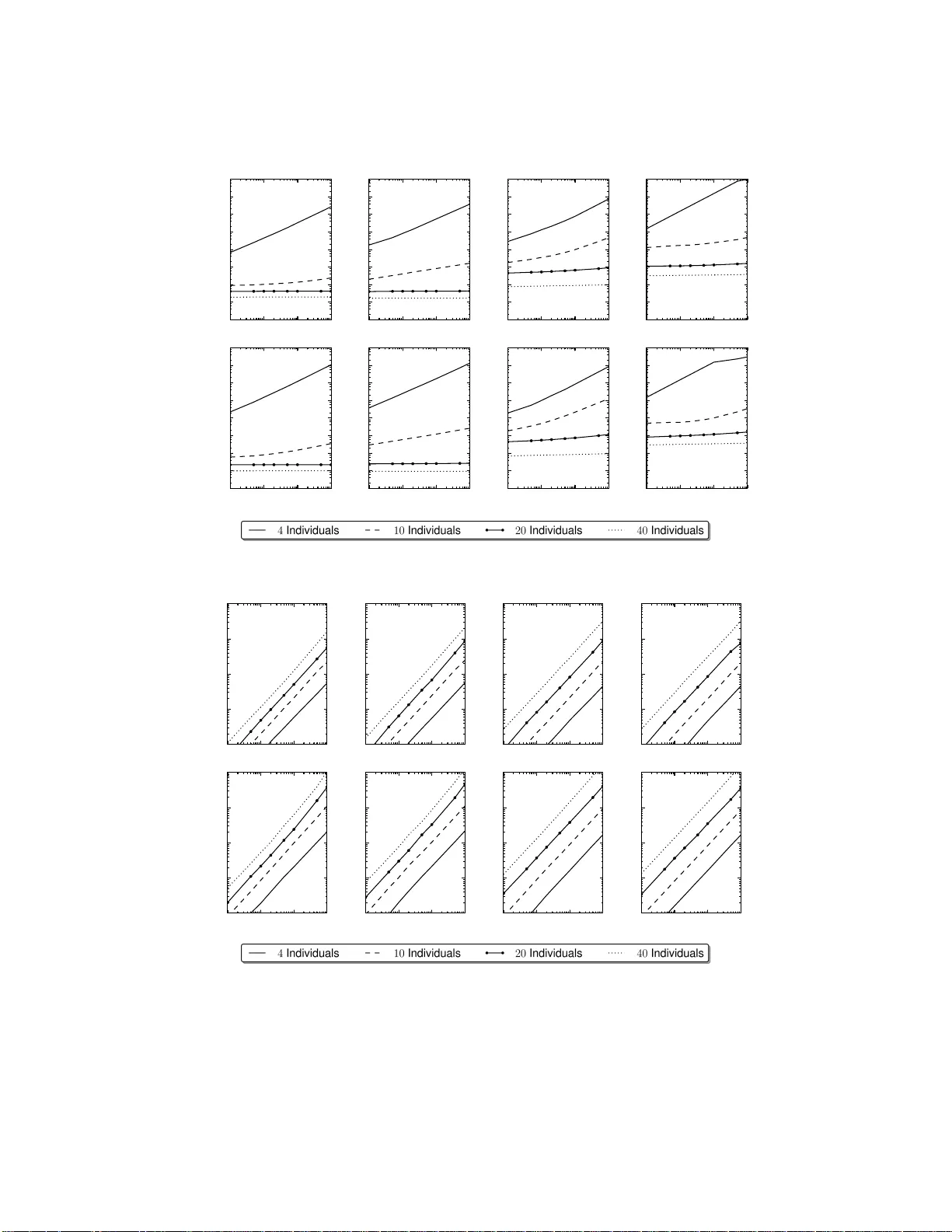
Efficien t Iden tification of Equiv alences in Dynamic Graphs and P edigree Structures Ho yt Ko epk e and Elizab eth Thompson ∗ August 9, 2021 Abstract W e prop ose a new framew ork for designing test and query funct ions for complex structures that v ary across a given parameter suc h as genetic marker p ositio n. The op erations we are inter- ested in include eq ualit y testing, set op eratio ns, isolati ng uniqu e states, duplication coun ting, or finding equiv alence classes under iden tifiabilit y constrain ts. A motiv ating applicati on is locating equiv alence class es in iden tity-b y-descent (IBD) graphs, g raph structures in p edigree analysis that change o ver genetic marker lo cation. The no des of these graphs are unlab eled and identified only by their connecting edges, a constraint easily han d led by our approach. The general framewo rk introduced is p o wer ful enough to b uild a range of testing funct ions for IBD graphs, dynamic p op- ulations, and other stru ct u res using a minimal set of op eratio ns. The theoretical and algorithmic prop erties of our approac h are analyzed a nd pro ved. Computational results on sev eral sim u latio ns demonstrate th e effectiveness of our ap p roac h. Keywords: Hash F unc tions, Algorithms, Data Structur es, P edigree Analysi s, Ident ity-b y-Desce n t Graphs ∗ Hoy t Ko epk e (E- mail: hoytak@stat. washington .edu ) is corresponding author and Graduate Studen t at Universit y of W ashingto n, Departmen t of Statistics. Elizabeth Thompson (E-mail: eathomp@u.washi ngton.edu ) is Professor at Unive rsity of W ashington, Department of Statistics, Seattle, W A 98195-4322. Thi s w ork was supp orted in part b y N IH gran t GM- 46255 . 1 1 In tro duc tio n In mo dern genetic analys es, w e hav e genetic marker data Y M on individuals av ailable at multiple genetic ma rk ers a cross the genome, and the para meters of g enetic marker mo dels, Γ M , are genera lly well es tablished. By co n tra st the mo dels Γ T underlying trait data ar e less clear. The goa l of genetic link age ana lyses is to lo cate DNA that affects the tra it relative to the known lo cations of the genetic marker map. This requires computatio n of the conditional probability P( Y T | Y M ; Γ ), where Γ is a joint mo del compr ising Γ M and Γ T and a sp ecification γ of the relative g enome lo cations of DNA underlying Y M and Y T . This probability will be required for m ultiple specific a tions o f the lo cation of DNA affecting the trait, and may b e required for mult iple v alues of tr ait parameter v alues Γ T and po ten tially for multiple tra it phenotypes on the same sets of related indiv idua ls. This key pr obabilit y is mos t easily co nsidered as P( Y T | Y M ; Γ ) = X Z P( Y T | Z ; γ , Γ ) P ( Z | Y M ; Γ M ) (1) where Z is an collectio n of laten t v ar iables insuring the conditional indep endence of Y M and Y T given Z . Class ically , the chosen laten t v a riables Z were the unobser v ed g enot y pes (types of the DNA) of the individuals of the p edigree str ucture [E lston a nd Stewart, 19 71, Lathr o p et a l., 19 84 ]. Mor e re c en tly a specifica tion of the inheritance of the DNA a t all relev ant lo cations has b een the preferred ch oice of Z [Lander and Green, 1 987, Lange a nd Sob el, 1991, Thompson, 1 994]. On large pedig rees, with data at multiple mar k e r lo cations, the probability in (1 ) ca nnot b e computed exactly , esp ecially if the data are spa rse on the pe dig ree structur es o r if these structur es a re c o mplex. Instead, rea lizations of Z from P( Z | Y M ; Γ M ) are obtained. A Monte Carlo es timate of P ( Y T | Y M ; Γ ) is the mean of the v alues o f P  Y T | S ( k ) ; γ , Γ T  ov er the N realiz e d  Z ( k ) : k = 1 , ..., N  . Several effective MCMC metho ds hav e b een develop ed to obtain thes e realizations [So b el and Lange, 1996, Thompson, 20 00 , T ong a nd Thompso n, 20 0 8 ]. In the context of mo dern informative marker data, an efficient c hoice of Z is the patter n of gene identit y by descen t (IBD), across the c hromos o me, among individuals observed for the tra it [Thompson, 2 011]. This defines a gra ph, the IBD g raph, which, at each locus , is analo gous to the descent gra ph of [Sob el a nd Lange, 199 6 ]. The edges of this gra ph are the obser ved individua ls, and the no des repr esen t IBD sharing at this ge nome lo cation amo ng the edg e s (individua ls ) co nnecting to that no de. The IBD graph is a deter ministic function of the inheritance sp ecification, and for mar ker genotypes Y M observed without err or, computation of the probability of these data for a giv en IBD graph is easy [Kr ugly ak et al., 1 996, Sobel and L a nge, 1996], Thus use o f the IBD gr aph led to gr eater efficiencies in o btaining MCMC realiz ations from P( Z | Y M ; Γ M ). How ever, it has b een less well appreciated that computation of P  Y T | Z ( k ) ; γ , Γ T  is also stra igh tfor w a rd using the IBD-g raph representation [Tho mps o n, 20 03, Thompso n and Heath, 1 9 99b]. Use of the IB D-graph has other immediate adv antages. They are generally slowly v arying acr o ss the ch romos o me, relativ e to moder n mark er densities, and may b e output from the MCMC in compact format, with o nly the c hang e p oints and c hanges sp ecified. Once the IBD gr aph is realized, the pedigree structure is no longer r equired in subsequent tra it-data analy s es, pr oviding greater data confiden tiality , and the same set of realiz e d IBD g raphs may b e used for multiple v alues o f ( γ , Γ T ) and even multiple different tra its obs erv ed on the same or different subs e ts of the indiv iduals [Thompson, 201 1 ]. When reduced to the subset of individuals observed for a trait, comp onen ts of an IBD-gra ph Z are genera lly small, so tha t for sing le-locus mode ls P( Y T | Z ; γ , Γ T ) is very easily computed, In fact, computation on the joint gra phs at several genome lo cations is also feasible, lea ding to metho ds for gene tic analysis under o ligogenic mo dels [Su a nd Thompso n, 20 12 ]. Finally , the IBD fra mew o rk has a key a dv antage in that it is not dep endent o n the source of the inferred IBD. 2 Using p opulation-base d metho ds, IBD may be inferred betw een any t wo individuals not known to b e related [Brown e t al., 2012, B ro wning and B ro wning, 20 10]. If these individuals a re p edi- gree founders or members of different p edigrees, such p opulation-based IBD may b e combined with pedig ree-based inferences of IBD to create merg ed IBD graphs , provided grea ter pow er and reso lution to trait analyse s [Gla zner a nd Thompso n, 20 12 ]. There is a no ther huge computational a dv a ntage p otent ially av ailable from the IBD-graph fra me- work. In an IBD graph, no des hav e an ident ity only through the edg es that connect them. Many different inh eritance patter ns S giv e rise to the same no de-unlab elled IBD graph on the subset o f trait- observed individuals. In an MCMC a nalysis, many different r ealizations of Z from P( Z | Y M ; Γ M ) may giv e the sa me IBD gra ph. Additionally , b ecause IB D-graphs are ge ne r ally slo wly v arying , a given realized IBD-graph ma y remain constant ov er several Mbp. Clearly , P( Y T | Z ; γ , Γ T ) should be computed once only for ea c h distinct Z . Reco gnition of when IBD-graphs are equal and o f the mar k er ranges ov er which they ar e equa l, is crucial to efficien t tr a it-data analyses. The softw are developed in this pap er p erforms this task efficiently , and ca n decrease the burden of the trait-data probability po rtion o f the LOD score estimation procedur e by up to t wo orders of magnitude in real studies [Marchani and Wijsman, 2 011]. The k ey o f our approa c h is to repr esen t the o b ject prop erties relev a nt to the testing by sets of representative hashes instead o f the o b jects themselves. H ashes permit muc h faster a lgorithms in many case s ; for example, testing whether tw o gra phs a re equal can b e done by checking whether tw o hashes are equal. Thes e hashe s ar e stro ng in the sense that in tersectio ns – unequal ob jects o r processe s mapping to identical hashes – a re so unlikely as to never o ccur in practice. F ur thermore, we introduce several prov a bly strong op erations on such hashes that allow accura te re ductions o f c o llections while maintaining sp ecified relationships betw een the hashes. Th us in our a pproach, desig ning test functions is equiv ale n t to designing comp osite hash functions ac cepting one or more input ob jects and retur ning a repres en tative hash. T esting equality over collections of input ob jects is then equiv alent to testing equality of the output hashes; set op erations over ob ject collections is equiv alent to set op erations ov er the hashes, and so o n. W e allow the ob jects in our fra mew o rk to change over a n indexing pa rameter. W e refer to this index as a marker , as it refer s to genetic mar k er po sition in our target application, but it could just as easily refer to time or any other indexing parameter . The p ow er of this framework is that the building blo c k oper ations pro cess along all the po ssible ma rk er v alues; the difficulties intro duce d by dyna mic data is abstra cted aw ay . The running example w e us e to illustrate this fra mew o r k a re identit y-by-descen t gr aphs, or IBD gr aphs [Sobel and La nge, 1996, Thompson and Heath, 1999a]. As an a bstracted structure, these graphs ha ve tw o interesting and distinctive prop erties. First, only the links are iden tifiable. In other words, equality on the gra ph structure is done str ic tly ov er links and the set of links attached to each node . Second, these gra phs change ov er ma rk er index ; o ne or more links may b e in different con- figurations b et ween distinct marker p oin ts. These graphs can b e a rbitrarily lar ge, with an ar bitr arily large r ange of mar k er v alues o ver which links can change lo cation, so brute for ce equa lit y testing at sp ecific ma rk er v a lues quickly b ecomes infeasible. The co mputational pro blems are exa cerbated when one wishes to work ov er la rge collectio ns of these, ma tc hing graph str uctures and lo oking for patterns. T o set up this exa mple, consider the g raph shown in Figure 1. Snapshots o f the graph G are shown at three marker v alues, m 1 < m 2 < m 3 . Now consider G ( m 1 ) in Figure 1a. As the no des and link s all hav e distinct lab els, it can b e represented by either listing the edges connec ted to each no de or the no des co nnected to each edg e as sho wn in T ables 1a and 1 b respec tively . Note that the structure of the graphs is uniquely describ e d by the sets in the right hand co lumn of either table. This allows us to test a g raph str uctur e without co nsidering la bels o n the no des but only on the edges , as we do for IBD graphs. F o r equality testing purp oses, this graph can b e repre s en ted exactly by first computing 3 (a) G ( m 1 ) (b) G ( m 2 ) (c) G ( m 3 ) Figure 1: An ex ample I BD graph G [ m ] w ith la b els on b oth edges and nod es. The nodes (n u m b ered) represent genetic sequences, while the edges (lettered) rep resent individu als. The graph changes slightly by marker v alue and is sho wn at marker val ues m 1 , m 2 , and m 3 . Note that under th e id entifiability constraints for I BD graphs, (a) and (c) are distinct d espite having the same skeletal stru ct ure. a hash over each connecting set, then ov er the set of resulting hashes; this is ess en tially what we do . No de Edges 1 A 2 A, B , E 3 B , C 4 C, D 5 D , E (a) Edge No des A 1 , 2 B 2 , 3 C 3 , 4 D 4 , 5 E 2 , 5 (b) No de Edges 1 A , E [ m 2 ,m 3 ) 2 A , B , E [ −∞ ,m 2 ) , D [ m 3 , ∞ ) 3 B , C , D [ m 2 ,m 3 ) 4 C , D [ −∞ ,m 2 ) , E [ m 3 , ∞ ) 5 D E (c) T able 1: (a, b) Two representations of the graph G ( m 1 ) from Figure 1a , by no de (a) and by edge (b) . (c) The same graph G at all marker p ositions with va lidity sets representing t h e differences in the graph at marker v alues m 1 < m 2 < m 3 . T o extend this to dynamic g raphs, we can a ssoc ia te v alidity informa tion with the comp onen ts of the gr aphs. Figure 1 shows G at marker lo cations m 1 < m 2 < m 3 , with slig h t but significant changes betw een them. Restricting ours elv e s to lo oking only at the by-nodes r epresen tation in T able 1a, a s the other is analog ous and this one is appropriate for IBD graphs, w e can des cribe G by T able 1c. This pro duces a collection of s ets that v a ries by marker v alue; this example will be explored further throughout this pap er since working with dynamic colle ctions such as this one is the target application of our fr amew o rk. The pap er is s tructured as follows. In the next sectio n we br iefly describ e so me related work, mostly inv olving innov ative us es of non- in ters ecting has hes. In section 3, w e formalize what we mean by a hash and describ e a set of basic functions over them with theoretic gua r an tees. Then, in section 4, we extend our theory of has hes to include mar ked hashes by desc r ibing marker v alidity sets and the data structures we use to make marker op erations efficient. Section 5 details M-Sets, our mos t significa n t contribution, along with av aila ble op erations. Finally , in section 6, we illustrate the flexibility o f our approach with several ex amples. 4 2 Related W ork Hash functions and r elated algorithms hav e seen numerous a pplications. The unifying principle is that a short “digest” is calculated ov er the messa ge o r data in such a wa y that changes in the data are r e flected, with sufficiently high proba bilit y , in the digest. Arguably the mo st widespr e ad use of hash-like algor ithms ar e with chec k- sums and cyclic redun- dancy chec ks (CRCs) [Maxino and Ko opman, 200 9 , Nak a ssis, 1988, Peterson and Brown ]. These are used to v erify data integrity in everything fro m file systems to Internet transmiss ion proto cols, and are usually 32 or 64 bit and desig ned to detect random erro rs. The chec ksum is stored o r trans mitted along with the da ta. When the data is rea d o r received, the chec ksum is r ecalculated; if it do esn’t match up with the origina l chec ksum, it is a ssumed tha t an er ror o ccurred. In cryptog raph y , hashes , or “messag e digests”, give a signature of a message without revealing any information ab out the message itself [Sc hneier, 20 07]. F or exa mple, it is co mmon to store passwords in terms of a ha sh; it is imp ossible to deduce what the pass w o rd is from the hash, but easy to check for a pa ssw ord ma tch. Muc h like a checksum, it is a lso used to ensur e messag e s have not b een tampe red with; as it is ex tremely difficult to pro duce different messa ges tha t hav e the same digest. It is this prop ert y that we utilize in o ur appro ac h. Representing data b y a hash is also commo n. Ha s h table s , a da ta structure for fa s t lo okup of ob jects given a key , works by first creating a hash of the key and using that hash to index a lo cation in a n array in which to store the o b ject [Cor men et al., 2001]. The hashes used in such tables are usually weak, as calculating the hash is a significant e fficiency b ottleneck and the siz e of the loo kup array determines how many bits of the hash a re a ctually needed – usua lly not all. Collisions – distinct op erations ma pping to the same hash – ma y b e co mmon, so further equality testing is p erformed to ensure the indexing keys match. Thus such hash ta bles tend to b e re lativ e ly complicated s tr uctures. Stronger ha sh functions us ually pro duce hashes with 128 or more bits, large eno ugh that the pro b- ability o f collisions is so low as to never o ccur in practice. Databas e applications often use such hashes to index lar ge files, as the no n-existence of co llisions g r eatly simplifies pr oces s ing [Silb erschatz et al., 1997]. Similarly , ne tw ork applications often use such hashes to cache files – files having the s ame hash do not need to b e retr ansmitted [B a rish and Obra czk e, 2000, Karg er et al., 1999, W a ng, 19 99]. Often cryptogr a phic has h functions a re use d for this purp ose; while slow e r, they ar e computed without using net work reso urces, so calculating them is no t the main efficiency b ottleneck. F ur thermore, they a r e strong enough that has h equality essentially guara ntees ob ject equality . Our application extends several of these ideas, most no tably the las t one. W e use strong hash functions to r epresent arbitrary ob jects in our framework, a ssuming equa lities among hashes are trustw or th y . Ho wever, our fra mew o rk extends pr evious work in that it relies heavily on s ev er al op er- ations over hash v alues to reduce the information pr esen t in co llections down to a single ha s h that is inv ariant to sp ecified as p ects of a pro cess. W e pres en t s ev er al theore ms that guara n tee the summary hash is also strong. This allows us to reduce co mputatio ns that would be c o mplex when p erformed ov er the o riginal da ta str uctures to simple o pera tio ns ov er hashes while e ns uring that the results a re accurate. 3 Hashes F or our purp ose, the hash function H ash maps from an arbitr ary ob ject or other ha sh to an integer in the set H N = { 0 , 1 , ..., N − 1 } in a wa y that satisfies several pro perties. Fir st, s uc h a function must be one-way ; i.e. no infor ma tion a b out the original ob ject ca n be rea dily deduced from the hash (e.g. “ab cdef ” a nd “Ab cdef ” ma p to unrelated hashes ). In other w ords, having access to the output of 5 such a hash function is e q uiv alent to having a c c ess o nly to an or acle function that returns true if a query ob ject is equal to the original a nd ob ject and, with hig h probability , false otherwise [Canetti, 1997, Canetti et al., 199 8 ]. Under these re quiremen ts, Hash can b e seen as a discrete, uniformly distributed ra ndom v a riable mapping from the even t space – arbitra r y ob jects or other hashes, etc. – to H N . This form allows us to assume Ha sh ( ω ) has a uniform distribution o n H N for an arbitr a ry ob ject ω , a for m useful for the pro ofs we give later on. F urthermo re, the “ora c le” prop erty implies that the distributions of t wo hashes ar e indep enden t if the indexing ob jects are distinct. Second, Hash must b e strong, i.e. collisions – unequal ob jects mapping to the same hash – are extremely impro bable. F orma lly , Definition 3.1 (Strong Hash F unction.) . A hash function Hash mapping fro m an arbitra ry ob ject ω to a an integer in H N = { 0 , 1 , ..., N − 1 } is consider e d st r ong if, for h 1 = Hash ( ω 1 ) and h 2 = Hash ( ω 2 ), P( h 1 = h 2 ) =  1 ω 1 = ω 2 1 / N ω 1 6 = ω 2 (2) The idea is to set N larg e enough (in our ca s e ar ound 10 38 ) that the pro babilit y of t wo unequal ob jects yielding the same has h is so lo w as to nev er o ccur in practice. How ever, in lig h t of the fact that collisions can theoretically o ccur with nonzero pr obabilit y , we deno te inequality as ≁ instead of 6 =; sp ecifically , if h 1 = Has h ( ω 1 ) ≁ Hash ( ω 2 ) = h 2 , then P( h 1 = h 2 ) = 1 / N . W e may assume the ex istence of such a hash function, denoted he r e as H ash , which maps any po ssible input – str ings, num b e r s, o ther ha s hes – to a ha s h that sa tisfies definition 3 .1. This assumption is reasona ble, a s significant rese arc h in cryptogra ph y ha s gone towards developing hash functions that not only satisfy definition 3.1, but also preven t adversaries with large amounts of computing p o wer against deducing an y information about the orig ina l ob ject [Goldreich, 2 001, Schneier, 200 7 ]. These hash functions are widely av aila ble a nd have op en s p ecifications; we use a tw ea ked version of the well known md5 ha sh function a s o utlined in app endix App endix A. 3.1 Hash Op erations Based o n the exis tence of a hash function Hash , and simple o pera tio ns on integers in H N , we prop ose t wo basic op erations to combin e a nd mo dify hashes. The first is a w ay to summarize an unordered collection of hashes by r educing it to a single ha sh that is sens itiv e to changes in the hash v a lue of any key in the orig inal co llection. The se c ond, to b e used in nested function comp ositions, is a way to scra mble a reduced has h v alue so that it lo cks inv aria nce prop erties present ea r lier in the function comp osition. In this section, we formally describ e these op erations , which will later b e g eneralized to bo th marked hashes and then to co llections of mar k e d has hes . 3.1.1 T ransformations W e now m ust forma lize what w e mean by a transfor mation in the testing function context. In o ur terminology , a tr ansformation always applies to the inputs of a tes ting function and is done without regar d to the hash v a lues themselves. F o r ex a mple, any reor dering of the input v alues is a v alid transformatio n, but a ppending a precomputed string to the lab el of an input ob ject to ca use its has h to b e the s pecial null-hash – all zero s – is not (Note, how ever, that forming the null-hash in this wa y is near- imp ossible in prac tice). F ormally , Definition 3.2 (T ransfor mation Class es) . A transfor ma tion class for a testing function T s atisfies: 6 T1. Every T ∈ T ca n b e expr essed as a transforma tion of the non-hash input ob jects. T2. No T ∈ T ta k es a ccoun t of the sp ecific hash v alue s pro duced by these o b jects. Given these restrictions on transfor mation cla sses, we can now for mally define what w e mean by inv arianc e . Definition 3.3 (Inv a riance a nd Distinguishing) . A function f : H n N 7→ H n accepting a set o f inputs h = ( h 1 , h 2 , ..., h n ) is invariant under a class of tra nsformations T if f ( T h ) = f ( h ) for a ll T ∈ T and for all h ∈ H N . Likewise, f distinguishes T if, for T 1 , T 2 ∈ T , f ( T 1 h ) ≁ f ( T 2 h ) ≁ f ( h ) unless T 1 h = h , T 2 h = h or T 1 h = T 2 h . In o ther words, the output hashes change under distinguishing tr ansformations and are co nstan t under inv ar ian t transfo r mations. With these for mal definitions, we ar e now prepared to define atomic op erations that have sp ecific and pr o v able inv aria nce prop erties. 3.1.2 The Null Hash W e chose one v alue in our ha sh set, sp ecifically 0, to repr esen t a Nul l hash. This ha sh v alue, deno ted as ∅ , is used to re pr esen t the a bsence of a n input o b ject. It most commonly represents the hash of a n ob ject tha t is outside its mar ker v alidity set; this will be detailed mor e in section 4. As such, it has sp ecial pr oper ties with the hash o peratio ns outlined in the next s ection. 3.2 Hash Op eration Prop erties W e here pro p ose tw o ba sic op erations, Reduce and Rehash . The firs t reduces a collection of n hashes, h 1 , h 2 , ..., h n for n = 1 , 2 , ... , down to a single hash, while the second rehashes a single input hash to pr ev ent inv aria nce prop erties from propaga ting fur ther through a function comp osition. The key asp ects of these op erations are what tr a nsformations over the inputs they ar e inv a r ian t under ; we describ e these next. W e follow this with a brief discussion o f the implications of these re s ults, b efore detailing the construction of such functions in section 3.3. Definition 3.4 ( Reduce ) . F or the Reduce function, with h 0 = Reduce ( h 1 , ..., h n ), we have the following pr o perties: RD1. Invarianc e Under the nul l hash ∅ . The output hash h 0 is inv ariant under input of the null hash ∅ . Sp ecifically , Reduce ( h 1 , ∅ ) = Reduce ( h 1 ) Reduce ( ∅ ) = ∅ RD2. Invarianc e Under Single Mapping . The output hash h 0 equals the input hash h 1 if n = 1. Spec ific a lly , Reduce ( h 1 ) = h 1 RD3. Existenc e of a ne gating hash . There exists a neg ating hash, here la beled − h 1 , that cancels the effect of a n input hash in the sense that Reduce ( h 1 , − h 1 ) = Reduce ( ∅ ) = ∅ 7 RD4. Or der Invarianc e . T he output hash h 0 is inv aria n t under different order ings of the input. Sp ecif- ically , Reduce ( h 1 , h 2 ) = Reduce ( h 2 , h 1 ) . RD5. Invarianc e U n der Comp osition. The output has h h 0 is in v ariant under nested comp ositions o f Reduce . Sp ecifically , Reduce ( h 1 , h 2 , h 3 ) = Reduce ( h 1 , Reduce ( h 2 , h 3 )) = Reduce ( Reduce ( h 1 , h 2 ) , h 3 ) RD6. Str ength . The Reduce function distinguishes all other tra nsformations in the sense of definition 3.3 ( e.g . an input v alue is dro pped or changed). Two remarks ar e in o rder. First, prop erty RD5 allows us to expand a ll nestings of Reduce to a single function of ha shes that ar e not the output of Reduce op erations. F o r e x ample, Reduce ( h 1 , Reduce ( h 2 , Reduce ( h 3 , h 4 ))) = Reduce ( h 1 , h 2 , h 3 , h 4 ) The implica tion is that when we have a collection o f input ha shes h 1 , h 2 , ..., h n , which may or may no t hav e come from a reduction themselves, we can wr ite their reduction out a s a single r e duction; i.e. Reduce ( h 1 , h 2 , ..., h n ) = Reduce ( h ′ 1 , h ′ 2 , ..., h ′ n ′ ) for some hashes h ′ 1 , h ′ 2 , ..., h ′ n ′ that ar e not the res ult of Reduce . Second, prop erty RD3 allows us to remov e elements fr om a re ductio n o nce they ar e a dded, making the reduced hash in v ariant under c ha nges in wha tev er pro cess pro duced the ca nceled hash. This prop ert y b ecomes esp ecially useful later o n when working with interv a ls; the o utput ha sh v aries as a function of a marker v alue, and a hash h v a lid on an interv a l [ a, b ) of that ma rk er can b e added once at a and removed at b , with the net r esult b eing that the output has h is only s ensitiv e to h on [ a, b ). Definition 3.5 ( Rehash ) . F or the Rehash function, we have only tw o pro p erties, which w e list here. RH1. Invarianc e Under t he nu l l hash ∅ .The output hash h 0 is inv ar ia n t under input of the null hash ∅ . Sp ecifically , Rehash ( ∅ ) = ∅ RH2. Str ength . The Rehash function is strong in the sense o f definition 3.1, in which the ob ject space is restric ted to hash keys. The purp ose o f the Rehash function is to freeze in v ariance pa tterns from pr opagating through m ultiple comp ositions. Retur ning to the example IBD graph in Fig ure 1, c o nsider the testing function shown in Figure 2 . The function resulting fro m chaining Reduce and Rehash together as shown is inv ariant under changes in the no de lab els or or derings of the edg es within each no de, but is sensitive to any structural change in the gr aph. This can be prov ed by decompos ing the nested Reduce functions into a single function of the first group; a ll the inv a rian t relationships of this single function are pres en t in the o riginal. How e ver, the final reduce cannot b e decomp osed this wa y on account of the Rehash functions. 8 Figure 2: P art of a comp osite function fo r testing equality , ignoring no de labels, of the graph G ( m 1 ) in Figure 1 . The part of the function for the first 3 n odes are sho wn. F or eac h no de, the lab els on the connected edges are reduced into one hash, and then t he hashes rep resenting the nod es are red uced to a final hash which represents th e graph. This final hash is inv arian t under changes in the no de lab els or orderings of the edges within each no de, but is sensitive to any structu ral c hange in the graph. 3.3 F unction Construction and Implemen tation W e now e s tablish that functions Reduce and Rehash satisfying the appro priate prop erties exist. Along with this comes a requirement on N , namely that it is prime ; this is required to preserve the strength of the Reduce function under multiple reductions of the same ha sh key . 3.3.1 Basic Op erations Before presenting the Reduce and Rehash functions, we firs t prese nt tw o lemmas fro m elementary nu mber theor y . Thes e lemmas provide the theoretical basis of the Reduce function. Lemma 3 . 6. L et N b e prime, and let ⊕ and ⊗ denote addition and mu ltipli c ation mo dulo N , r esp e c- tively. Supp ose a, b ∈ H N . Then the following e quivalenc es hold mo dulo N : ( a ⊗ b ) ⊕ b ≡ ( a ⊕ 1) ⊗ b (3) − ( a ⊕ b ) ≡ ( − a ⊕ − b ) − ( a ⊗ b ) ≡ ( − a ⊗ b ) ≡ ( a ⊗ − b ) Pr o of. The in tegers mo dulo N forms an algebraic field with distributivity of multiplication over ad- dition, so ((3)) is trivia lly sa tisfied. F urthermor e, − h ≡ ( − 1) ⊗ h ≡ ( N − 1) ⊗ h mo d N Thu s − ( a ⊕ b ) mo d N ≡ ( − a ⊕ − b ) mo d N . Similarly , m ultiplication is commutativ e, so − ( a ⊗ b ) ≡ (( − 1) ⊗ a ) ⊗ b ≡ ( − a ⊗ b ) mo d N ≡ ( a ⊗ (( − 1) ⊗ b )) ≡ ( a ⊗ − b ) mo d N The lemma is pr o ved. 9 Lemma 3.7. L et N b e prime, and let X and Y b e indep endent r andom variables with distribution Un ( H N ) , i.e. uniform over H N , and let r b e any n u mb er in H N . Then C ⊕ X ∼ Un ( H N ) (4) − X mod N ≡ N − X ∼ Un ( H N ) (5) X ⊕ Y ∼ Un ( H N ) (6) r ⊗ X ∼ Un ( H N ) , (7) i.e. the ab ove ar e al l uniformly distribute d on H N . Pr o of. F o r (4), note that addition mo dulo a constant is a o ne-to-one a uto morphic ma p on the has h space, thus ev e ry mapp ed n um b er is equally lik ely . (5) is similarly prov e d. T o prove (6), no te tha t Y can b e s een a s a similar rando m mapping ; how ever, every p ossible mapping pro duces the same distribution ov er H N , so X ⊕ Y has the same distribution as X ⊕ Y | Y , which, by (4) is uniform on H N . F or (7), reca ll from num b er theory that r has an inv erse mo d N if and only if r a nd n are copr ime, i.e. gc a( r, n ) = 1. Thus if N is prime, each r in H N also indexes a one- to-one automor phic map under r ⊗ X , and the result immediately follows. 3.3.2 Reduce W e a re now ready to tackle Reduce ; if N is prime, then addition mo dulo N satisfies all the required prop erties. This op eration is simila r to pa r t of the Fletcher chec ksum algor ithm, which uses a ddition mo dulo a 16 -bit pr ime for the reaso ns outlined in lemma 3.7. Theorem 3.8 (The Reduce F unction.) . Supp ose N is prime. Then the function f : H n N 7→ H N define d by f ( h 1 , h 2 , ..., h n ) = h 1 + h 2 + ... + h n mo d N = h 1 ⊕ h 2 ⊕ ... ⊕ h n , wher e ⊕ denotes addition mo dulo N , satisfies pr op erties RD1-RD6. Pr o of. Addition modulo N , with N pr ime, forms an a lg ebraic g roup, s o pr operties RD1, RD2, RD4 and RD5 are triv ially s atisfied. RD3 is satisfied w ith − h 1 ≡ N − h 1 mo d N . T o prove RD6, it is sufficient to verify equatio n (2) in definitio n (T1). Let h 0 = Reduce ( h 1 , h 2 , ..., h n ), and let k 0 = Reduce ( k 1 , k 2 , ..., k m ). Without loss of generality , by the previous prop erties, let the sequences b e a s follows: 1. No ha sh in either sequence is the neg ativ e of another hash in that sequence. 2. n ≥ m ; if not, swap sequences. 3. There exists an index q ∈ { 1 , 2 , ..., m } such that h i = k i for i ≤ q a nd h i / ∈ { k q +1 , ..., k m } for i = q + 1 , ..., m . 4. h 1 = k 1 = ∅ (so q ≥ 1 , to make b o okk eeping ea sier). Now supp ose the tw o sequenc e s ar e iden tica l, so n = m = q . Then h 0 = k 0 and we are done; this satisfies the first pa r t of equation (2). Otherwise, we ca n use lemma 3.6 to re presen t h 0 and k 0 as h 0 = Q ⊕ ( α 1 ⊗ H 1 ) ⊕ ( α 2 ⊗ H 2 ) ⊕ · · · ⊕ ( α n ′ ⊗ H n ′ ) k 0 = Q ⊕ ( β 1 ⊗ K 1 ) ⊕ ( β 2 ⊗ K 2 ) ⊕ · · · ⊕ ( β m ′ ⊗ K m ′ ) 10 where Q = Reduce ( h 1 , h 2 , ..., h q ) and H 1 , H 2 , ..., H n ′ , K 1 , K 2 , ..., K m ′ are all indep enden t and α 1 , ..., α n ′ , β 1 , ..., β m ′ denote the multiplicit y o f each hash. Now it re mains to show that P( h 0 ≡ k 0 mo d N ) = 1 / N . Now P( h 0 ≡ k 0 mo d N ) = P( h 0 ⊕ − k 0 ≡ 0) and, using lemma 3.6 to distribute the min us signs and eliminate the Q s, h 0 ⊕ − k 0 = ( α 1 ⊗ H 1 ) ⊕ ( α 2 ⊗ H 2 ) ⊕ · · · ⊕ ( α n ′ ⊗ H n ′ ) ⊕ ( β 1 ⊗ − K 1 ) ⊕ ( β 2 ⊗ − K 2 ) ⊕ · · · ⊕ ( β m ′ ⊗ − K m ′ ) . How ever, applying lemma 3.7 inductiv ely gives that the distribution of the a b ov e is uniform over H N . Thu s P( h 0 = k 0 ) = 1 / N . 3.3.3 Rehash Now on to Rehash , which is far simpler a s it relies mainly o n the prop erty of the ha sh function b eing strong. The o nly ex tr a work is to ensure that the null hash is preser ved. Theorem 3.9 ( Rehash ) . The funct ion Rehash : H N 7→ H N define d by Rehash ( h ) = Reduce ( Hash ( h ) , − H ash ( ∅ )) , satisfies pr op erties (RH1)-(RH2) while distinguishing al l other tr ansformations. Pr o of. F o llows trivia lly from the prop erties of Reduce a nd the assumption that Hash is strong and one-wa y . In this section, we hav e presen ted the fundamen tal building blocks reg arding hashes. W e now augment these hash v alues with v alidity informatio n that v aries as a function of a particular parameter , here called a ma rk er v alue . 4 Hashes and Keys W e define a key as a hash v alue as socia ted w ith a set of interv als within which that hash, or the o b ject it refer s to, is v a lid. A key may re pr esen t an ob ject in the data s tructure we wish to des ign a testing function for , e.g. an edge in a g raph tha t is present only for ce r tain marker v alues, or it may repr esen t the result o f a pro cess or sub-pro cess. At the marker v alues for which this key is not v alid, we assume its ha sh is equal to ∅ . T o denote the hash v alue o f any key a t a c e rtain v alue p of the para meter space, we use brack ets – e.g. h [ p ]. The set on which the hash v alue of a key is v alid, which we call a marker validity set o r just validi ty set , is a seq uence of sorted, disjoint interv als of the form [ a i , b i ) ⊆ [ −∞ , ∞ ). A marke d o b ject is valid in each o f these in terv a ls and invalid elsewhere . Saying s omething is unmarke d is equiv alent – for bo okkeeping reasons – to s a ying that it is always v alid, i.e. on the interv al [ −∞ , ∞ ). 5 Mark ed S ets The M-Set, a c on ta iner of mar k ed keys, is the most p ow erful comp onent of our fra mew o rk. It can b e thought o f a s a collection of marked ob jects, stored as representativ e k e y s, that p ermits easy acces s to useful informatio n ab out the co llection. The idea is that one can express many algorithmica lly 11 complicated pro cessing tasks inv olving dynamic data a s simple ope r ations on and betw e e n M- Set ob jects. Efficient op erations o n an M- Set include querying, inser tion, deletion, testing collection equality at sp ecific mar k er v alues or over the whole collection, union and intersection, and ex tracting the collec tion of keys v alid at sp ecific marker v alues . 5.1 Op erations Av ailable M-Set oper ations fall into five categ ories: element op er ations lik e insertion, q uerying, or mo difying an element’s v alidity set; hash and test ing op er ations like deter mining whether tw o M- Sets ar e identical at marker m ; set op er ations such as union and in tersection; valid ity set op er ations such as extracting a ll hashes v alid at a certain point; and summarizing op er ations which pro duce representative hashes from one or more M-Sets. Of thes e , op erations in the first four c ategories ar e easily expla ined; we present them in the next sections. The summarizing op eration, whic h is key to the p o wer of our fr a mew o rk, is pres en ted in sec tio n 5.2. A list o f all these functions is given in s ection B.2; the most powerful ones we descr ib e now. 5.2 Summarizing Op erations: ReduceMS et and Summarize The natural generaliz ation of Reduce to M-Set ob jects, ReduceMSet , r eturns an M-Set containing the reductio n of every key in the se t. F orma lly , for M-Sets T 0 and T 1 , supp ose T 0 = ReduceMSet ( T 1 ). Then, for e a c h marker v alue m , ther e is exactly o ne key in T 0 v alid a t m , with that ha sh b eing the Reduce of every key in T 1 v alid at m . The M-Set is the appr opriate output o f this function, as the resulting hash v alue v ar ies arbitr a rily by marker v alue a nd thu s c annot b e ex pressed as a single k ey . Because such an M-Set has exa ctly o ne ha sh (pos sibly ∅ ) v a lid at each mar k er v a lue, we use the same brack et nota tio n as keys to refer to that ha sh v alue, e.g. T [ m ]. Lo oking up the reduced has h o f the M-Set at sp ecific mar k e r lo cations – HashA tMarker – is efficient to do witho ut r educing the en tire set. The main use for ReduceMSet is thus to crea te a lo okup o f the p ossible v alues of Reduce in that set and when they are v a lid a s r e presen ted by the v alidity sets of the r esulting k eys. This can, for example, b e used to determine the se t on which a dynamic collectio n is equal to a given collection. Just as ReduceMSet summar izes the information in a colle c tion of k eys b y a single M-Se t, so Summarize reduces the infor mation from one or more distinct collections of M-Sets down to a sing le M-Set ov e r which computations can accur ately and efficiently b e do ne. Cha nges in any individual collection, as well as which collections ar e included, are alwa ys reflected in the summarizing M-Set unless they fall under one of the inv aria n t pr o perties (e.g. ∅ do es not affect the outco me). As such, Summ arize pro duces an M-Set T in which one ha s h is v alid a t e a c h given marker p osition m . F or T = S ummarize ( T 1 , T 2 , ..., T n ), the hash key v alid at m , T [ m ], is equa l to T [ m ] = Reduce (  Rehash ( h ) : h = ReduceMSet ( T i ) at m, for i = 1 , 2 , ..., n  ) Given our implemen tation o f ReduceMSet , descr ibed in the next section, the Summarize op eration is very efficient a nd a central building- blo ck in our framework. The s ummarizing o pera tio n is useful in that it allows us to efficiently test equality of collectio ns of M-Sets using the op erations designed for hashes. F or example, supp ose we have tw o summar y M-Sets, T = Summarize ( T 1 , T 2 , ..., T n ) and U = Summarize ( U 1 , U 2 , ..., U n ). Giv en T [ p ], the marker v a lidit y set of the corresp onding key in U , if any , gives the set in which the collectio n of T i ’s at p is equal to the collection o f U i ’s. Likewise, MarkerU nion ov er all o b jects in the intersection of T and U gives the lo cations a t which the tw o collections are equa l. 12 Figure 3: A skip- list with 3 levels and 10 v alues. 5.3 Implemen tation Int ernally , an M-Set is a combination of a hash table to s tore the hashes and a s kip-list-t yp e structure that handles the bo okkeeping op erations dealing with v a lidity sets. This latter structure efficiently tracks the Reduce at each mar k er v alue of all keys pres e n t in the structure; this is key to making op erations like equality testing a nd summar izing e fficie n t. 5.3.1 Skip Lists for Mark ers T o introduce the augmented s kip-list for the Reduce lookup, we first describ e a simpler version for ho lding marker information. In a skip-list, the v alues are stored in a single o rdered linked list; this a llo ws for easy insertion a nd deletion, but by itself do es not p ermit efficient ac cess. T o access them e fficie n tly , there are additional levels of incr easingly spar se linked lis ts, ea c h a subset of the previous, with each no de p oin ting forward and po in ting down to the cor respo nding no de in the low er level. When a new v alue is inserted in the skip- list – in our case a v alidity interv a l – it also adds corres p onding no des in the L levels ab ov e it, where L ∼ Geom etric ( p ). The geo metr ic distribution of the no de “heights” mea ns the exp ected size of level L is np L . Overall, the exp ected times for querying , insertion, o r deletio n is O (log n ) [Devroy e, 1992, Kir sc he nho fer and P r odinger, 19 94, Papadakis et al., 1992]. An e x ample skip-list is shown in Figure 3. In this skip-list, ea ch mar k er loca tion, denoted by k m 1 , ..., k m n , has corr esponding no des in 0 to 3 levels ab o ve it. The interv al starting v alues are stored in the no des at ea c h level. Querying is done a s follows. Star t at the first no de in the highest level, which is alwa ys at −∞ . If a forward no de exists a nd its v alue is less than o r equal to the q uery v alue, mov e forward; otherwise, mov e down. Rep eat this until you’re on the low er level a nd cannot adv a nc e any far ther; if this interv al contains the q uery v a lue, tha t mar k er v a lue is v alid, otherwise it is not. Finding lo cations for insertion and deletion are a nalogous. 5.3.2 In ternal Re duce Lo okup W e now present the da ta s tructure that comprise s the seco nd comp onen t of a n M-Set. This str uc tur e allows for calculating Reduce , for a given marker v alue, ov er all compo ne nts of the entire hash collection in logar ithmic time while still allowing loga rithmic time insertion a nd deletion. With this 13 Figure 4: The left part of th e table in Figure 3 adapted to b e an M-Set hash lookup struct ure holding hash information in the skip - list no des. H ash keys, v alid for certain marker in terv als, are show n in the b ottom, while th e information stored in each no de is shown b elo w t he n ode lab el. structure, we can a lso ca lculate Reduce ov er a ll v a lidit y s et interv als v alues in time linear in the nu mber of distinct v alidity interv a l endp o in ts, pr oducing a new M-Set of keys with non-intersecting v alidity s ets represe nting the differe nt v alues of Reduce at v arious marker interv als. Thes e algor ithmic bo unds and the asso ciated algor ithms will b e for malized b elow. The str uc tur e we pro p ose is an a ugmen ted skip-list. The leaf and no de v a lues present in the tree corres p ond to the int erv al endpo in ts in the v alidity interv a ls of any key pr esen t, i.e. the mar k er v alues where the v a lidit y of a n y key changes. This list is a ugmen ted to hold a hash key in each leaf and each no de. The main idea for the lea f ha shes is to track Reduce over all v a lid keys as a function of mar k er v alue m . Stepping thro ugh the lea ves, starting with the has h v alue in the first leaf and up dating it with the leaf hash using Reduce , yields Reduce over a ll v alid hashes at each marker v alue. This is done by including a hash at the b eginning o f each of its v alidity interv a l and the nega tive of that hash at the end of a v a lidit y in terv al. Thus has h v alues a re added a nd removed fro m the o verall reduced hash to maintain the v a lue of Reduce at each marker v alue. This a llows us, additionally , to calcula te the M-Set pro duced by ReduceMSet efficiently by simply stepping thro ugh the leav es. Figure 4 shows an example augmented sk ip-list, the structure of which is taken fr om the rig h t half 14 of the example skip- list in Figure 3. The leav es hold has h v a lue s tha t are the reductio n of has h v alues and/or nega tive ha s h v alues. A t a given marker v alue, the v alue of Reduce ov er all previo us lea ves is the v a lue of Reduce ov er all curr en tly v alid keys. F or example, lo oking at the first thr ee leaves, Reduce ( k m 6 , k m 7 , k m 8 ) = Reduce ( Reduce ( h 1 , h 2 ) , Reduce ( − h 1 , h 3 ) , Reduce ( − h 3 )) = Reduce ( h 1 , h 2 , − h 1 , h 3 , − h 3 ) = Reduce ( h 2 ) F ormally , we maintain the following prop erty: Prop ert y 5.1 (M-Set Mar k er Sk ip-List Lea f Hashes) . F or a given M-Set T with s kip-list S , let L [ m ] = { h : m = ℓ for some [ ℓ, u ) in the validity set of h } U [ m ] = { h : m = u for some [ ℓ, u ) in the validity set of h } Then for al l le aves in S , define the hash value r 0 [ m ] at t hat le af to b e r 0 [ m ] = Reduce ( { h : h ∈ L [ m ] } ∪ {− h : h ∈ U [ m ] } ) Thu s we can for mally state the ab o ve. Theorem 5. 2. L et T b e an M-Set with c orr esp onding le af no des r 0 [ · ] . L et R [ m ] = Reduce ( { r 0 [ m ′ ] : m ′ ≤ m } ) . Then R [ m ] = Reduce ( { h [ m ] : h ∈ T and h is valid at m } ) , Equivalently, R [ m ] = Reduce ( { h [ m ] : h ∈ T } ) , Pr o of. On the marker interv als where a has h key is v alid, its has h is included in R [ m ] exa c tly one time more than its inv erse is included, and it is included exactly the same n umber of times as its inv er se at all other v a lues. F rom prop erty RD3, the summary Reduce hash at m depends on a ha s h key if and only if that hash key it is v alid a t m . The equiv alent fo r m ula for R [ m ] follows immediately from the fact that h [ m ] = ∅ if h is not v a lid at m ; which do es not change R [ m ]. As men tioned, the Reduce of all leaf hash v alues whose asso ciated marker v alue is less than or equal to the giv en mar k e r v alue m is eq ual to the Reduce of all the keys in the M-Set v alid at m . How ever, storing the hashes in this w ay at the leaves is not e no ugh to efficie ntly compute Reduce quickly over the full has h table a t a given mar k er v a lue m , a s it would requir e vis iting every change- po in t pr e sen t that is less than m . One mig h t sug gest s toring R [ m ], the full v a lue of Reduce , at the leav es instead of just r 0 [ m ], but then inser tion and deletion would re q uire time linea r in the num b er of mar k e r p oin ts pr esen t in v a lid interv als, and this ca n b e ar bitrarily lar ge. Our s olution is to stor e a has h v alue summarizing blo c k s of r 0 [ m ] in the no des at higher levels in the skip-list structure. The idea is that the hash v a lue stored in the nodes is the reduction of all leav es under it. The pr esence of these hash v alues at the no des allows us to construct logar ithmic time alg orithms for querying , inse r tion and deletio n. The idea is that we can include the reduction o f large blo cks of no des with a single o p eration as we tr a vel down the skip-list. F ormally , at the no des, these hash v alues maintain the following pro p erty: 15 Algorithm 1 : HashA tMarkerV alue Input : M-Set T and marker v alue m . Output : Hash V alue h , the Reduce ov er all hash ob jects in T at m . h ← 0 n ← Fir st no de o f highest level of skip-list of T while not at destination le af do if nex t n o de n ′ has marker value ≤ m then h ← Reduce ( h, hash at no de n ) n ← n ′ else n ← no de b elow n return h Prop ert y 5.3 (M-Set Skip-Lis t No de Pro perty) . L et r b [ m ] b e a hash value at marker value m in the b th level of the skip-list with b ≥ 1 ( b = 0 is t he le af level). L et m ′ b e the sm al lest marker value lar ger than m , p ossibly ∞ , such t ha t ther e exists a no de at level b with marker value m ′ . Then r b [ m ] = Reduce ( { r b − 1 [ m ′′ ] : m ≤ m ′′ < m ′ } ) . Equivalently, r b [ m ] = Reduce ( { r 0 [ m ′′ ] : m ≤ m ′ ≤ m ′′ } ) (8) In other w o rds, the hash v a lue of a no de a t level b , b ≥ 1, with marker v a lue m is the Reduce ov er all no des at level b − 1 whose marker v alue is gr eater than m a nd less tha n the marker v alue of the next node at level b . Prop erty RD5 of the reduce function – in v ariance under compo sition – means that the hash v alue stored in a no de is the Reduce over all the leaf v alues beneath it, i.e. reaching such a lea f requires pass ing thro ugh that no de. This yields the equiv ale nt formula (8). In Figure 4, the hash at no de c 2 is the Reduce ov er the hash at no des b 3 a nd b 4; the has h at no de b 3 is the Reduce ov er the hash at nodes a 4 and a 5 , and so on. The net res ult of this is that the hash at ea c h no de is the Reduce of all the hash v a lues b eneath it. This allows us to calculate Reduce at any mar k e r v a lue in logarithmic time using Algorithm 1. This algor ithm differs from the r egular skip-list query algor ithm o nly in that it up dates a running hash as it traverses sidewa y s. This mea ns that a t each p oint, the cur ren t hash h includes the reduction o f all leaf nodes prior to the c urren t marker v alue, i.e. before mo ving forward, the reduction of all leaf hashes be tw een the cur r en t no de and the next no de is included in Reduce . This la st s tatemen t is sufficient to prov e the v alidity of the algor ithm. The algorithms for insertion and deletio n a r e similar but inv olve mor e detailed b o okkeeping to handle the creation and dele tio n o f no de s . Apart from this, the only difference from Algo rithm 1 is that the hash at the no de is up dated when moving down, rather than across; this preser v es the inv ariant that the ha sh at a g iv en no de is the Reduce of all the hash v alues stored under it. 6 Example W e now return to the motiv a ting example, IBD graphs, given in s ection 1. The individuals in this case ar e edges, which ar e a ssumed to be unique; the lab els o n the no des ar e unidentifiable, requir ing any testing functions to b e inv ar ian t to them. 16 Algorithm 2 : IBD Gr aph Summarizing Input : An IBD Graph G . Output : T , an M-Set summar izing G ; the hash of T at a mar k er p oint m is inv aria nt under per m utatio ns of the no de la b els. L ← Empty list for Each no de n in G do T ← E mpt y M-Set for Each e dge e att ache d to n on interval [ t 1 , t 2 ) do h ← H ash ( e ) /* Set [ t 1 , t 2 ) with key h to be valid in T . */ AddV a lidRegion ( T , h, t 1 , t 2 ) /* Appen d t his new M-Set T t o our list. */ app end T to L /* The hash repres entation of th e graph is the summa ry of all the graphs in L . */ T ← Su mmarize ( L ) return T Algorithm 3 : IBD Gr aph Unique Elements Input : S 1 , S 2 , ..., S n , M-Sets summarizing n IBD g raphs. Output : L , a list of ( h, mi , m ) tuples giving a reference hash, an index, a nd a marker lo cation denoting one instance of each unique gr aph in the or iginal colle c tio n. /* Form a single table of all unique graph hashes . */ H ← Union ( KeySet ( S 1 ) , KeySet ( S 2 ) , ..., KeySet ( S n )) /* Go through and find one index and marker value where each of these graphs occur. H tra cks the grap h h ashes yet to be recorded. */ L ← Empty list for i = 1 to n do S ← Intersection ( S i , H ) foreac h h i n S do app end ( h, i, VSetMin ( h )) to L Pop ( H, Key ( h )) return L The main ide a is to represent each no de as a n M-Set with k eys repr esen ting edge lab els. The v alidity set on ea c h key denotes when tha t edg e is attached to the no de; this allows the structure of the gr aph to change over ma rk er lo cation. With each no de repre s en ted this wa y , the entire graph can re presen ted as the summary o f the no de M-Sets. At each marker po in t, this computes a hash ov er each edge within a no de using Reduce , r ehashes the r esult to fr e e ze inv a riant s, then computes a final hash over the resulting c o llections. Per the guarantees of Reduce and Rehash (definitions 3.4 and 3.5), the res ulting hashes of t wo graphs will match if and only a ll the no des ha ve identical edges, which is true if and only if the t wo gr aphs are equiv alent (ig no ring the completely neg ligible probability o f hash int ersections ). Our firs t illustration, g iv en in Algorithm 2, s imply tests if tw o g raphs are equal. It a ls o illustrates 17 how to set up the orig inal gra phs fro m a simple list-of-lists fo rm. Beyond this, we ar e also b e interested in all the unique g raphs present in a collectio n of node M-Sets. Assuming these are summarize d b y S 1 , S 2 , ..., S n as in Algorithm 2, we can us e algorithm 3 to find a list of specific indices and marker lo cations that enumerate the unique graphs . Algorithms that need to b e r un, in theory , a t e a c h ma rk er v alue can instead b e r un only at this set of p oints. 7 Exp erimen ts and Benc hmarks T o demonstr ate the effectiveness of this approach, T able 2 pr esen ts computation times o n several real and simulated IBD gr aph c o llections alo ng with the savings incurred by av oiding redundant op erations. The exp erimen ts were all run on a n Intel Xeon E5 - 4640 pro cessor running at 2.4 0 GHz. Recall that the motiv ating co mputations to b e run on the unique graphs (describ ed in section 1) can hours w he n run on a collection of thes e graphs, so ev en a small reduction fa ctor gives a significant time savings and ea sily a bsorbs the prepro cessing time sho wn here. T otal Gr aph Configur ations is the num b er of po ten tially different graphs over which a computation needs to b e run. On a single graph, it is the total n um b er of int erv als on whic h there is no recorded c hange in the graph; for m ultiple graphs, it is this fac to r summed over a ll gr aphs. Un ique Gr aphs is the num b er o f unique configura tions within this set; running c omputations only on e a c h of these is s ufficien t. Dataset Number of Graphs Individuals pe r Graph T otal Graph Configurations Unique Graphs Spe edup F actor Computation Time Iceland-1 1000 95 155,612 150,290 1.04 2.18s Iceland-2 1000 31 67,809 1,179 57.5 0.99s Iceland-3 30000 31 1,616,0 28 1,376 1174.4 12 .16s fglhaps-7 1 7000 92,488 92,483 1.0 0005 10.39s T able 2: Result and pro cessing times for Algorithm 3 on several IBD graph datasets. T able 2 shows r e s ults for four exa mples . The three Iceland datasets cons ist of IBD g raphs rea lized conditionally on ma r k er data. The marker data are simulated on a p edigree structure des c ribed in [Glazner and Thompson, 2012]. Iceland-1 IBD g r aphs contain a full set of 95 related individuals ov er 12 generatio ns, while the g raphs of Iceland-2 and Icela nd-3 a re of a reduce d set o f individua ls in the last 3 g enerations for whom marker and trait data were assumed av ailable. The fglha ps-7 ex ample is a single IBD gr aph with 7 000 individuals and ma r k er indexing from 1 to 14 0 million. This gr aph results from s imulation o f descent of a p opulation of 7000 individuals ov er 20 0 generations [Brown et al., 2012]. F or the full Iceland g raph on 95 individua ls , Iceland- 1 , there is little reduction in the num b er o f graphs. How ever, for the subset of 31 observed individua ls for whom the pro babilit y P( Y T | Z ; γ , Γ ) m ust be co mputed (equa tion (1)), there is a greater than 5 0-fold r eduction even for only 100 0 real- izations of the IBD gr a ph. When the num b er o f realizatio ns is increa sed to 30 , 00 0, the sp eedup is 3 orders of magnitude, while the time to pro cess the IBD graphs increases only from 0.99s to 12.16 s. On the single graph of the fglhaps-7 example, there is little reduction from running the softw are, since there a re few marker in terv als where the IB D graph is r e p eated. Ho wever, this lar ge is s till pro cessed by the s oft ware in a relatively neglig ible 1 0 .39s. In addition to this, Figure (5) shows the computational res ults from s imulation study of descent of chromosomes of length 10 8 base pairs ov er m ultiple popula tion s izes, num b ers of realiza tions, nu mber of generatio ns, and recombination rates . As can b e seen, for sma ller p opulation sizes, there is a substa ntial sp eed improv ement, often s ev e r al o rders of magnitude or more. F urthermore, as 18 10 2 10 3 10 4 10 5 10 − 1 10 0 10 1 10 2 10 3 10 4 10 5 10 6 10 7 % Speed Improveme nt 5 Generation s 10 2 10 3 10 4 10 5 10 − 1 10 0 10 1 10 2 10 3 10 4 10 5 10 6 10 7 10 Generations 10 2 10 3 10 4 10 5 10 − 1 10 0 10 1 10 2 10 3 10 4 10 5 10 6 10 7 50 Generations 10 2 10 3 10 4 10 5 10 − 1 10 0 10 1 10 2 10 3 10 4 10 5 10 6 10 7 1 . 0 × 10 − 8 Recomb . / base pairs 100 Generation s 10 2 10 3 10 4 10 5 # Graphs 10 − 1 10 0 10 1 10 2 10 3 10 4 10 5 10 6 10 7 % Speed Improveme nt 10 2 10 3 10 4 10 5 # Graphs 10 − 1 10 0 10 1 10 2 10 3 10 4 10 5 10 6 10 7 10 2 10 3 10 4 10 5 # Graphs 10 − 1 10 0 10 1 10 2 10 3 10 4 10 5 10 6 10 7 10 2 10 3 10 4 10 5 # Graphs 10 − 1 10 0 10 1 10 2 10 3 10 4 10 5 10 6 10 7 5 . 0 × 10 − 8 Recomb . / base pairs (a) P ercentage sp eed impro vemen t by redundant compu t ations eliminated. 10 2 10 3 10 4 10 5 10 − 1 10 0 10 1 10 2 10 3 Seconds 5 Generations 10 2 10 3 10 4 10 5 10 − 1 10 0 10 1 10 2 10 3 10 Generations 10 2 10 3 10 4 10 5 10 − 1 10 0 10 1 10 2 10 3 50 Generations 10 2 10 3 10 4 10 5 10 − 1 10 0 10 1 10 2 10 3 1 . 0 × 10 − 8 Recomb . / base pairs 100 Generations 10 2 10 3 10 4 10 5 # Graphs 10 − 1 10 0 10 1 10 2 10 3 Seconds 10 2 10 3 10 4 10 5 # Graphs 10 − 1 10 0 10 1 10 2 10 3 10 2 10 3 10 4 10 5 # Graphs 10 − 1 10 0 10 1 10 2 10 3 10 2 10 3 10 4 10 5 # Graphs 10 − 1 10 0 10 1 10 2 10 3 5 . 0 × 10 − 8 Recomb . / base pairs (b) Processing t ime required to compute equ iv alence classes. Figure 5 : R esults showing comput ation savings in sim ulated IBD graphs generated from pop u lations of 4,10,20 , and 40 individu als ( lines), with d escen t ov er 5, 10, 50, and 100 generations (columns). The recombi- nation rates p er generation are 1 . 0 × 10 − 8 p er base pair (top row s) and 5 . 0 × 10 − 8 (b ottom row s), with each individual a pair of chromosomes of length 10 8 base pairs. R esults are shown for the I BD graphs of the final generation ( x -axes), for sets of 100 to 100,000 realizations 19 the num b er of r ealized IBD gr aphs in a collection incr eases, dis pr opor tionally mor e redundancies are found, while the time r equired to compute the eq uiv alence cla s ses scale s linea r ly . This indicates that even if our metho d takes sev eral minutes to run – the most time taken in these simulations – it is alwa ys worthwhile. These examples illustrate the p ow er of our framework in working with these types o f dynamic data. The a dv a ntage of M-Sets and the given o peratio ns can b e seen ea s ily; many redundant op erations ca n be eliminated. Not surprising ly , these gains ar e the most substantial on small gra phs inv olv ing o nly a few individuals. Ho wev er , even in the case whe r e there is little reduction (e.g. fglhaps-7), the time taken to pr ocess the equiv a lence cla s ses is negligible relative to the res t o f the computations. It should be noted that Icela nd-2 a nd Iceland- 3 show ed the most dramatic reduction in proces sing time. The Iceland examples a r e those where the multiple IBD gra phs ar e realizations estimating a sing le true latent IBD g raph, and are generated co nditional on genetic ma rk er data. The v a riation among g raphs is therefore m uch less than in the indep enden t realizatio ns of descent in the o ther ex a mples. T he s e Iceland examples demonstrate the significa n t c o mputational sp eed-ups that ar e p ossible in practice. 8 Conclusion The repr esen ta tion of ob jects as hashes per mits efficient set op erations, which in turn allows many testing algo rithms to b e expres s ed in terms of these o peratio ns. O n mo r e complex data, summarizing and reduction o peratio ns allow da ta types with nested represe n tations to a lso work with this frame- work. This is e specially true in the tar get s tructure, the IBD graph, in which otherw is e complex a nd slow tests can b e express ed as simple and intuitiv e op erations. Finally , we show ed that r eal world op- erations can have substantial s p eed improvemen ts when using o ur fr amew ork to eliminate redundant op erations. The authors wish to thank Lucas K o epke for his contributions to the co de ba se, Steven Lewis for rigoro usly testing it, and Chr is Glazner for help with the exp eriments. This o pen so urce library is freely av ailable online a t ht tp://www. stat.washington.edu/ ~ hoytak /code/ha shreduce . App endix A Hash F u nction The Hash function we use is CityHash [Go ogle, 2 011], which pro duces a strong (though not crypto - graphic) 128 bit hash. W e ma p the resulting hash to { 0 , 1 , ..., N } , with the upp er num b er chosen to be prime. In o ur case, we use N = 2 128 − 159 as it is the larges t prime that can be represented by a 128 bit integer. App endix B Av ailable Op erations W e her e give a list of o p erations that are efficiently implemented in our libr ary . B.1 V alidit y Set Operations T o work with v alidity sets, we intro duce several op erations. Thes e can b e br ok en into tw o categor ie s, op erations that act directly on the v alidity set o f a key a nd op erations that work b etw een v alidity s ets. The former includes op erations for co nstructing a nd manipulating a v a lidit y se t, testing whether a key is v alid at a given ma r k er v alue, and itera ting thro ugh a key’s v a lidit y set interv als. The la tter clas s implemen ts set op e rations. These op erations a ll accept keys o r a mar ker v alidity s ets as arg umen ts and return a key or v alidity set r esulting fr om the r espective op eration. 20 IsV al id ( X , m ) Returns true if m is a v alid p o in t in the v alidity set or hash ob ject X and fals e otherwise. GetVSet ( h ) Returns the v alidity s et of a ha s h key h . SetVSet ( h, M ) Sets the v a lidit y set of a ha sh key h to M . AddVSetInter v al ( X, a, b ), ClearVSetInter v al ( X, a, b ) Marks the interv a l [ a , b ), a < b , as v alid or inv a lid, r e s pectively , in the v alidity set or ha sh ob ject X . VSetUnion ( X , Y ), V SetIntersection ( X, Y ), V SetDiffere nce ( X , Y ) T akes the set union, intersection, or difference b et ween tw o v alidity se ts or ha sh ob jects X a nd Y , returning the result a s a ha sh ob ject if b oth X and Y a r e hash ob jects, and as a v alidity set otherwise. VSetMin ( X ) Returns the low est v a lid mar k e r v a lue m . VSetMax ( X ) Returns the greatest marker v alue m such that there are no v alid r egions g r eater than m . B.2 M-Set Op erations These op erations a re all efficiently implemented using the pr eviously des cribed a lgorithms. B.2.1 Element Op erations Exists ( T , k ) Returns true if a key with hash k exists in T , and fals e other wise. ExistsA t ( T , k , m ) Returns true if a key with hash k ex is ts in T and is v alid at marker v alue m , and false other wise. Get ( T , k ) Retrieves any key having has h k from T . Inser t ( T , h ) Inserts the key h int o T . AddV a lidRegion ( T , h, t 1 , t 2 ) Sets the r egion [ t 1 , t 2 ) with key h to b e v alid in T . If h is alrea dy pr esen t in the table, [ t 1 , t 2 ) is set to b e v alid in that key’s V-Set; other wise, h is given the V-Set [ t 1 , t 2 ) and ins erted into T . Pop ( T , k ) Remov es any key having hash k from T and r eturns it. B.2.2 Hash and T e sting Op erations HashA tMarker ( T , m ) Returns the hash formed b y Reduce ov er all the keys v a lid at marker v alue m . 21 EqualA tMarker ( T 1 , T 2 , ..., T n , m ) Returns tr ue if all M-Sets T 1 , T 2 , ..., T n contain the same set of keys at marker m , and false otherwise. EqualityVS et ( T 1 , T 2 , ..., T n ) Returns a ma r k er v alidity set indicating where a ll M-Sets are eq ua l. EqualToHash ( T , h ) Returns a v alidity s et indicating the marker lo cations o n which the reductio n of T is equal to the hash h . B.2.3 Set Op erations Union ( T 1 , T 2 , ..., T n ) Returns a n M-Set con taining the union o ver a ll keys. F or each ha sh v alue, the new marker v alidity set is the union o f the v alidity sets of all keys having that key . Intersection ( T 1 , T 2 , ..., T n ) Returns an M-Set c on ta ining the k ey s present in all input M-Sets, with the new v alidity set being the intersection of the origina ls’ v alidity sets. Ob jects with no v alid regio ns are discarded. Difference ( T 1 , T 2 ) Returns an M-Set cont aining a ll keys from T 1 with the v alidity sets fr om a n y corresp onding hash in T 2 is r emo ved. Keys with empty v a lidit y sets a re dr opped. B.2.4 Mark er V alidi t y Set Op erations MarkerUnion ( T , M ) Returns a new M-Set for med by a ll the keys in T , where the new v a lidit y s e ts are the unio n of the or iginal and M . MarkerIntersection ( T , M ) Returns a new M-Set formed by all the keys in T , where the new v alidity sets are the intersection of the o riginal a nd M . Keys with empty v alidity sets are dropp ed. Snapshot ( T , m ) T akes a “ snapshot” of the M-Set at a given marker v a lue, retur ning a n M-Set of all the ha shes v alid at that ma r k er v alue. KeySet ( T ) Returns a new M- Set in which a ll keys in T v alid a t any marker p oin t in T ar e returned as an unmarked set. Equiv alent to MarkerUnion ( T , [ −∞ , ∞ )). UnionOfVSets ( T ) Returns a v alidity se t M formed by ta king the union of the v alidit y set of every non- n ull key present in T . IntersectionOfVSets ( T ) Returns a v alidity set M formed by taking the intersection o f the v alidity set o f e v er y no n- n ull key present in T . 22 References G. Barish and K. Obracz ke. W orld wide web caching: T rends and techniques. IEEE Communic ations Magazine , 3 8(5):178–18 4, 2000 . M.D. Brown, C.G. Glazner, C. Zheng, and E.A. Thompso n. Infer r ing c o ancestry in p opulation samples in the presence of link age dis equilibrium. Genetics , 201 2 . S.R. Browning and B.L. Br o wning . High-resolution detectio n of identit y b y descent in unrelated individuals. The Americ an J ou r n al of Human Genetics , 86(4):526 –539, 2 010. R. Canetti. T ow ar ds realiz ing random ora cles: Has h functions that hide all partial information. L e ct u r e Notes in Computer Scienc e , 1294:4 55–469, 1 997. R. Canetti, D. Micciancio , and O. Reingold. Perfectly one-way pr obabilistic hash functions (prelim- inary version). In Pr o c e e dings of the thirtieth annual ACM symp osium on The ory of c omputing , pages 131 –140. ACM New Y ork , NY, USA, 199 8. T.H. Cor men, C.E. Leiser son, R.L. Rivest, and C. Stein. Intr o duction to algorithms . The MIT pre ss, 2001. L. Devroy e. A limit theory for random skip lists. The Annals of Applie d Pr ob ability , 2(3):597 –609, 1992. R.C. Elsto n and J. Stewart. A gener al mo del for the genetic analysis of pe dig ree data. Hum an her e dity , 21(6):523 –542, 1971 . C.G. Glazner and E.A. Tho mpson. Improving p edigree-bas ed link age analysis by estimating coa ncestry among families . Statistic al Applic ations in Genet ics and Mole cular Biolo gy , 2(11), 201 2 . O. Goldreich. F oundations of crypto gr aphy . Cam bridge universit y press , 20 01. Go ogle. Cityhash, May 2 011. URL h ttp://cod e.google.com/p/cityhash/ . D. Ka rger, A. Sherman, A. B erkheimer, B. Bo gstad, R. Dhanidina, K. Iwamoto, B. Kim, L. Matkins, and Y. Y erushalmi. W eb ca ching with cons is ten t hashing. Computer Networks-the I n ternational Journal of Computer and T ele c ommunic ations Networkin , 31(11 ):1203–121 4, 1 999. P . Kirschenhofer and H. Pro dinger. The path length of random skip lists. A ct a Informatic a , 31(8): 775–7 92, 1 994. L. Kruglyak, MJ Daly , MP Reeve-Daly , and ES Lander. Parametric and nonpa r ametric link age analysis: a unified multipoint appro ac h. Americ an Journal of Human Genetics , 58(6):13 47, 1996 . E.S. La nder a nd P . Green. Construction of m ultilo cus genetic link age maps in humans. Pr o c e e dings of the National Ac ademy of S cienc es , 84(8):2 363, 198 7. K. Lange and E. Sob el. A ra ndo m w alk metho d for computing genetic lo cation score s . Americ an journal of human genetics , 49 (6):1320, 19 91. G.M. Lathrop, J.M. L a louel, C. Julier, and J. Ott. Strategies for multilocus link a ge analys is in humans. Pr o c e e dings of the National A c ademy of S cienc es , 81(1 1 ):3443, 1984 . E.E. Mar c ha ni and E.M. Wijsman. E stimation a nd visualization of identit y-by-descent within pedi- grees simplifies interpretation of complex trait analysis. Human H er e dity , 72 (4):289–297 , 201 1. 23 T.C. Maxino and P .J. Ko opman. The effectiveness of c hecksums for embedded co ntrol net works. Dep endable and Se cur e Computing, IEEE T r ansactions on , 6:59– 72, 2009 . A. Nak a ssis. Fletcher’s erro r detection algo r ithm: how to implemen t it efficiently a nd how toav oid the most common pitfalls. AC M SIGCOMM Computer Communic ation R eview , 18(5):63 –88, 198 8. T. P apadakis , J. Ian Munro, and P .V. Poblete. Average search a nd up date costs in s kip lists. BIT Numeric al Mathematics , 32(2):3 16–332, 19 92. W.W. Peterson and D.T. Brown. Cyclic co des for err or detectio n. c onne ctions , 11:2. B. Schneier. Applie d crypto gr aphy: pr oto c ols, algorithms, and sour c e c o de in C . Wiley-India, 200 7. A. Silb erschatz, H.F. Korth, and S. Sudarshan. Datab ase system c onc epts . McGraw-Hill New Y ork, 1997. E. Sob el and K. Lange. Descent graphs in p edigree analysis: applica tions to ha plo t yping , lo cation scores, and marker-shar ing statistics. Ameri c an Journal of Human Genetics , 58(6):132 3, 1996. M. Su and E .A. Thompso n. Computationally efficien t multipoint link a ge a nalysis o n extended p edi- grees for trait mo dels with tw o contributing ma jor lo ci. Genet ic Epidemiolo gy , 20 12. E. A. Thompson and S. C. Heath. Estimation o f conditional mu ltilo cus g ene ide ntit y among rela tiv es . In F. Seillier-Moiseiw itsch, editor , Statistics in Mole cu lar Biolo gy and Genetics: Sele cte d Pr o c e e d- ings of a 1997 Joint AMS-IMS-SIA M Summer Confer enc e on S tatistics in Mole cular Biolo gy , IMS Lecture Note–Mono g raph Series V olume 33 , pages 95–11 3. Institute of Mathematical Statistics, Hayw ar d, CA, 19 99a. E.A. Tho mpson. Monte car lo likelihoo d in genetic mapping. Statistic al Scienc e , 9(3):355 – 366, 1994. E.A. Thompson. Statistical inference from g enetic data on p edigrees . In N SF-CBMS Re gional Con- fer enc e S eries in Pr ob ability and S tatistics . JSTOR, 20 00. E.A. Thompson. Information from data on p edigree structur e s. Scienc e of Mo deling: Pr o c e e dings of AIC , 20 03. E.A. Thompson. The s tr ucture o f genetic link a ge da ta: from lip ed to 1 m snps. Human Her e dity , 71 (2):86–96 , 2 011. E.A. Thompson a nd S.C. Heath. Estimation of co nditional multilo c us ge ne identit y among relatives. L e cture Notes-Mono gr aph Series , pages 95–11 3, 1999b. L. T o ng and E.A. Thompson. Multilo cus lo d s cores in larg e p edigrees : combination of exa ct a nd approximate calc ulations. Human her e dity , 65(3 ):1 42–153, 20 08. J. W a ng. A survey of web caching schemes for the internet. ACM SIGCOMM Computer Communi- c ation R eview , 29(5 ):4 6, 199 9. 24