Algorithm Selection as a Bandit Problem with Unbounded Losses

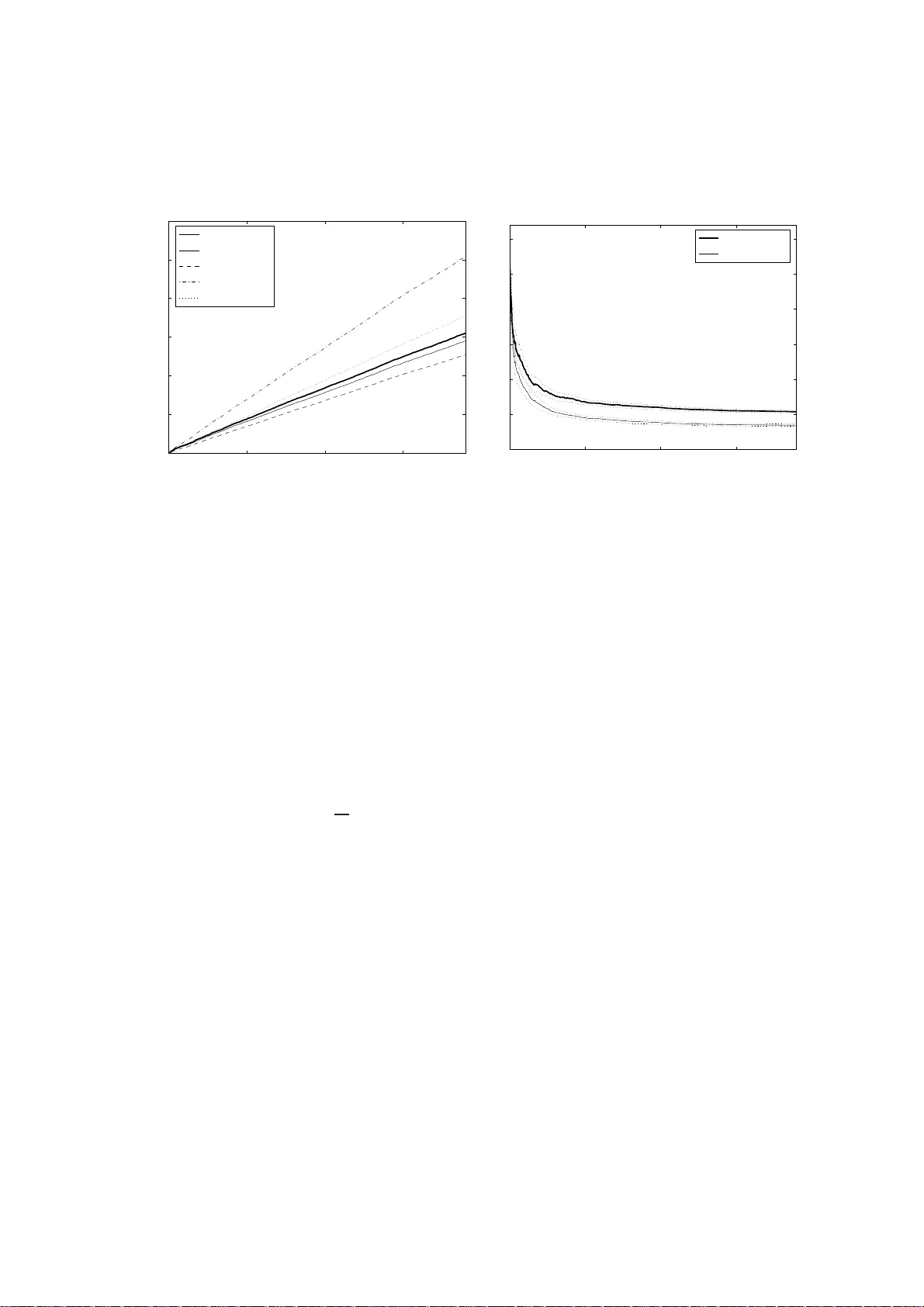
Algorithm Selection as a Bandit Pr oblem with Unbou nded Losses Matteo Gagliolo J ¨ urgen Schmidhuber T echnical Report No. IDSIA-07-08 July 9, 2008 IDSIA / USI-SUPSI Istituto Dalle Molle di studi sull’intelli genza a rtificiale Galleria 2, 6928 Manno, Switzerland IDSIA was founded by the Fondaz ione Dalle Molle per la Qualit ` a della V ita and is affilia ted with both the Univ ersit ` a della Svizzera italiana (USI) and the Scuola un versi taria professiona le della Svizzera italia na (SUPSI). Both authors are also af filiated with the Univ ersity of L ugano, Faculty of Informatics (V ia Buffi 13, 6904 Lugano, Switzerland). J. Schmidhuber is also af filiated with TU Munich (Boltzmannstr . 3, 85748 Garching , M ¨ unchen, Germany ). This work wa s supported by the Hasler foundation with grant n. 2244 . T echnical Report No. IDSIA-07-0 8 1 Algorithm Selectio n as a Bandit Problem with Unbou nded Losses Matteo Gagliolo J ¨ urgen Schmidhub er July 9, 2008 Abstract Algorithm selection is typically based on models of algo rithm p erformance, learned during a separate offline training sequence, which can be prohibiti vely expensi ve. In recent work, we adopted an online approach, in which a performance mod el is iterati vely updated and used to guide selection on a sequ ence of problem instances. The resulting explor ation-exploitation trade-of f was r epresented as a bandit prob- lem with exp ert advice, using an e xisting solv er for this game, but this required the setting of an arbitrary bound on algorithm runtimes, thus in validating the optimal re gret of the solver . In this pa per , we propo se a simpler framew ork for representing algorithm selection as a bandit problem, wit h partial information, and an unknown bound on losses. W e adapt an existing solver t o t his game, proving a bound on i ts ex- pected r egret, which holds also f or t he resulting algorithm selection technique. W e present preliminary experimen ts with a set of SA T solv ers on a mixed SA T -UNSA T benchma rk. 1 Introd uction Decades of research in the fields o f Ma chine Lea rning and Artificial I ntelligence bro ught us a variety of alternative algorithms for solving many k inds of p roblem s. Algorithms often display variability in perfor mance q uality , and comp utational c ost, d epend ing on th e particular prob lem in stance being solved: in o ther words, there is no single “best” algorithm. While a “trial an d er ror” appr oach is still the most popular, attem pts to automate alg orithm selection are n ot new [33], and ha ve grown to fo rm a consistent and dynamic field of research in th e area of Meta-Learning [ 37]. Many selection metho ds follow a n offline learning schem e, in which the availability of a large training set of per forman ce data for th e different algorithm s is assumed. Th is data is used to learn a model that maps ( pr o blem , algorithm ) pairs to expected perfor mance, or to some prob ability distribution on perf orman ce. The mod el is later used to select and run, for each new problem instance, only the algo rithm that is expe cted to giv e the best results. While this approa ch might so und reaso nable, it actually ignores the computation al co st of the initial training phase: collecting a representative sample of performan ce data has to be done via solving a set of training problem instances, and each instance i s solved rep eatedly , at least once for each of the av ailable algorithms, o r more if the algo rithms are randomized. Furthermo re, these training instances are assumed to be representative of future ones, as the model is not updated after training . In othe r words, there is an obvious trade-off between the e xploration of algorithm per forman ces o n different problem instances, aimed at learning the mo del, and the exploitation of the best algorithm/p roblem combinatio ns, b ased on the mo del’ s pr edictions. This trade-off is typically ign ored in of fline algo rithm selection, and the size of the training set is chosen heuristically . In our pre vious w ork [13, 14, 15], we have kept an online view of algor ithm selection, in which the o nly input av ailable to the m eta-learner is a set of algorithm s, of un known performance, and a sequenc e of pr oblem instances that h ave to be solved. Rather than artificially subd ividing the pro blem set into a training a nd a test set, we iteratively update the m odel each time an instance is solved, and use it to guide algorithm selection on the next instance. T echnical Report No. IDSIA-07-0 8 2 Bandit problems [3] offer a solid theoretical framework f or dealing with the exploratio n-exploitation trade-off in an o nline setting. One imp ortant obstacle to the straig htforward a pplication of a b andit p rob- lem solver to alg orithm selection is th at most existing solvers assume a bound on losses to be a vailable beforeh and. In [16, 15] w e d ealt with this issue heuristically , fixing th e b ound in advance. In this paper, we introd uce a mo dification of an existing b andit pro blem so lver [ 7], wh ich allows it to deal with an u n- known boun d on losses, while retaining a bound on the expected regret. This allo ws us to propose a simpler version of the algorithm selectio n framew ork G A M B L E T A , originally in trodu ced in [15]. The r esult is a parameterle ss online algorithm selection method, the first, to our knowledge, with a provable u pper bound on regret. The rest o f the p aper is o rganized as follows. Section 2 describes a ten tativ e taxo nomy of alg orithm selection methods, along with a fe w examples from literature. Section 3 pre sents our framew ork for repre- senting algor ithm selectio n as a b andit prob lem, d iscussing the in troductio n of a higher level of selection among different alg orithm selection techniques ( time allocators ). Section 4 introduces the modified bandit problem solver f or unbounded loss games, a long with its bound on regret. Section 5 describes experiments with SA T solvers. Section 6 concludes the paper . 2 Related work In gen eral terms, algorithm selection ca n be defined as the p rocess of allocating compu tational resources to a set of alter native algo rithms, in o rder to improve some measure of perfo rmance on a set of p roblem instances. Note that this definition includ es parameter selection: the alg orithm set can contain multip le copies o f a same alg orithm, d iffering in th eir p arameter setting s; or ev en iden tical r andomiz ed algorithms differing only in their random seeds. Algorith m selection techniques can be further described according to different orthogonal features: Decision vs. optimisatio n problems. A first distinctio n n eeds to be made among decision pro blems, where a binary criterion for recognizing a solution is a vailable; and op timisation problems, wh ere dif ferent lev els of solution q uality can b e attain ed, measu red by an objective f unction [2 2]. Literature on alg orithm selection is often focused on one of these two classes of pro blems. The selection is no rmally aimed at min- imizing solution tim e for d ecision prob lems; and at maximizing perf ormance quality , or improving som e speed-qu ality trade-off, for optimisation problems. Per set vs. per instance selection. The selection among different algorithm s ca n be performed once for an entire set of problem instances ( p er set selection, following [24]); or r epeated for each instance ( per instance selection). Static vs. dy namic selection. A further indep endent distinction [31] can b e made amon g static algorithm selection, in which a llocation of resources pr ecedes algorith m execution; and dynamic , or r eactive , algo- rithm selection, in which the allocation can be adapted during algorithm execution. Oblivious vs. non-o blivious selection. In oblivious techniq ues, algorithm selection is perform ed from scratch for each problem instance; in non-oblivio us technique s, there is some knowledge transfer acro ss subsequen t problem instances, usually in the form of a model of algorithm perform ance. Off-line vs. online learning. No n-ob li viou s techniq ues can be fu rther distinguish ed as offline or b atch learning techniques, where a separate trainin g pha se is performed , af ter wh ich the selection criteria are kept fixed; and online techniques, where the criteria can be updated e very time an instance is solved. A seminal p aper in the field o f algorithm selection is [3 3], in which offline, per instan ce selection is first pro posed, for both decisio n and o ptimisation p roblem s. Mo re recently , similar concepts have been propo sed, with d ifferent terminology (algor ithm r ecommenda tion , ranking , model selection ), in the Meta- Learning co mmun ity [ 12, 3 7, 18]. Research in this field usually deals with optimisation prob lems, an d is focu sed on maxim izing solution qua lity , witho ut taking into account the com putation al aspect. W ork on Empirica l Hardness Models [27, 30] is instead applied to decision prob lems, and f ocuses on obtaining accurate m odels o f runtime perf orman ce, condition ed o n numerous featu res of the problem instances, as T echnical Report No. IDSIA-07-0 8 3 well as on parame ters o f the solvers [24]. The models are used to perf orm a lgorithm selection on a per instance basis, and a re lear ned o ffline: online selection is a dvocated in [2 4]. Literature on algorithm port- folios [ 23, 19, 32] is usua lly fo cused on ch oice criteria f or building the set o f ca ndidate solvers, such that their areas of good p erform ance d o no t overlap, an d optimal static allocation of compu tational resour ces among elements of the portfo lio. A number of interesting d ynamic exceptions to the static selection paradig m have been prop osed re - cently . In [25], algo rithm perform ance modeling is based on the behavior of the candid ate algorithms dur- ing a p redefined amount of time, c alled the o bservationa l horizon , and dynamic co ntext-sensitiv e restart policies for SA T solvers ar e pr esented. In both cases, th e model is learned offline. I n a Reinforcemen t Learning [36] setting , algor ithm selection can be formulated as a Markov Dec ision Process: in [2 6], the algorithm set inc ludes sequences of recursiv e algorithms, fo rmed dynamica lly at run-time solving a seq uen- tial de cision prob lem, and a variation of Q- learning is used to find a dynam ic algo rithm selection policy; the resulting techniqu e is p er instance, dy namic and online. In [31], a set o f deterministic algorithm s is considered , and, und er some limitations, static and dynamic schedules are obtained , based o n dynamic progr amming. In both cases, the method presented is per set, offline. An ap proach b ased on runtime distributions can be fo und in [10, 11], for para llel indepen dent proc esses and shar ed reso urces resp ectiv ely . The run time distributions are assumed to be known, a nd the expected value o f a cost fu nction, acco unting for both wall-clock time an d resources usage, is minimized. A dy- namic schedu le is e valuated offline, using a bran ch-and -boun d algorithm to find th e optim al on e in a tr ee of possible schedules. Example s of allocation to two pro cesses are presen ted with artificially gen erated runtimes, and a real Latin squ are solver . Unfor tunately , the computation al comp lexity o f the tree sear ch grows e xpon entially in the number of processes. “Low-knowledge” oblivious ap proach es can be foun d in [4, 5], in whic h various simple ind icators of current solution improvement are used for algorithm selection, in order to achieve the best solution quality within a giv en tim e co ntract. In [ 5], the selection process is dynam ic: mac hine time shares are based o n a rece ncy-weighted a verage of p erform ance improvements. W e ado pted a similar approach in [13], where we consider ed algorithms with a scalar state, that had to reach a target v alue. The tim e to solution was estimated based on a shifting-wind ow linear extrapolation of the learning curves. For o ptimisation problems, if selection is only aimed at maximizing solution quality , the same problem instance can be so lved multiple times, keeping only the best solu tion. In this case, alg orithm selection can be r epresented as a Max K -armed band it prob lem, a variant of th e g ame in wh ich the rew ard attr ibuted to each arm is the m aximum payoff on a set of rounds. Solvers fo r this game are used in [9, 35] to imp lement oblivious per instance selection from a set of multi-start op timisation techn iques: each problem is treated indepen dently , and multiple runs o f the a vailable solvers are allocated, to m aximize perf orman ce quality . Further references can be found in [15]. 3 Algorithm selection as a bandit prob lem In its most b asic fo rm [34], the multi-armed band it problem is faced by a g ambler, playing a sequence of trials against an N -armed slot machin e. At each trial, the g ambler cho oses one of th e available arms, whose losses are random ly generated fr om different stationary distributions. The gam bler incurs in the correspo nding loss, and, in th e full information gam e, sh e can ob serve the losses that would ha ve b een paid pulling any of the other arms. A more optimistic formulation c an be made in terms of positiv e rewards. The aim of t he game is to m inimize the r e gr et , defined as t he difference between t he cumu lativ e lo ss of the gambler, an d the one of th e best arm. A b andit problem solver (B PS ) can be d escribed as a map ping from the history of th e observed losses l j for each arm j , to a probability distrib ution p = ( p 1 , ..., p N ) , fro m which the choice for the successi ve trial will be picked. More rece ntly , th e original r estricting assump tions h ave been pro gressively relaxed, allowing for non- stationary loss distributions, partial inform ation (only the loss for the pulled arm is observed), and a dver- T echnical Report No. IDSIA-07-0 8 4 sarial bandits that can set their losses in order to decei ve the player . In [2, 3], a re ward game is considered, and no statistical assum ptions are made abou t the process gener ating the rew ards, which are a llowed to be an arbitrary fun ction of the entire history o f the game ( non- obliviou s adversarial settin g). Based on these pessimistic hypo theses, the author s describe probab ilistic gam bling strategies fo r the full an d the partial informa tion games. Let us now see how to represent algor ithm selection f or d ecision pr oblems as a bandit p roblem, with the aim of minimizing solution time. Consider a sequence B = { b 1 , . . . , b M } of M instances of a decision problem , for w hich we want to min imize solution time, and a set of K alg orithms A = { a 1 , . . . , a K } , such that each b m can be solved by each a k . It is straig htforward to d escribe static algorithm selection in a multi-armed ba ndit setting , where “pick arm k ” means “r un algorithm a k on n ext problem instance”. Runtimes t k can be viewed as losses, generated b y a rather complex m echanism, i. e., the algorith ms a k themselves, running on the current problem. The information is partial, as the runtime for other algorithms is not av ailable, unless we d ecide to so lve th e same problem instance again. In a worst case scena rio o ne can receive a ” deceptive” problem sequence, starting with problem instances on which the perform ance of the algo rithms is misleading, so this b andit pro blem should b e consid ered adversarial. As B P S typically minimize the regret with respect to a sing le arm, this ap proach w ould allo w to implement per set selectio n, of the overall best algorith m. An example can b e fou nd in [ 16], w here we p resented an online m ethod for learning a per set estimate of an optimal restart strategy . Unfortu nately , p er set selection is o nly pro fitable if o ne of the algorithms do minates the others on all problem instances. This is usually not the case: it is often o bserved in practice that different algorithm s perfor m b etter on different prob lem instances. In this situation, a per instance s election scheme, which can take a different d ecision for each problem instance, can have a great advantage. One possible way of e xploitin g the nice theoretical pr operties of a B P S in the co ntext of alg orithm selection, w hile allowing for th e imp rovement in perfo rmance of per instance selectio n, is to u se the B P S at an upper le vel, to select among alternative algorith m selection techniques. Consider again the algorithm selection problem repre sented by B an d A . Introd uce a set of N time alloca tors (T A j ) [13, 15]. Each T A j can be an arb itrary fun ction, mapping the c urrent history of collected perfor mance data for e ach a k , to a share s ( j ) ∈ [0 , 1] K , with P K k =1 s k = 1 . A T A is used to solve a giv en problem instance executing all algorithm s in A in parallel, on a single machine , whose compu tational resourc es ar e allocated to each a k propo rtionally to the corresp onding s k , such tha t for any p ortion of time sp ent t , s k t is u sed by a k , as in a static algor ithm por tfolio [2 3]. The runtim e be fore a solution is fou nd is th en min k { t k /s k } , t k being the runtime of algorithm a k . A trivial examp le o f a T A is the uniform time allocator , assigning a con stant s = (1 / K , ..., 1 / K ) . Single algorithm selectio n can be represen ted in this framework by settin g a single s k to 1 . Dy namic allocato rs will pro duce a time-varying sh are s ( t ) . In previous work, we presented examp les of heuristic oblivious [13] and no n-oblivious [14] allocators; mo re soun d T As are prop osed in [15], b ased on n on-p arametric models of the runtime distrib ution of the algorithms, which are used to minimize th e exp ected v alue of so lution time, or a quan tile of this quantity , or to maximize solution probability within a giv e time contract . At this higher level, one can use a B P S to select amon g different time allocators, T A j , T A 2 . . . , working on a same algorithm set A . I n this ca se, “p ick arm j ” mea ns “use time allocator T A j on A to solve next problem instance”. In the long term, the B P S would allow to select, on a per set basis, the T A j that is best at allocating time to algorith ms in A on a per instance basis. The resulting “Gambling ” Time Allocator ( G A M B L E TA) is described in Alg. 1. If B P S allows fo r non-stationary ar ms, it can also deal with time allocators that are learning to allocate time. This is actually the o riginal moti vation for adopting th is two-level selection scheme, as it allows to co mbine in a prin cipled way the exploration of algo rithm b ehavior , wh ich can be repr esented by the unifor m time allocator , an d th e exploitation of this inf ormation b y a model-based allocato r , whose m odel is being lear ned online, based on results o n the sequence of prob lems met so far . If mor e time a llocators are av a ilable, they can be made to com pete, using the B P S to explore their performa nces. Ano ther interesting feature o f this selection scheme is that the initial r equirem ent that each algor ithm shou ld be capable of T echnical Report No. IDSIA-07-0 8 5 Algorithm 1 G A M B L E T A ( A , T , B P S ) Gambling Time Allocator . Algorithm set A with K algorithms; A set T o f N time allocators T A j ; A bandit problem solver B P S M problem instances. initialize B P S ( N , M ) for each problem b i , i = 1 , . . . , M do pick time allocator I ( i ) = j with probab ility p j ( i ) from B P S. solve problem b i using T A I on A incur loss l I ( i ) = min k { t k ( i ) /s ( I ) k ( i ) } update B P S end for solving each problem can be relaxed, requiring instead that at least one of th e a k can solve a gi ven b m , and that e ach T A j can solve each b m : this can be ensured in practice by imp osing a s k > 0 for all a k . This allows to use interesting combinations of complete an d incomplete solvers in A (see Sect. 5). Note that any bound o n the regret of the B P S will determ ine a bound on the regret of G A M B L E T A with respect to the best time allo cator . Nothing can be said about the performan ce w .r .t. the b est algorith m. In a worst-c ase setting, if no ne of the time allocator is effecti ve, a bound can still be obtained by includin g the u niform share in th e set o f T As. In practice, though, per -instance selection can be mu ch more ef ficient t han unifor m allocation, and the literature is full of examples of time allocators which e ventually conv erge to a good perfor mance. The orig inal version o f G A M B L E T A ( G A M B L E T A 4 in the f ollowing) [15] was based o n a more c om- plex a lternative, inspired by the b andit problem with expert ad vice, as descr ibed in [2, 3 ]. I n that setting, two games are g oing on in parallel: at a lower le vel, a partial info rmation game is p layed, b ased on the probab ility distribution obtained mixing the advice of different experts , repr esented as p robab ility d istri- butions on the K arms. Th e exper ts can be arbitr ary fu nctions of the histor y of observed rewards, and giv e a d ifferent advice for each trial. At a higher le vel, a full information game is play ed, with the N experts p laying the roles of th e different arm s. Th e probability d istribution p at this level is not used to pick a sing le exper t, b ut to mix their ad vices, in order to g enerate the d istribution for the lower lev el arms. In G A M B L E T A 4 , the time allocato rs p lay the role of the experts, each sugg esting a different s , on a per instance basis; and th e a rms of the lower level gam e are the K algorithm s, to be run in parallel with the mixture share. E X P 4 [ 2, 3] is u sed a s the BP S . Unf ortunately , th e b ound s for E X P 4 cannot be extended to G A M B L E T A 4 in a straightforward manner , as the lo ss fun ction itself is not co n vex; mor eover , E X P 4 cannot deal with unbou nded losses, so we h ad to ado pt an he uristic rew ard attribution instead of u sing the plain runtimes. A common issue of the above ap proach es is the difficulty o f setting reasonable upper bounds on the time required by the algorithm s. This rende rs a straightforward application of most B P S pr oblematic, as a known bo und on losses is u sually ass umed , an d used to tune par ameters of the so lver . Und erestimating this bound can in validate the bo unds o n regret, w hile overestimating it can p roduce an excessi vely ”cau tious” algorithm , with a po or performance. Setting in adv ance a good bound is particu larly dif ficult when dealing with alg orithm runtimes, which can easily exhibit variations of sev eral or der of m agnitud es among different problem instances, or e ven among different runs on a same instance [20]. Some interesting r esults regarding games with unboun ded lo sses hav e recently b een obtained. In [7, 8] , the au thors co nsider a full in formatio n game, and provid e two algo rithms which can adapt to unk nown bound s on signed rewards. Based on th is w ork, [1] provide a Hannan con sistent algorithm fo r losses wh ose bound g rows in th e number of trials i with a known r ate i ν , ν < 1 / 2 . This latter hy pothesis do es n ot fit well T echnical Report No. IDSIA-07-0 8 6 our situation , a s we would like to av oid a ny restrictio n on the seq uence o f p roblems: a very h ard instan ce can be m et first, followed by an easy one. In this sense, the hypothesis of a c onstant, but unk nown, bound is more suited. In [7], Cesa-Bian chi et al. also introduce an algorithm for loss games with partial informatio n ( E X P 3 L I G H T ), which requires losses to be bound, and is particularly ef fectiv e when th e cumulati ve loss of the best a rm is small. In the n ext section we introdu ce a variation of this algor ithm that allo ws it to deal with an unknown bound on losses. 4 An algorithm f or games with an unknow n bound on losses Here and in t he following, we consid er a partial information game with N arm s, and M trials; an index ( i ) indicates the value o f a quantity used or observed a t tr ial i ∈ { 1 , . . . , M } ; j indicate quan tities r elated to the j -th arm, j ∈ { 1 , . . . , N } ; index E refe rs to the lo ss incu rred by the bandit pr oblem solver , and I ( i ) indicates the ar m chosen at trial ( i ) , so it is a discr ete rando m v ariable with value in { 1 , . . . , N } ; r , u will represent quantities related to an epoch o f the ga me, which co nsists of a sequence o f 0 o r more co nsecutive trials; log with no index is the natural logarithm . E X P 3 L I G H T [7, Sec. 4] is a solver fo r the band it lo ss game with p artial inform ation. It is a m odified version of the weighted ma jority algorith m [29], in whic h the cumula ti ve losses for each arm are obtaine d throug h an un biased estimate 1 . The game con sists of a sequ ence of epochs r = 0 , 1 , . . . : in ea ch epo ch, the pro bability d istribution over the arms is upd ated, pro portio nal to exp ( − η r ˜ L j ) , ˜ L j being the curren t unbiased estimate of the cumula ti ve loss. Assumin g an upper bound 4 r on the smallest loss estimate, η r is set as: η r = s 2(log N + N lo g M ) ( N 4 r ) (1) When this boun d is first trespassed, a ne w epoch starts and r and η r are updated accordin gly . The original algorithm assumes losses in [0 , 1 ] . W e first co nsider a game with a k nown finite bound L on losses, and in troduce a slightly mo dified version of E X P 3 L I G H T (Alg orithm 2), obtained simply dividing all losses by L . Based on Theorem 5 from [7], it is easy to prove the fo llowing Theorem 1. If L ∗ ( M ) is the loss of the best arm after M tria ls, and L E ( M ) = P M i =1 l I ( i ) ( i ) is the loss of E X P 3 L I G H T ( N , M , L ) , the expected value of its r e gr et is bounded as: E { L E ( M ) } − L ∗ ( M ) (2) ≤ 2 p 6 L (log N + N lo g M ) N L ∗ ( M ) + L [2 p 2 L (log N + N lo g M ) N + (2 N + 1)(1 + log 4 (3 M + 1))] The proof is tri vial, and is given in the appendix. W e now introduce a simple variation of Algorith m 2 which does n ot require the kn owledge of the bound L on losses, and uses A lgorithm 2 as a subrou tine. E X P 3 L I G H T - A (Algorithm 3) is inspired by the dou bling trick used in [7] for a fu ll info rmation game with un known b ound on losses. The game is again organized in a sequence of epoch s u = 0 , 1 , . . . : in each epoch, Algorithm 2 is r estarted using a bound L u = 2 u ; a n ew epoch is started with the a pprop riate u whe never a loss larger than th e cur rent L u is observed. 1 For a giv en round, and a gi ven arm with lo ss l and pull probabili ty p , the estimat ed loss ˜ l is l/p if the arm is pull ed, 0 otherwise. This estimate is unbiased in the sense that its expect ed val ue, with respect to the process extra cting the arm to be pulled, equals the actua l va lue of the loss: E { ˜ l } = p l/p + (1 − p )0 = l . T echnical Report No. IDSIA-07-0 8 7 Algorithm 2 E X P 3 L I G H T ( N , M , L ) A solver for bandit pro blems with partial information and a k nown bound L on lo sses. N arms, M trials losses l j ( i ) ∈ [0 , L ] ∀ i = 1 , ..., M , j = 1 , . . . , N initialize epoch r = 0 , L E = 0 , ˜ L j (0) = 0 . initialize η r accordin g to (1) for each trial i = 1 , ..., M do set p j ( i ) ∝ exp( − η r ˜ L j ( i − 1) / L ) , P N j =1 p j ( i ) = 1 . pick arm I ( i ) = j with prob ability p j ( i ) . incur loss l E ( i ) = l I ( i ) ( i ) . ev a luate unbiased loss estimates: ˜ l I ( i ) ( i ) = l I ( i ) ( i ) /p I ( i ) ( i ) , ˜ l j = 0 f or j 6 = I ( i ) update cumulative losses: L E ( i ) = L E ( i − 1) + l E ( i ) , ˜ L j ( i ) = ˜ L j ( i − 1) + ˜ l j ( i ) , for j = 1 , . . . , N ˜ L ∗ ( i ) = min j ˜ L j ( i ) . if ( ˜ L ∗ ( i ) / L ) > 4 r then start next epoch r = ⌈ log 4 ( ˜ L ∗ ( i ) / L ) ⌉ update η r accordin g to (1) end if end for Algorithm 3 E X P 3 L I G H T - A ( N , M ) A solver fo r bandit problem s with partial information and an unknown (but finite) bound on losses. N arms, M trials, losses l j ( i ) ∈ [0 , L ] ∀ i = 1 , ..., M , j = 1 , . . . , N unknown L < ∞ initialize epoch u = 0 , E X P 3 L I G H T ( N , M , 2 u ) for each trial i = 1 , ..., M do pick arm I ( i ) = j with prob ability p j ( i ) from E X P 3 L I G H T . incur loss l E ( i ) = l I ( i ) ( i ) . if l I ( i ) ( i ) > 2 u then start next epoch u = ⌈ log 2 l I ( i ) ( i ) ⌉ restart E X P 3 L I G H T ( N , M − i, 2 u ) end if end for T echnical Report No. IDSIA-07-0 8 8 Theorem 2. If L ∗ ( M ) is the lo ss of th e best arm after M trials, a nd L < ∞ is the u nknown bound on losses, the expected value of the r e gr et of E X P 3 L I G H T - A ( N , M ) is bo unded as: E { L E ( M ) } − L ∗ ( M ) ≤ (3) 4 p 3 ⌈ log 2 L⌉L (log N + N log M ) N L ∗ ( M ) + 2 ⌈ lo g 2 L⌉L [ p 4 L (log N + N lo g M ) N + (2 N + 1)(1 + log 4 (3 M + 1)) + 2] The proof is gi ven in th e appendix . Th e regret obtained by E X P 3 L I G H T - A is O ( p L N log M L ∗ ( M )) , which can b e usefu l in a situation in wh ich L is high but L ∗ is relatively sma ll, as we expect in ou r time allocation setting if the alg orithms exhibit huge variations in ru ntime, b ut at least one of the T As e ventually conv erges to a goo d performance. W e can then use E X P 3 L I G H T - A as a B P S fo r selecting among dif feren t time allocators in G A M B L E T A ( Algorithm 1). 5 Experiments The s et of time a llocator used in the following experime nts is the same as in [15], and includes t he uniform allocator, along with nin e o ther dynamic allocators, optimizing dif feren t quantiles of run time, based on a nonparam etric model of the runtime distrib ution that is u pdated after each p roblem is solved. W e first briefly describe these time allocato rs, inviting the reader to refer to [15] for fu rther details and a d eeper discussion. A sep arate mod el F k ( t | x ) , cond itioned on features x of the pro blem instance, is used for each algorithm a k . Based on th ese mo dels, the runtime distribution fo r the whole algo rithm portf olio A can be ev a luated for an arbitrary share s ∈ [0 , 1] K , with P K k =1 s k = 1 , as F A , s ( t ) = 1 − K Y k =1 [1 − F k ( s k t )] . (4) Eq. (4) can be used to evaluate a qu antile t A , s ( α ) = F − 1 A , s ( α ) fo r a gi ven solution probability α . Fixing this value, t ime is allocated using the share that minimize s the quantile s = arg min s F − 1 A , s ( α ) . (5) Compared to m inimizing expected runtime , this time allocator has th e advantage of being ap plicable even when the runtime distributions are improper, i. e. F ( ∞ ) < 1 , as in the case of inco mplete solvers. A dynamic version of th is time allocator is obtain ed updating the share value perio dically , condition ing each F k on the time spent so far by the correspond ing a k . Rather than fi xing an arbitrary α , we used nine dif feren t instan ces of this time allocator, with α ra nging from 0 . 1 to 0 . 9 , in addition to the unifor m allocator, an d let the B P S select the best one. W e present experimen ts for the algorith m selection scen ario fr om [15], in which a local search and a complete SA T solver (respecti vely , G2-WSA T [2 8] and Satz-Rand [20]) are com bined to solve a sequence of ran dom satisfiable an d unsatisfiable p roblem s ( benchm arks uf- * , uu - * from [21], 1899 instances in total). As th e clauses-to-variable ratio is fixed in this benchmark, only the num ber o f variables, r anging from 20 to 250 , was used as a problem feature x . Local search algorithm s are mo re efficient on satisfi- able instances, b ut cannot prove un satisfiability , so are d oomed to ru n for ev er o n unsatisfiable instan ces; while comp lete solvers are guara nteed to termin ate their execution on all instances, as they can also p rove unsatisfiability . For the whole pro blem sequenc e, the overhead o f G A M B L E T A 3 (Alg orithm 1, using E X P 3 L I G H T - A as the B P S ) over an idea l “oracle”, which can predict and r un o nly the fastest algorithm, is 22% . G A M - B L E T A 4 (fro m [15], b ased on E X P 4 ) seems to pro fit from th e mix ing of time alloc ation shares, o btaining T echnical Report No. IDSIA-07-0 8 9 0 500 1000 1500 0 1 2 3 4 5 6 x 10 10 Task sequence Cumulative time [cycles] (a) cumulative time GambleTA3 GambleTA4 Oracle Uniform Single 0 500 1000 1500 0 0.2 0.4 0.6 0.8 1 1.2 Task sequence Cumulative overhead (b) cumulative overhead GambleTA3 GambleTA4 Figure 1: (a): Cumulati ve time spent by G A M B L E TA 3 and G A M B L E T A 4 [15] on the SA T -UNSA T problem set ( 10 9 ≈ 1 min.). Upp er 95% confidence bounds on 20 runs, with random reordering of t he problems. O R A C L E is the lo wer bound on performance. U N I F O R M is the ( 0 . 5 , 0 . 5 ) share. S A T Z - R A N D is the per-set best algorithm. (b): The e volution of cumulati ve ove rhead, defined as ( P j t G ( j ) − P j t O ( j )) / P j t O ( j ) , where t G is the performance of G A M B L E TA and t O is the performance of the oracle. Dotted lines represent 95% confidence bounds. a better 14% . Satz-Ran d alone can solve all the problems, b ut with an overhead of about 4 0% w .r .t. the oracle, due to its po or pe rforma nce on satisfiable instan ces. Fig. 1 plots the evolution of cumulative time, and cumulative overhead , a long the prob lem s equen ce. 6 Conclusions W e presented a ban dit problem solver for loss games with partial inf ormation and an unknown bou nd on losses. T he solver represen ts an ideal plu g-in for our algorithm selectio n meth od G A M B L E TA, a voiding the n eed to set a ny addition al parameter . The choice of the alg orithm set and time allocator s to use is still left to the user . Any existing s election techn ique, including obli vious ones, can be included in the set of N allocators, with an impact O ( √ N ) on the regret: th e overall performan ce of G A M B L E T A will conver ge to the o ne of the best time allocator . Preliminary experiments showed a degradation in performa nce compar ed to the heuristic version presented in [15], which requires to set in advance a maximum runtime, and cannot be provided of a bound on re gret. According to [6], a bo und for the original E X P 3 L I G H T can be proved for an adaptive η r (1), in which the total number of trials M is replaced by the current trial i . This shou ld allow for a potentially mo re efficient variation of E X P 3 L I G H T - A , in wh ich E X P 3 L I G H T is not restarted at each epoch , and can retain the informatio n on past losses. One potential advantage of of fline selection methods is that the initial training phase can be easily par- allelized, distributing the workload on a cluster of m achines. Ongoin g r esearch aims at extendin g G A M - B L E T A to allocate multip le CPUs in par allel, in ord er to obtain a fu lly distributed algorithm selection framework [17]. Acknowledgments. W e would like to thank Nicol ` o Cesa-Bianchi for contributing the proofs fo r E X P 3 L I G H T and useful rema rks o n h is w ork, and F austino Gomez f or his comm ents on a dr aft o f th is paper . This work w as suppo rted by the Hasler foundation with grant n. 2244 . T echnical Report No. IDSIA-07-0 8 10 Refer ences [1] Chamy Allenb erg, Peter Auer , L ´ aszl ´ o Gy ¨ orfi, an d Gy ¨ orgy Ottucs ´ ak. Hann an consistency in on-line learning in case of unbo unded losses under p artial m onitorin g. In Jos ´ e L. Balc ´ azar et al., editors, ALT , volume 4264 of Lectur e Notes in Computer Science , pages 229– 243. Springer , 2006. [2] Peter Auer , Nicol ` o Cesa-Bianchi, Y oav Fre und, and Robert E. Schapire. Ga mbling in a rigged casino: the adversarial multi-armed bandit problem. I n Pr ocee dings of the 36th Annual Symposium on F oun- dations of Comp uter Scien ce , pages 322 –331 . IE EE Computer Society Press, Los Alam itos, CA, 1995. [3] Peter Auer, Nicol ` o Cesa-Bianchi, Y oav Freund , and Rob ert E. Schapire . The nonstocha stic mu lti- armed bandit problem. SIAM J . Comput. , 32(1) :48–77 , 200 3. [4] Christoph er J. Beck and Eugene C. Freu der . Simple ru les for low-knowledge algo rithm selection. In CP AIOR , pages 50–6 4, 2004. [5] T . Carchrae and J. C. Beck. Ap plying machine learning to low knowledge control of optimization algorithm s. Compu tational Intelligence , 21(4):3 73–38 7, 2005 . [6] Nicol ` o Cesa-Bianchi. Personal communicatio n, 2008. [7] Nicol ` o Cesa-Bianchi, Y ishay M ansour, and Gilles Stoltz. Improved second-orde r bounds for pr edic- tion with expert advice . In Peter Auer, Ron Meir, Peter Auer, and Ron Meir , ed itors, COLT , volume 3559 of Lectur e Notes in Computer Science , pages 217–2 32. Springer, 20 05. [8] Nicol ` o Cesa-Bianchi, Y ishay M ansour, and Gilles Stoltz. Improved second-orde r bounds for pr edic- tion with expert advice. Machine Learning , 66(2- 3):321 –352 , March 2007. [9] V incen t A. Cicirello and Stephen F . Smith. Th e m ax k-armed b andit: A new mo del of explo ration applied to search heu ristic selection. I n T wentieth Natio nal Confer ence on Artificial Intelligence , pages 1355 –1361 . AAAI Press, 200 5. [10] Lev Finkelstein, Shaul Markovitch, and Ehud Rivlin. Optimal schedules for p arallelizing anytime algorithm s: the case of independ ent processes. In Eighteen th nationa l confer ence on Artificial in tel- ligence , pages 719–724 , Me nlo Park, CA, USA, 2002. AAAI Press. [11] Lev Finkelstein, Shaul Markovitch, and Ehud Rivlin. Optimal schedules for p arallelizing anytime algorithm s: The case o f sh ared resources. Journal of Artificial I ntelligence Researc h , 19:7 3–138 , 2003. [12] Johan nes F ¨ urnk ranz. On -line b ibliogra phy on m eta-learnin g, 2001. EU ESPRIT ME T AL Project (26.35 7): A Meta-Learn ing Ass istant for Providing User Support in Machine Learning Mining. [13] M. Gagliolo, V . Zhumatiy , and J. Schmidhuber . Adaptive on line time allo cation to search algorithms. In J.F . Boulicau t et al., editor, Machine Learning: ECML 200 4. Pr oceed ings of the 15th Eur opea n Confer ence o n Ma chine Learning, Pisa, Italy , Sep tember 20 -24, 2004 , pages 13 4–14 3. Springe r , 2004. [14] Matteo Gagliolo and J ¨ urgen S chmid huber . A neural network model f or inter -proble m adaptive onlin e time allo cation. In Włodzisław Du ch et al., ed itors, A rtificial Neural Networks: F ormal Mo dels a nd Their Applications - ICANN 2005 Pr oceed ings, P art 2 , pages 7–1 2. Springer , September 2005. [15] Matteo G agliolo an d J ¨ urgen Schm idhub er . Le arning dy namic algo rithm portf olios. Annals of Math- ematics and Artificial Intelligence , 47(3–4):2 95–3 28, August 2006 . AI&MA TH 2006 Special Issue. T echnical Report No. IDSIA-07-0 8 11 [16] Matteo Gaglio lo and J ¨ urgen Schmidhu ber . Learning restart strategies. In Manuela M. V eloso, editor, IJCAI 2007 — T wentieth Interna tional J oint Confer ence on Artificial In telligence, vol. 1 , pages 792– 797. AAAI Press, January 2007. [17] Matteo Gag liolo a nd J ¨ urgen Schmid huber . T owards distributed algorith m por tfolios. In DCAI 2008 — Interna tional S ymposium on Distributed Computing a nd A rtificial In telligence , Ad vances in Soft Computing . Springer, 20 08. T o appear . [18] Christop he Giraud-Carrier, Ricardo V ilalta, an d Pa vel Brazdil. Intr oductio n to the special issue on meta-learnin g. Machine Learning , 54(3) :187–1 93, 200 4. [19] Carla P . Gomes and Bar t Selman . Algorith m por tfolios. Artificial In telligence , 12 6(1–2 ):43– 62, 2 001. [20] Carla P . Gomes, Bart Selman, Nuno Crato, and Hen ry Kautz. Heavy-tailed pheno mena in satisfiability and constraint satisfaction problems. J. Autom. Reason. , 24(1-2):67 –100 , 2000. [21] H. H. Hoos an d T . St ¨ utzle. SA T LIB: An Online Resource for Research on SA T . In I.P . Gent et al., editors, SA T 2000 , pages 283–2 92, 2000. http://www.satli b.org . [22] Holg er H. Ho os and T homas St ¨ utzle. Local search algorithms for SA T: An empirical e valuation. Journal of A utoma ted Reasoning , 24(4):421 –481 , 2000. [23] B. A. Huberman, R. M. Lukose, and T . Hogg . An economic approach to hard compu tational p roblems. Science , 275:51 –54, 1997. [24] Frank Hutter and Y oussef Hamadi. Paramete r adjustment based on performan ce p rediction: T ow ards an in stance-aware problem solver . T ech nical Rep ort MSR-TR-20 05-1 25, Microsoft Research , Cam- bridge, UK, December 2005. [25] Henr y A. Kautz, Eric Horv itz, Y ongshao Ruan, Carla P . Gomes, a nd Bart Selman. Dynam ic restart policies. In AAAI/IAAI , pages 674–68 1, 2002. [26] Micha il G. Lagoudakis and M ichael L. Littman. A lgorithm selection using rein forceme nt learnin g. In Pr oc . 17th ICML , pages 511–51 8. Morgan Kaufmann, 2000. [27] Ke vin Leyton-Brown, Eugene Nu delman, an d Y o av Shoh am. Learning the empirical hardness of optimization p roblems: Th e case of co mbinator ial au ctions. In I CCP: In ternationa l Confe r ence on Constraint Pr ogramming (CP), LNCS , 2002. [28] Chu Min Li an d W enqi Huang. Diversification and dete rminism in local search fo r satisfiability . In SA T2005 , pages 158–172 . Springer, 20 05. [29] Nick Littlestone and Ma nfred K. W arm uth. The weig hted majo rity alg orithm. Inf. Comput. , 108(2 ):212– 261, 1994 . [30] Eug ene Nudelman , Ke v in Leyton -Brown, Holger H. Hoos, Alex Devkar , and Y oav Shoha m. Under- standing random sat: Beyond the clauses-to-variables ratio. In CP , p ages 438–4 52, 2004. [31] Marek Petrik. Statistically o ptimal combin ation o f algorithms. Presented at SOFSEM 2005 - 31st Annual Conference on Current T rends in Theory and Practice of Infor matics, 2005. [32] Marek Petrik and Shlomo Zilberstein. L earning static parallel portfolio s of alg orithms. N inth I nter- national Symposium on Artificial Intelligence and Mathematics., 2006. [33] J. R. Rice. The algorithm selection p roblem. In Morris Rubino ff and Ma rshall C. Y ovits, editor s, Advance s in computers , v olume 15, pages 65–11 8. Academic P ress, New Y ork, 1976 . T echnical Report No. IDSIA-07-0 8 12 [34] H. Robbins. Some aspects of the sequential design of e xper iments. Bulletin of the AMS , 58:527–53 5, 1952. [35] Matthew J. Streeter and Stephen F . Smith. An asymptotica lly optimal algorithm for the max k-armed bandit problem. In T wenty-F irst National Confer ence on Artificial Intelligence . AAAI Press, 2006. [36] R. Sutton and A. Barto. Reinfor cement le arning: An intr oduction . Camb ridge, MA, M IT Press, 1998. [37] Ricardo V ilalta and Y oussef Drissi. A perspectiv e vie w and surve y of meta-learn ing. Artif . Intell. Rev . , 18(2) :77–9 5, 20 02. A ppend ix A.1 Pr oof of Theore m 1 The pro of is trivially based on the r egret for the origin al E X P 3 L I G H T , with L = 1 , which ac cording to [7, Theorem 5] (proof obtained from [6]) can be ev aluated using the optimal v alues (1) for η r : E { L E ( M ) } − L ∗ ( M ) ≤ (6) 2 p 2(log N + N lo g M ) N (1 + 3 L ∗ ( M )) + (2 N + 1)(1 + log 4 (3 M + 1)) . As we are playing the same game normalizing all losses with L , the following will hold for Alg. 2: E { L E ( M ) } − L ∗ ( M ) L ≤ (7) 2 p 2(log N + N log M ) N (1 + 3 L ∗ ( M ) / L ) (8) + (2 N + 1)(1 + log 4 (3 M + 1)) . (9) Multiplying both sides for L an d rearranging produce s ( 2). A.2 Pr oof of Theore m 2 This follows the p roof technique emp loyed in [7, T heorem 4]. Be i u the last trial of ep och u , i. e. the first trial at which a loss l I ( i ) ( i ) > 2 u is ob served. Write cum ulative losses dur ing an ep och u , excluding the last t rial i u , as L ( u ) = P i u − 1 i = i u − 1 +1 l ( i ) , and let L ∗ ( u ) = min j P i u − 1 i = i u − 1 +1 l j ( i ) indicate the optimal lo ss for this subset o f trials. Be U = u ( M ) the a priori unknown epoch at the last trial. In each epoch u , the bo und (2) holds with L u = 2 u for all trials except the last o ne i u , so noting that log ( M − i ) ≤ log ( M ) we can write: E { L ( u ) E } − L ∗ ( u ) ≤ ( 10) 2 q 6 L u (log N + N log M ) N L ∗ ( u ) + L u [2 p 2 L u (log N + N log M ) N + (2 N + 1)(1 + log 4 (3 M + 1))] . The loss for trial i u can only be bound by the next v alue of L u , e valuated a posteriori : E { l E ( i u ) } − l ∗ ( i u ) ≤ L u +1 , (11) T echnical Report No. IDSIA-07-0 8 13 where l ∗ ( i ) = min j l j ( i ) indicates the optimal loss at trial i . Combining (10,11), and writing i − 1 = 0 , i U = M , we obtain the regret for the whole game: 2 E { L E ( M ) } − U X u =0 L ∗ ( u ) − U X u =0 l ∗ ( i u ) ≤ U X u =0 { 2 q 6 L u (log N + N log M ) N L ∗ ( u ) + L u [2 p 2 L u (log N + N log M ) N + (2 N + 1)(1 + log 4 (3 M + 1))] } + U X u =0 L u +1 . The first term on the right hand side of (12) can be bound ed using Jensen’ s inequ ality U X u =0 √ a u ≤ v u u t ( U + 1) U X u =0 a u , (12) with a u = 24 L u (log N + N log M ) N L ∗ ( u ) (13) ≤ 24 L U +1 (log N + N log M ) N L ∗ ( u ) . The othe r terms do not d epend on the o ptimal losses L ∗ ( u ) , and can also be bounded noting that L u ≤ L U +1 . W e n ow ha ve to b ound the num ber of epo chs U . This can be don e noting that the maximum ob served loss cannot be larger than the unknown, but finite, bound L , and that U + 1 = ⌈ lo g 2 max i l I ( i ) ( i ) ⌉ ≤ ⌈ log 2 L⌉ , (14) which implies L U +1 = 2 U +1 ≤ 2 L . (15) In this way we can bound the sum U X u =0 L u +1 ≤ ⌈ log 2 L⌉ X u =0 2 u ≤ 2 1+ ⌈ log 2 L⌉ ≤ 4 L . (16) W e conc lude by noting that L ∗ ( M ) = min j L j ( M ) (17) ≥ U X u =0 L ∗ ( u ) + U X u =0 l ∗ ( i u ) ≥ U X u =0 L ∗ ( u ) . 2 Note that a ll cumulati ve losses are counte d from trial i u − 1 + 1 to trial i u − 1 . If an epoc h ends on i ts first trial, (10) is zero, and (11) holds. Writing i U = M implies the wor st case hypothesi s that the bound L U is e xceeded on the la st trial. Epoch numbers u are increa sing, but not nece ssarily consecuti ve: in this case the terms relat ed to the missing epochs are 0 . T echnical Report No. IDSIA-07-0 8 14 Inequa lity (12) then becomes: E { L E ( M ) } − L ∗ ( M ) ≤ 2 p 6( U + 1) L U +1 (log N + N log M ) N L ∗ ( M ) + ( U + 1) L U +1 [2 p 2 L U +1 (log N + N log M ) N + (2 N + 1)(1 + log 4 (3 M + 1))] + 4 L . Plugging in (14, 15) and rearrang ing we obtain (3).