Improved Cheegers Inequality: Analysis of Spectral Partitioning Algorithms through Higher Order Spectral Gap

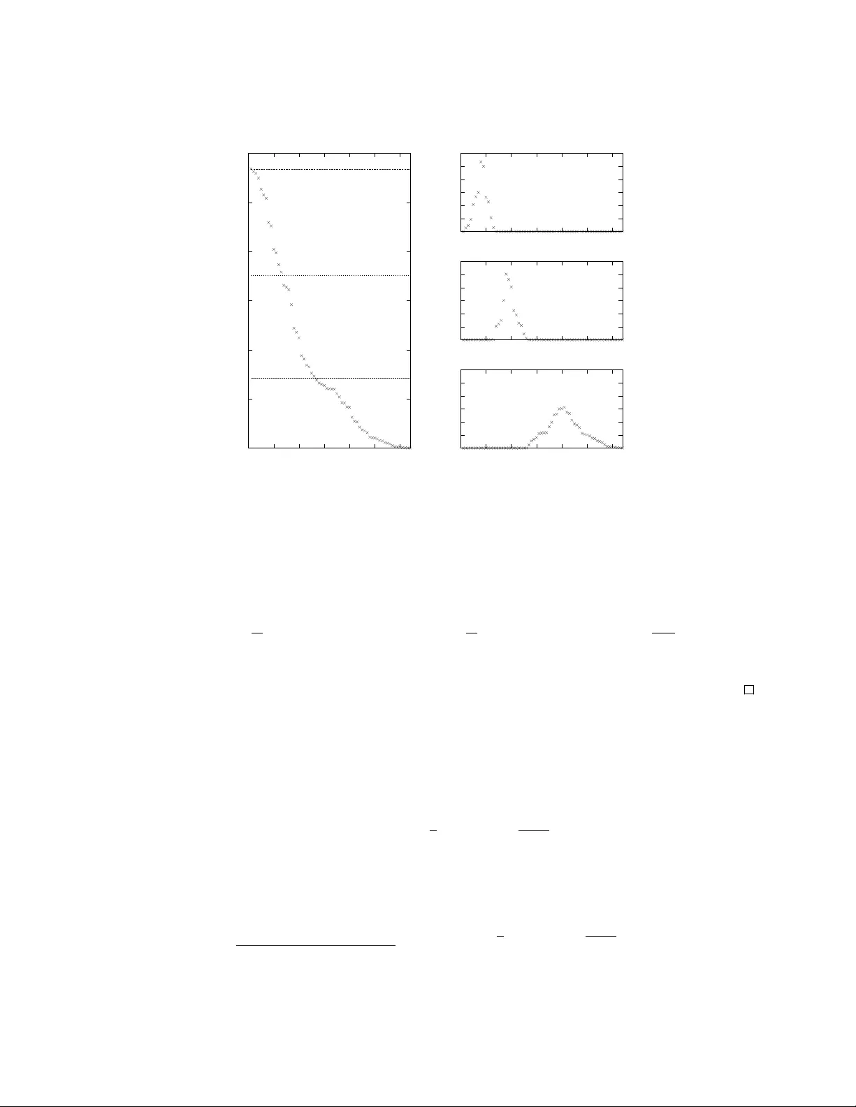
Impro v ed Cheeger’s Inequalit y: Analysis of Sp ectral P artitioning Algorithms through Higher Order Sp ectral Gap Tsz Chiu Kw ok ∗ Lap Chi Lau † Yin T at Lee ‡ Sha yan Ov eis Gharan § Luca T revisan ¶ Abstract Let φ ( G ) be the minim um conductance of an undirected graph G , and let 0 = λ 1 ≤ λ 2 ≤ . . . ≤ λ n ≤ 2 b e the eigenv alues of the normalized Laplacian matrix of G . W e pro ve that for an y graph G and any k ≥ 2, φ ( G ) = O ( k ) λ 2 √ λ k , and this p erformance guaran tee is ac hieved b y the sp ectral partitioning algorithm. This impro ves Cheeger’s inequality , and the bound is optimal up to a constant factor for any k . Our result shows that the sp ectral partitioning algorithm is a constant factor appro ximation algorithm for finding a sparse cut if λ k is a constant for some constant k . This provides some theoretical justification to its empirical p erformance in image segmentation and clustering problems. W e extend the analysis to other graph partitioning problems, including multi-w a y partition, balanced separator, and maximum cut. ∗ The Chinese Universit y of Hong Kong. Supp orted by Hong Kong RGC grant 2150701. Email: tckwok@cse.cuhk.edu.hk † The Chinese Universit y of Hong Kong. Supp orted by Hong Kong RGC grant 2150701. Email: chi@cse.cuhk.edu.hk ‡ The Chinese Universit y of Hong Kong. Currently a PhD student of MIT. Email: yintat@mit.edu § Department of Management Science and Engineering, Stanford Universit y . Supp orted by a Stanford Graduate F ello wship. Email: shayan@stanford.edu ¶ Department of Computer Science, Stanford Univ ersity . This material is based upon w ork supp orted b y the National Science F oundation under grant No. CCF 1017403. Email: trevisan@stanford.edu 1 Con ten ts 1 In tro duction 3 1.1 The Sp ectral Partitioning Algorithm . . . . . . . . . . . . . . . . . . . . . . . . . . . . . . . . 3 1.2 Generalizations of Cheeger’s Inequality . . . . . . . . . . . . . . . . . . . . . . . . . . . . . . . 4 1.3 Analysis of Practical Instances . . . . . . . . . . . . . . . . . . . . . . . . . . . . . . . . . . . 5 1.4 Other Graph Partitioning Problems . . . . . . . . . . . . . . . . . . . . . . . . . . . . . . . . 6 1.5 More Related W ork . . . . . . . . . . . . . . . . . . . . . . . . . . . . . . . . . . . . . . . . . . 6 1.6 Pro of Ov erview . . . . . . . . . . . . . . . . . . . . . . . . . . . . . . . . . . . . . . . . . . . . 7 2 Preliminaries 8 2.1 Sp ectral Theory of the W eighted Laplacian . . . . . . . . . . . . . . . . . . . . . . . . . . . . 9 2.2 Cheeger’s Inequality with Dirichlet Boundary Conditions . . . . . . . . . . . . . . . . . . . . 10 2.3 Energy Low er Bound . . . . . . . . . . . . . . . . . . . . . . . . . . . . . . . . . . . . . . . . . 11 3 Analysis of Sp ectral P artitioning 12 3.1 First Pro of . . . . . . . . . . . . . . . . . . . . . . . . . . . . . . . . . . . . . . . . . . . . . . 12 3.2 Second Pro of . . . . . . . . . . . . . . . . . . . . . . . . . . . . . . . . . . . . . . . . . . . . . 17 4 Extensions and Connections 20 4.1 Sp ectral Multiw ay Partitioning . . . . . . . . . . . . . . . . . . . . . . . . . . . . . . . . . . . 20 4.2 Balanced Separator . . . . . . . . . . . . . . . . . . . . . . . . . . . . . . . . . . . . . . . . . . 22 4.3 Maxim um Cut . . . . . . . . . . . . . . . . . . . . . . . . . . . . . . . . . . . . . . . . . . . . 25 4.3.1 Improv ed Bounds on Bipartiteness Ratio . . . . . . . . . . . . . . . . . . . . . . . . . 26 4.3.2 Improv ed Sp ectral Algorithm for Maximum Cut . . . . . . . . . . . . . . . . . . . . . 28 4.4 Manifold Setting . . . . . . . . . . . . . . . . . . . . . . . . . . . . . . . . . . . . . . . . . . . 32 4.5 Plan ted and Semi-Random Instances . . . . . . . . . . . . . . . . . . . . . . . . . . . . . . . . 32 4.6 Stable Instances . . . . . . . . . . . . . . . . . . . . . . . . . . . . . . . . . . . . . . . . . . . 34 A A New Proof of Cheeger’s Inequalit y 37 B A Differen t Pro of of Theorem 1.2 38 2 1 In tro duction W e study the p erformance of sp ectral algorithms for graph partitioning problems. F or the moment, we assume the graphs are unw eigh ted and d -regular for simplicit y , while the results in the pap er hold for arbitrary w eighted graphs, with suitable c hanges to the definitions. Let G = ( V , E ) be a d -regular undirected graph. The c onductanc e of a subset S ⊆ V is defined as φ ( S ) = | E ( S, S ) | d min {| S | , | S |} , where E ( S, S ) denotes the set of edges of G crossing from S to its complement. The conductance of the graph G is defined as φ ( G ) = min S ⊂ V φ ( S ) . Finding a set of small conductance, also called a sparse cut, is an algorithmic problem that comes up in different areas of computer science. Some applications include image segmen tation [ SM00 , TM06 ], clustering [ NJW01 , KVV04 , Lux07 ], comm unity detection [ LLM10 ], and designing appro ximation algo- rithms [ Shm97 ]. A fundamen tal result in sp ectral graph theory pro vides a connection b et ween the conductance of a graph and the second eigenv alue of its normalized Laplacian matrix. The normalized Laplacian matrix L ∈ R V × V is defined as L = I − 1 d A , where A is the adjacency matrix of G . The eigenv alues of L satisfy 0 = λ 1 ≤ λ 2 ≤ . . . ≤ λ | V | ≤ 2. It is a basic fact that φ ( G ) = 0 if and only if λ 2 = 0. Cheeger’s inequalit y for graphs pro vides a quantitativ e ge neralization of this fact: 1 2 λ 2 ≤ φ ( G ) ≤ p 2 λ 2 . (1.1) This is first prov ed in the manifold setting by Cheeger [ Che70 ] and is extended to undirected graphs b y Alon and Milman [ AM85 , Alo86 ]. Cheeger’s inequalit y is an influential result in sp ectral graph theory with applications in spectral clustering [ ST07 , KVV04 ], explicit construction of expander graphs [ JM85 , HL W06 , Lee12 ], approximate counting [ SJ89 , JSV04 ], and image segmentation [ SM00 ]. W e impro ve Cheeger’s inequality using higher eigenv alues of the normalized Laplacian matrix. Theorem 1.1. F or every undir e cte d gr aph G and any k ≥ 2 , it holds that φ ( G ) = O ( k ) λ 2 √ λ k . This impro ves Cheeger’s inequality , as it sho ws that λ 2 is a b etter approximation of φ ( G ) when there is a large gap b et ween λ 2 and λ k for any k ≥ 3. The b ound is optimal up to a constant factor for any k ≥ 2, as the cycle example shows that φ ( G ) = Ω( k λ 2 / √ λ k ) for any k ≥ 2. 1.1 The Sp ectral Partitioning Algorithm The pro of of Cheeger’s inequalit y is constructiv e and it giv es the follo wing simple nearly-linear time algorithm (the sp e ctr al p artitioning algorithm ) that finds cuts with approximately minimal conductance. Compute the second eigenfunction g ∈ R V of the normalized Laplacian matrix L , and let f = g / √ d . F or a threshold t ∈ R , let V ( t ) := { v : f ( v ) ≥ t } be a threshold set of f . Return the threshold set of f with the minim um conductance among all thresholds t . Let φ ( f ) denote the conductance of the return set of the algorithm. The pro of of Cheeger’s inequality sho ws that 1 2 λ 2 ≤ φ ( f ) ≤ √ 2 λ 2 , and hence the sp ectral partitioning algorithm 3 is a nearly-linear time O (1 / √ λ 2 )-appro ximation algorithm for finding a sparse cut. In particular, it gives a constan t factor approximation algorithm when λ 2 is a constan t, but since λ 2 could be as small as 1 /n 2 ev en for a simple unw eighted graph (e.g. for the cycle), the p erformance guarantee could b e Ω( n ). W e pro ve Theorem 1.1 by sho wing a stronger statement, that is φ ( f ) is upp er-bounded by O ( k λ 2 / √ λ k ). Theorem 1.2. F or any undir e cte d gr aph G , and k ≥ 2 , φ ( f ) = O ( k ) λ 2 √ λ k . This shows that the sp ectral partitioning algorithm is a O ( k / √ λ k )-appro ximation algorithm for the sparsest cut problem, even though it do es not employ any information ab out higher eigen v alues. In particular, sp ectral partitioning provides a constant factor approximation for the sparsest cut problem when λ k is a constan t for some constant k . 1.2 Generalizations of Cheeger’s Inequalit y There are several recent results sho wing new connections b etw een the expansion profile of a graph and the higher eigenv alues of its normalized Laplacian matrix. The first result in this direction is about the small set expansion problem. Arora, Barak and Steurer [ ABS10 ] sho w that if there are k small eigenv alues for some large k , then the graph has a sparse cut S with | S | ≈ n/k . In particular, if k = | V |  for  ∈ (0 , 1), then the graph has a sparse cut S with φ ( S ) ≤ O ( √ λ k ) and | S | ≈ n/k . This can b e seen as a generalization of Cheeger’s inequality to the small set expansion problem (see [ Ste10 , OT12 , OW12 ] for some impro vemen ts). Cheeger’s inequality for graph partitioning can also b e extended to higher-order Cheeger’s inequality for k - w ay graph partitioning [ LR TV12 , LOT12 ]: If there are k small eigenv alues, then there are k disjoin t sparse cuts. Let φ k ( G ) := min S 1 ,...,S k max 1 ≤ i ≤ k φ ( S i ) where S 1 , . . . , S k are ov er non-empty disjoint subsets S 1 , . . . , S k ⊆ V . Then 1 2 λ k ≤ φ k ( G ) ≤ O ( k 2 ) p λ k . Our result can b e applied to k -wa y graph partitioning by com bining with a result in [ LOT12 ]. Corollary 1.3. F or every undir e cte d gr aph G and any l > k ≥ 2 , it holds that (i) φ k ( G ) ≤ O ( lk 6 ) λ k √ λ l . (ii) F or any δ ∈ (0 , 1) , φ (1 − δ ) k ( G ) ≤ O  l log 2 k δ 8 k  λ k √ λ l . (iii) If G excludes K h as a minor, then for any δ ∈ (0 , 1) φ (1 − δ ) k ( G ) ≤ O  h 4 l δ 5 k  λ k √ λ l . 4 P art (i) sho ws that λ k is a b etter appro ximation of φ k ( G ) when there is a large gap b et ween λ k and λ l for any l > k . P art (ii) implies that φ 0 . 9 k ( G ) ≤ O ( λ k log 2 k / √ λ 2 k ), and similarly part (iii) implies that φ 0 . 9 k ( G ) ≤ O ( λ k / √ λ 2 k ) for planar graphs. F urthermore, our pro of shows that the spectral algorithms in [ LOT12 ] ac hieve the corresponding approxima- tion factors. F or instance, when λ l is a constant for a constan t l > k , there is a constan t factor appro ximation algorithm for the k -wa y partitioning problem. 1.3 Analysis of Practical Instances Sp ectral partitioning is a p opular heuristic in practice, as it is easy to b e implemen ted and can b e solv ed efficien tly b y standard linear algebra methods. Also, it has goo d empirical p erformance in applications including image segmentation [ SM00 ] and clustering [ Lux07 ], m uch b etter than the worst case p erformance guaran tee provided by Cheeger’s inequality . It has b een an open problem to explain this phenomenon rigorously [ ST07 , GM98 ]. There are some research directions tow ards this ob jective. One direction is to analyze the a v erage case performance of sp ectral partitioning. A well-studied mo del is the random planted mo del [ Bop87 , AKS98 , McS01 ], where there is a hidden bisection ( X, Y ) of V and there is an edge b etw een t wo v ertices in X and t wo v ertices in Y with probabilit y p and there is an edge b et ween a vertex in X and a v ertex in Y with probability q . It is prov ed that sp ectral techniques can be used to reco ver the hidden partition with high probability , as long as p − q ≥ Ω( p p log | V | / | V | ) [ Bop87 , McS01 ]. The sp ectral approach can also b e used for other hidden graph partitioning problems [ AKS98 , McS01 ]. Note that the spectral algorithms used are usually not exactly the same as the sp ectral partitioning algorithm. Some of these pro ofs explicitly or implicitly use the fact that there is a gap b et ween the second and the third eigen v alues. See Subsection 4.5 for more details. T o b etter mo del practical instances, Bilu and Linial [ BL10 ] in tro duced the notion of stable instances for clustering problems. One definition for the sparsest cut problem is as follo ws: an instance is said to b e γ -stable if there is an optimal sparse cut S ⊆ V whic h will remain optimal even if the weigh t of each edge is p erturbed by a factor of γ . Intuitiv ely this notion is to capture the instances with an outstanding solution that is stable under noise, and arguably they are the meaningful instances in practice. Note that a planted bisection instance is stable if p − q is large enough, and so this is a more general mo del than the planted random mo del. Several clustering problems are shown to b e easier on s table instances [ BBG09 , ABS10 , DLS12 ], and spectral techniques hav e b een analyzed for the stable maximum cut problem [ BL10 , BDLS12 ]. See Subsection 4.6 for more details. Informally , the higher order Cheeger’s inequalit y shows that an undirected graph has k disjoin t sparse cuts if and only if λ k is small. This suggests that the graph has at most k − 1 outstanding sparse cuts when λ k − 1 is small and λ k is large. The algebraic condition that λ 2 is small and λ 3 is large seems similar to the stabilit y condition but more adaptable to spectral analysis. This motiv ates us to analyze the p erformance of the sp ectral partitioning algorithm through higher-order sp ectral gaps. In practical instances of image segmentation, there are usually only a few outstanding ob jects in the image, and so λ k is large for a small k [ Lux07 ]. Thus Theorem 1.2 pro vides a theoretical explanation to why the sp ectral partitioning algorithm performs m uch b etter than the worst case bound b y Cheeger’s inequality in those instances. In clustering applications, there is a well-kno wn eigengap heuristic that partitions the data into k clusters if λ k is small and λ k +1 is large [ Lux07 ]. Corollary 1.3 shows that in such situations the spectral algorithms in [ LOT12 ] p erform b etter than the w orst case b ound by the higher order Cheeger’s inequalit y . 5 1.4 Other Graph P artitioning Problems Our techniques can b e used to improv e the sp ectral algorithms for other graph partitioning problems using higher order eigenv alues. In the minim um bisection problem, the ob jective is to find a set S with minimum conductance among the sets with | V | / 2 v ertices. While it is v ery non trivial to find a sparse cut with exactly | V | / 2 v ertices [ FK02 , Rac08 ], it is well known that a simple recursive sp ectral algorithm can find a b alanc e d sep ar ator S with φ ( S ) = O ( √  ) with | S | = Ω( | V | ), where  denotes the conductance of the minimum bisection (e.g. [ KVV04 ]). W e use Theorem 1.2 to generalize the recursiv e sp ectral algorithm to obtain a b etter appro ximation guarantee when λ k is large for a small k . Theorem 1.4. L et  := min | S | = | V | / 2 φ ( S ) . Ther e is a p olynomial time algorithm that finds a set S such that | V | / 5 ≤ | S | ≤ 4 | V | / 5 and φ ( S ) ≤ O ( k /λ k ) . In the maximum cut problem, the ob jective is to find a partition of the v ertices whic h maximizes the weigh t of edges whose endp oin ts are on different sides of the partition. Go emans and Williamson [ GW95 ] gav e an SDP-based 0 . 878-appro ximation algorithm for the maximum cut problem. T revisan [ T re09 ] gav e a sp ectral algorithm with appro ximation ratio strictly better than 1 / 2. Both algorithms find a solution that cuts at least 1 − O ( √  ) fraction of edges when the optimal solution cuts at least 1 − O (  ) fraction of edges. Using a similar metho d as in the pro of of Theorem 1.2 , we generalize the sp ectral algorithm in [ T re09 ] for the maxim um cut problem to obtain a b etter appro ximation guaran tee when λ n − k is small for a small k . Theorem 1.5. Ther e is a p olynomial time algorithm that on input gr aph G finds a cut ( S, S ) such that if the optimal solution cuts at le ast 1 −  fr action of the e dges, then ( S, S ) cuts at le ast 1 − O ( k ) log  2 − λ n − k k    2 − λ n − k fr action of e dges. 1.5 More Related W ork Appr oximating Gr aph Partitioning Pr oblems: Besides sp ectral partitioning, there are approximation algo- rithms for the sparsest cut problem based on linear and semidefinite programming relaxations. There is an LP-based O (log n ) appro ximation algorithm by Leighton and Rao [ LR99 ], and an SDP-based O ( √ log n ) ap- pro ximation algorithm b y Arora, Rao and V azirani [ AR V04 ]. The subspace en umeration algorithm b y Arora, Barak and Steurer [ ABS10 ] pro vides an O (1 /λ k ) approximation algorithm for the sparsest cut problem with running time n O ( k ) , by searc hing for a sparse cut in the ( k − 1)-dimensional eigenspace corresp onding to λ 1 , . . . , λ k − 1 . It is w orth noting that for k = 3 the subspace en umeration algorithm is exactly the same as the sp ectral partitioning algorithm. Nonetheless, the result in [ ABS10 ] is incomparable to Theorem 1.2 since it do es not upp er-bound φ ( G ) by a function of λ 2 and λ 3 . Recently , using the Lasserre hierarch y for SDP relaxations, Guruswami and Sinop [ GS12 ] gav e an O (1 /λ k ) approximation algorithm for the sparsest cut problem with running time n O (1) 2 O ( k ) . Moreov er, the general framework of Guruswami and Sinop [ GS12 ] applies to other graph partitioning problems including minimum bisection and maxim um cut, obtaining appro ximation algorithms with similar p erformance guaran tees and running times. This line of recent work is closely related to ours in the sense that it sho ws that man y graph partitioning problems are easier to appro ximate on graphs with fast gro wing spectrums, i.e. λ k is large for a small k . Although their results giv e muc h b etter approximation guaran tees when k is large, our results show that simple sp ectral algorithms pro vide nontrivial performance guarantees. 6 Higher Eigenvalues of Sp e cial Gr aphs: Another direction to sho w that sp ectral algorithms w ork w ell is to analyze their p erformance in special graph classes. Spielman and T eng [ ST07 ] show ed that λ 2 = O (1 /n ) for a b ounded degree planar graph and a spectral algorithm can find a separator of size O ( √ n ) in such graphs. This result is extended to b ounded gen us graphs by Kelner [ Kel06 ] and to fixed minor free graphs by Biswal, Lee and Rao [ BLR10 ]. This is further extended to higher eigenv alues by Kelner, Lee, Price and T eng [ KLPT11 ]: λ k = O ( k /n ) for planar graphs, b ounded genus graphs, and fixed minor free graphs when the maximum degree is b ounded. Combining with a higher order Cheeger inequalit y for planar graphs [ LOT12 ], this implies that φ k ( G ) = O ( p k /n ) for b ounded degree planar graphs. W e note that these results giv e mathematical b ounds on the conductances of the resulting partitions, but they do not imply that the approximation guaran tee of Cheeger’s inequality could b e impro ved for these graphs, neither do es our result as these graphs ha ve slowly gro wing sp ectrums. Plante d R andom Instanc es, Semi-R andom Instanc es, and Stable Instanc es: W e hav e discussed some previous w ork on these topics, and we will discuss some relations to our results in Subsection 4.5 and Subsection 4.6 . 1.6 Pro of Overview W e start b y describing an informal in tuition of the pro of of Theorem 1.2 for k = 3, and then we describe ho w this in tuition can b e generalized. F or a function f ∈ R V , let R ( f ) = f T Lf / ( d k f k 2 ) be the Ra yleigh quotien t of f (see ( 2.2 ) of Subsection 2.1 for the definition in general graphs). Let f b e a function that is orthogonal to the constant function and that R ( f ) ≈ λ 2 . Supp ose λ 2 is small and λ 3 is large. Then the higher order Cheeger’s inequalit y implies that there is a partitioning of the graph into t wo sets of small conductance, but in every partitioning in to at least three sets, there is a set of large conductance. So, we exp ect the graph to hav e a sparse cut of which the t wo parts are expanders; see [ T an12 ] for a quantitativ e statemen t. Since R ( f ) is small and f is orthogonal to the constan t function, we exp ect that the v ertices in the same expander hav e similar v alues in f and the av erage v alues of the tw o expanders are far apart. Hence, f is similar to a step function with tw o steps representing a cut, and w e exp ect that R ( f ) ≈ φ ( G ) in this case. Therefore, roughly sp eaking, λ 3  λ 2 implies λ 2 ≈ φ ( G ). Con versely , Theorem 1.2 shows that if λ 2 ≈ φ 2 ( G ) then λ 3 ≈ λ 2 . One wa y to pro ve that λ 2 ≈ λ 3 is to find a function f 0 of Rayleigh quotien t close to λ 2 suc h that f 0 is orthogonal to b oth f and the constant function. F or example, if G is a cycle, then λ 2 = Θ(1 /n 2 ), φ ( G ) = Θ(1 /n ), and f (up to normalizing factors) could represen t the cosine function. In this case we may define f 0 to b e the sine function. Unfortunately , finding suc h a function f 0 in general is not as straightforw ard. Instead, our idea is to find three disjointly supp orte d functions f 1 , f 2 , f 3 of Rayleigh quotien t close to λ 2 . As we prov e in Lemma 2.3 , this would upper-b ound λ 3 b y 2 max {R ( f 1 ) , R ( f 2 ) , R ( f 3 ) } . F or the cycle example, if f is the cosine function, we may construct f 1 , f 2 , f 3 simply b y first dividing the support of f in to three disjoint interv als and then constructing eac h f i b y defining a smooth lo calization of f in one of those interv als. T o ensure that max {R ( f 1 ) , R ( f 2 ) , R ( f 3 ) } ≈ λ 2 w e need to show that f is a “smo oth” function, whose v alues change contin uously . W e make this rigorous by showing that if λ 2 ≈ φ ( G ) 2 , then the function f must b e smooth. Therefore, we can construct three disjointly supp orted functions based on f and show that λ 2 ≈ λ 3 . W e provide t wo proofs of Theorem 1.2 . The first pro of generalizes the first observ ation. W e show that if λ k  k λ 2 , then φ ( G ) ≈ k λ 2 . The main idea is to sho w that if λ k  k λ 2 , then f can b e approximated by a k step function g in the sense that k f − g k ≈ 0 (in general we show that any function f can b e appro ximated b y a k step function g suc h that any k f − g k 2 ≤ R ( f ) /λ k ). It is instructive to pro v e that if f is exactly a k -step function then φ ( G ) ≤ O ( k R ( f )). Our main technical step, Prop osition 3.2 , provides a robust version of the latter fact b y sho wing that for an y k -step approximation of f , φ ( f ) ≤ O ( k ( R ( f ) + k f − g k p R ( f ))). On the other hand, our second pro of generalizes the second observ ation. Say R ( f ) ≈ φ ( G ) 2 . W e partition the support of f in to disjoin t in terv als of the form [2 − i , 2 − ( i +1) ], and we show that the v ertices are distributed 7 almost uniformly in most of these in terv als in the sense that if w e divide [2 − i , 2 − ( i +1) ] in to k equal length subin terv als, then we expect to see the same amount of mass in the subinterv als. This shows that f is a smo oth function. W e then argue that λ k . kλ 2 , by constructing k disjointly supported functions each of Ra yleigh quotient O ( k 2 ) R ( f ). 2 Preliminaries Let G = ( V , E , w ) be a finite, undirected graph, with p ositive w eights w : E → (0 , ∞ ) on the edges. F or a pair of vertices u, v ∈ V , w e write w ( u, v ) for w ( { u, v } ). F or a subset of vertices S ⊆ V , w e write E ( S ) := {{ u, v } ∈ E : u, v ∈ S } . F or disjoint sets S , T ⊆ V , w e write E ( S, T ) := {{ u, v } ∈ E : u ∈ S, v ∈ T } . F or a subset of edges F ⊆ E , we write w ( F ) = P e ∈ F w ( e ). W e use u ∼ v to denote { u, v } ∈ E . W e extend the w eight to vertices by defining, for a single vertex v ∈ V , w ( v ) := P u ∼ v w ( u, v ). W e can think of w ( v ) as the weigh ted degree of vertex v . F or the sake of clarity we will assume throughout that w ( v ) ≥ 1 for every v ∈ V . F or S ⊆ V , w e write vol( S ) = P v ∈ S w ( v ) to denote the volume of S . Giv en a subset S ⊆ V , w e denote the Dirichlet c onductanc e of S by φ ( S ) := w ( E ( S, S )) min { v ol( S ) , vol( S ) } . F or a function f ∈ R V , and a threshold t ∈ R , let V f ( t ) := { v : f ( v ) ≥ t } b e a threshold set of f . W e le t φ ( f ) := min t ∈ R φ ( V f ( t )) . b e the conductance of the b est threshold set of the function f , and V f ( t opt ) b e the smaller side (in v olume) of that minimum cut. F or an y tw o thresholds t 1 , t 2 ∈ R , we use [ t 1 , t 2 ] := { x ∈ R : min { t 1 , t 2 } < x ≤ max { t 1 , t 2 }} . Note that all interv als are defined to b e closed on the larger v alue and open on the smaller v alue. F or an in terv al I = [ t 1 , t 2 ] ⊆ R , we use len( I ) := | t 1 − t 2 | to denote the length of I . F or a function f ∈ R V , we define V f ( I ) := { v : f ( v ) ∈ I } to denote the vertices within I . The volume of an in terv al I is defined as v ol f ( I ) := v ol( V f ( I )). W e also abuse the notation and use v ol f ( t ) := v ol( V f ( t )) to denote the volume of the in terv al [ t, ∞ ]. W e define the supp ort of f , supp( f ) := { v : f ( v ) 6 = 0 } , as the set of vertices with nonzero v alues in f . W e say tw o functions f , g ∈ R V are disjointly supp orted if supp( f ) ∩ supp( g ) = ∅ . F or an y t 1 , t 2 , . . . , t l ∈ R , let ψ : R → R b e defined as ψ t 1 ,...,t l ( x ) = argmin t i | x − t i | . In words, for any x ∈ R , ψ t 1 ,...,t i ( x ) is the v alue of t i closest to x . F or ρ > 0, we sa y a function g is ρ -Lipschitz w.r.t. f , if for all pairs of v ertices u, v ∈ V , | g ( u ) − g ( v ) | ≤ ρ | f ( u ) − f ( v ) | . The next inequalit y follo ws from the Cauc hy-Sc hw arz inequality and will b e useful in our pro of. Let a 1 , . . . , a m , b 1 , . . . , b m ≥ 0. Then, m X i =1 a 2 i b i ≥ ( P m i =1 a i ) 2 P m i =1 b i . (2.1) 8 2.1 Sp ectral Theory of the W eigh ted Laplacian W e write ` 2 ( V , w ) for the Hilb ert space of functions f : V → R with inner pro duct h f , g i w := X v ∈ V w ( v ) f ( v ) g ( v ) , and norm k f k 2 w = h f , f i w . W e reserve h· , ·i and k · k for the standard inner pro duct and norm on R k , k ∈ N and ` 2 ( V ). W e consider some op erators on ` 2 ( V , w ). The adjacency op erator is defined by Af ( v ) = P u ∼ v w ( u, v ) f ( u ), and the diagonal degree op erator by D f ( v ) = w ( v ) f ( v ). Then the c ombinatorial L aplacian is defined by L = D − A , and the normalize d L aplacian is given b y L G := I − D − 1 / 2 AD − 1 / 2 . Observ e that for a d -regular unw eigh ted graph, we hav e L G = 1 d L . If g : V → R is a non-zero function and f = D − 1 / 2 g , then h g , L G g i h g , g i = h g , D − 1 / 2 LD − 1 / 2 g i h g , g i = h f , Lf i h D 1 / 2 f , D 1 / 2 f i = X u ∼ v w ( u, v ) | f ( u ) − f ( v ) | 2 k f k 2 w =: R G ( f ) (2.2) where the latter v alue is referred to as the R ayleigh quotient of f (with r esp e ct to G ) . W e drop the subscript of R G ( f ) when the graph is clear in the context. In particular, L G is a p ositiv e-definite op erator with eigenv alues 0 = λ 1 ≤ λ 2 ≤ · · · ≤ λ n ≤ 2 . F or a connected graph, the first eigen v alue corresp onds to the eigenfunction g = D 1 / 2 f , where f is any non-zero constant function. F urthermore, b y standard v ariational principles, λ k = min g 1 ,...,g k ∈ ` 2 ( V ) max g 6 =0  h g , L G g i h g , g i : g ∈ span { g 1 , . . . , g k }  = min f 1 ,...,f k ∈ ` 2 ( V ,w ) max f 6 =0 n R ( f ) : f ∈ span { f 1 , . . . , f k } o , (2.3) where b oth minimums are o ver sets of k non-zero orthogonal functions in the Hilb ert spaces ` 2 ( V ) and ` 2 ( V , w ), resp ectiv ely . W e refer to [ Chu97 ] for more bac kground on the sp ectral theory of the normalized Laplacian. The following proposition is pro ved in [ HL W06 ] and will b e useful in our pro of Prop osition 2.1 (Horry , Linial and Widgerson [ HL W06 ]) . Ther e ar e two disjointly supp orte d functions f + , f − ∈ ` 2 ( V , w ) such that f + ≥ 0 and f − ≤ 0 and R ( f + ) ≤ λ 2 and R ( f − ) ≤ λ 2 . Pr o of. Let g ∈ ` 2 ( V ) b e the second eigenfunction of L . Let g + ∈ ` 2 ( V ) b e the function with g + ( u ) = max { g ( u ) , 0 } and g − ∈ ` 2 ( V ) be the function with g − ( u ) = min { g ( u ) , 0 } . Then, for an y v ertex u ∈ supp( g + ), ( L g + )( u ) = g + ( u ) − X v : v ∼ u w ( u, v ) g + ( v ) p w ( u ) w ( v ) ≤ g ( u ) − X v : v ∼ u w ( u, v ) g ( v ) p w ( u ) w ( v ) = ( L g )( u ) = λ 2 · g ( u ) . Therefore, h g + , L g + i = X u ∈ supp( g + ) g + ( u ) · ( L g + )( u ) ≤ X u ∈ supp( g + ) λ 2 · g + ( u ) 2 = λ 2 · k g + k 2 . 9 Letting f + = D − 1 / 2 g + , we get λ 2 ≥ h g + , L g + i k g + k 2 = h f + , Lf + i k f + k 2 w = R ( f + ) . Similarly , w e can define f − = D − 1 / 2 g − , and show that R ( f − ) ≤ λ 2 . By c ho osing either of f + or f − that has a smaller (in volume) supp ort, and taking a prop er normalization, w e get the following corollary . Corollary 2.2. Ther e exists a function f ∈ ` 2 ( V , w ) such that f ≥ 0 , R ( f ) ≤ λ 2 , supp( f ) ≤ vol( V ) / 2 , and k f k w = 1 . Instead of directly upp er b ounding λ k in the pro of of Theorem 1.2 , we will construct k disjointly supported functions with small Rayleigh quotients. In the next lemma w e show that b y the v ariational principle this giv es an upp er-b ound on λ k . Lemma 2.3. F or any k disjointly supp orte d functions f 1 , f 2 , . . . , f k ∈ ` 2 ( V , w ) , we have λ k ≤ 2 max 1 ≤ i ≤ k R ( f i ) . Pr o of. By equation ( 2.3 ), it is sufficient to show that for any function h ∈ span { f 1 , . . . , f k } , R ( h ) ≤ max i R ( f i ). Note that R ( f i ) = R ( cf i ) for an y constant c , so we can assume h := P k i =1 f i . Since f 1 , . . . , f k are disjointly supp orted, for any u, v ∈ V , we hav e | h ( u ) − h ( v ) | 2 ≤ k X i =1 2 | f i ( u ) − f i ( v ) | 2 . Therefore, R ( h ) = P u ∼ v w ( u, v ) | h ( u ) − h ( v ) | 2 k h k 2 w ≤ 2 P u ∼ v P k i =1 w ( u, v ) | f i ( u ) − f i ( v ) | 2 k h k 2 w = 2 P k i =1 P u ∼ v w ( u, v ) | f i ( u ) − f i ( v ) | 2 P k i =1 k f i k 2 w ≤ 2 max 1 ≤ i ≤ k R ( f i ) . 2.2 Cheeger’s Inequalit y with Diric hlet Boundary Conditions Man y v ariants of the following lemma are kno wn; see, e.g. [ Chu96 ]. Lemma 2.4. F or every non-ne gative h ∈ ` 2 ( V , w ) such that supp( h ) ≤ vol( V ) / 2 , the fol lowing holds φ ( h ) ≤ P u ∼ v w ( u, v ) | h ( v ) − h ( u ) | P v w ( v ) h ( v ) . Pr o of. Since the right hand side is homogeneous in h , we may assume that max v h ( v ) ≤ 1. Let 0 < t ≤ 1 b e c hosen uniformly at random. Then, by linearity of exp ectation, E h w ( E ( V h ( t ) , V h ( t ))) i E [vol( V h ( t ))] = P u ∼ v w ( u, v ) | h ( u ) − h ( v ) | P v w ( v ) h ( v ) . 10 This implies that there exists a 0 < t ≤ 1 such that φ ( V h ( t )) ≤ P u ∼ v w ( u,v ) | h ( v ) − h ( u ) | P v w ( v ) h ( v ) . The latter holds since for any t > 0, vol( V h ( t )) ≤ vol( V ) / 2. 2.3 Energy Lo w er Bound W e define the ener gy of a function f ∈ ` 2 ( V , w ) as E f := X u ∼ v w ( u, v ) | f ( u ) − f ( v ) | 2 . Observ e that R ( f ) = E f / k f k 2 w . W e also define the energy of f r estricte d to an interv al I as follows: E f ( I ) := X u ∼ v w ( u, v ) len( I ∩ [ f ( u ) , f ( v )]) 2 . When the function f is clear from the context w e drop the subscripts from the ab o v e definitions. The next fact shows that by restricting the energy of f to disjoint in terv als w e may only decrease the energy . F act 2.5. F or any set of disjoint intervals I 1 , . . . , I m , we have E f ≥ m X i =1 E f ( I i ) . Pr o of. E f = X u ∼ v w ( u, v ) | f ( u ) − f ( v ) | 2 ≥ X u ∼ v m X i =1 w ( u, v ) len( I i ∩ [ f ( u ) , f ( v )]) 2 = m X i =1 E f ( I i ) . The following is the k ey lemma to low er b ound the energy of a function f . It shows that a long interv al with small volume must ha ve a significant con tribution to the energy of f . Lemma 2.6. F or any non-ne gative function f ∈ ` 2 ( V , w ) with v ol(supp( f )) ≤ v ol( V ) / 2 , for any interval I = [ a, b ] with a > b ≥ 0 , we have E ( I ) ≥ φ 2 ( f ) · v ol 2 f ( a ) · len 2 ( I ) φ ( f ) · v ol f ( a ) + v ol f ( I ) . Pr o of. Since f is non-negativ e with v ol(supp( f )) ≤ vol( V ) / 2, by the definition of φ ( f ), the total weigh t of the edges going out the threshold set V f ( t ) is at least φ ( f ) · vol f ( a ), for any a ≥ t ≥ b ≥ 0. Therefore, b y summing ov er these threshold sets, we ha ve X u ∼ v w ( u, v ) len( I ∩ [ f ( u ) , f ( v )]) ≥ len( I ) · φ ( f ) · vol f ( a ) . Let E 0 := {{ u, v } : len( I ∩ [ f ( u ) , f ( v )]) > 0 } b e the set of edges with nonempty intersection with the in terv al I . Let β ∈ (0 , 1) be a parameter to b e fixed later. Let F ⊆ E 0 b e the set of edges of E 0 that are not adjacent to any of the vertices in I . If w ( F ) ≥ β w ( E 0 ), then E ( I ) ≥ w ( F ) · len( I ) 2 ≥ β · w ( E 0 ) · len( I ) 2 ≥ β · φ ( f ) · v ol f ( a ) · len( I ) 2 . 11 Otherwise, vol f ( I ) ≥ (1 − β ) w ( E 0 ). Therefore, by the Cauch y Sch warz inequalit y ( 2.1 ), we ha ve E ( I ) = X { u,v }∈ E 0 w ( u, v )(len( I ∩ [ f ( u ) , f ( v )])) 2 ≥  P { u,v }∈ E 0 w ( u, v ) len( I ∩ [ f ( u ) , f ( v )])  2 w ( E 0 ) ≥ (1 − β ) len( I ) 2 · φ ( f ) 2 · v ol 2 f ( a ) v ol f ( I ) . Cho osing β = ( φ ( f ) · vol f ( a )) / ( φ ( f ) · v ol f ( a ) + v ol f ( I )) such that the ab o ve tw o terms are equal giv es the lemma. W e note that Lemma 2.6 can be used to give a new pro of of Cheeger’s inequalit y with a w eaker constant; see App endix A . 3 Analysis of Sp ectral P artitioning Throughout this section we assume that f ∈ ` 2 ( V , w ) is a non-negative function of norm k f k 2 w = 1 such that R ( f ) ≤ λ 2 and v ol(supp( f )) ≤ v ol( V ) / 2. The existence of this function follows from Corollary 2.2 . In Subsection 3.1 , w e giv e our first pro of of Theorem 1.2 which is based on the idea of appro ximating f by a 2 k + 1 step function g . Our second pro of is given in Subsection 3.2 . 3.1 First Pro of W e sa y a function g ∈ ` 2 ( V , w ) is a l -step approximation of f , if there exist l thresholds 0 = t 0 ≤ t 1 ≤ . . . ≤ t l − 1 suc h that for every v ertex v , g ( v ) = ψ t 0 ,t 1 ,...,t l − 1 ( f ( v )) . In words, g ( v ) = t i if t i is the closest threshold to f ( v ); see Figure 3.1 for an example. t i − 1 t i t i +1 Figure 3.1: The crosses denote the v alues of function f , and the circles denote the v alues of function g . W e show that if there is a large gap b et ween λ 2 and λ k , then the function f is well approximated by a step function g with at most 2 k + 1 steps. Then we define an appropriate h and apply Lemma 2.4 to get a low er b ound on the energy of f in terms of k f − g k 2 w . One can think of h as a probability distribution function on the threshold sets, and we will define h in suc h a w ay that the threshold sets that are further aw ay from the thresholds t 0 , t 1 , . . . , t 2 k ha ve higher probability . 12 Appro ximating f by a 2 k + 1 Step F unction In the next lemma we sho w that if there is a large gap betw een R ( f ) and λ k , then there is a 2 k + 1-step function g suc h that k f − g k 2 w = O ( R ( f ) /λ k ). Lemma 3.1. Ther e exists a 2 k + 1 -step appr oximation of f , c al l g , such that k f − g k 2 w ≤ 4 R ( f ) λ k . (3.1) Pr o of. Let M := max v f ( v ). W e will find 2 k + 1 thresholds 0 =: t 0 ≤ t 1 ≤ . . . ≤ t 2 k = M , then we let g b e a 2 k + 1 step approximation of f with these thresholds. Let C := 2 R ( f ) /k λ k . W e choose these thresholds inductiv ely . Giv en t 0 , t 1 , . . . , t i − 1 , we let t i − 1 ≤ t i ≤ M to b e the smallest n umber such that X v : t i − 1 ≤ f ( v ) ≤ t i w ( v ) | f ( v ) − ψ t i − 1 ,t i ( f ( v )) | 2 = C. (3.2) Observ e that the left hand side v aries con tinuously with t i : when t i = t i − 1 the left hand side is zero, and for larger t i it is non-decreasing. If w e can satisfy ( 3.2 ) for some t i − 1 ≤ t i ≤ M , then w e let t i to be the smallest such num b er, and otherwise we set t i = M . W e say the pro cedure suc c e e ds if t 2 k = M . W e will show that: (i) if the pro cedure succeeds then the lemma follo ws, and (ii) that the pro cedure alw ays succeeds. Part (i) is clear b ecause if w e define g to b e the 2 k + 1 step approximation of f with resp ect to t 0 , . . . , t 2 k , then k f − g k 2 w = 2 k X i =1 X v : t i − 1 ≤ f ( v ) ≤ t i w ( v ) | f ( v ) − ψ t i − 1 ,t i ( f ( v )) | 2 ≤ 2 k C = 4 R ( f ) λ k , and we are done. The inequalit y in the ab o ve equation follows b y ( 3.2 ). Supp ose to the contrary that the pro cedure do es not succeed. W e will construct 2 k disjoin tly supp orted functions of Ra yleigh quotients less than λ k / 2, and then use Lemma 2.3 to get a con tradiction. F or 1 ≤ i ≤ 2 k , let f i b e the following function (see Figure 3.2 for an illustration): f i ( v ) :=  | f ( v ) − ψ t i − 1 ,t i ( f ( v )) | if t i − 1 ≤ f ( v ) ≤ t i 0 otherwise . W e will argue that at least k of these functions hav e R ( f i ) < 1 2 λ k . By ( 3.2 ), w e already know that the denominators of R ( f i ) are equal to C ( k f i k 2 w = C ), so it remains to find an upper bound for the numerators. F or an y pair of vertices u, v , we show that 2 k X i =1 | f i ( u ) − f i ( v ) | 2 ≤ | f ( u ) − f ( v ) | 2 . (3.3) The inequality follows using the fact that f 1 , . . . , f 2 k are disjointly supp orted, and th us u, v are con tained in the supp ort of at most tw o of these functions. If b oth u and v are in the supp ort of only one function, then ( 3.3 ) holds since eac h f i is 1-Lipsc hitz w.r.t. f . Otherwise, say u ∈ supp( f i ) and v ∈ supp( f j ) for i < j , then ( 3.3 ) holds since | f i ( u ) − f i ( v ) | 2 + | f j ( u ) − f j ( v ) | 2 = | f ( u ) − g ( u ) | 2 + | f ( v ) − g ( v ) | 2 ≤ | f ( u ) − t i | 2 + | f ( v ) − t i | 2 ≤ | f ( u ) − f ( v ) | 2 . 13 0 0.01 0.02 0.03 0.04 0.05 0.06 0 10 20 30 40 50 60 0 0.01 0.02 0.03 0.04 0.05 0.06 0 10 20 30 40 50 60 0 0.01 0.02 0.03 0.04 0.05 0.06 0 10 20 30 40 50 60 0 0.05 0.1 0.15 0.2 0.25 0.3 0 10 20 30 40 50 60 Figure 3.2: The figure on the left is the function f with k f k w = 1. W e cut f in to three disjointly supp orted v ectors f 1 , f 2 , f 3 b y setting t 0 = 0, t 1 ≈ 0 . 07, t 2 ≈ 0 . 175, and t 3 = max f ( v ). F or each 1 ≤ i ≤ 3, we define f i ( v ) = min {| f ( v ) − t i − 1 | , | f ( v ) − t i |} , if t i − 1 ≤ f ( v ) ≤ t i , and zero otherwise. Summing ( 3.3 ) we hav e 2 k X i =1 R ( f i ) = 1 C 2 k X i =1 X u ∼ v w ( u, v ) | f i ( u ) − f i ( v ) | 2 ≤ 1 C X u ∼ v w ( u, v ) | f ( u ) − f ( v ) | 2 = k λ k 2 . Hence, by an av eraging argumen t, there are k disjoin tly functions f 0 1 , . . . , f 0 k of Rayleigh quotients less than λ k / 2, a contradiction to Lemma 2.3 . Upp er Bounding φ ( f ) Using 2 k + 1 Step Approximation g Next , w e show that we can use any function g that is a 2 k + 1 approximation of f to upp er-bound φ ( f ) in terms of k f − g k w . Prop osition 3.2. F or any 2 k + 1 -step appr oximation of f with k f k w = 1 , c al le d g , φ ( f ) ≤ 4 k R ( f ) + 4 √ 2 k k f − g k w p R ( f ) . Let g b e a 2 k + 1 appro ximation of f with thresholds 0 = t 0 ≤ t 1 ≤ . . . ≤ t 2 k , i.e. g ( v ) := ψ t 0 ,t 1 ,...,t 2 k ( f ( v )). W e will define a function h ∈ ` 2 ( V , w ) such that eac h threshold set of h is also a threshold set of f (in particular supp( h ) = supp( f )), and P u ∼ v w ( u, v ) | h ( v ) − h ( u ) | P v w ( v ) h ( v ) ≤ 4 k R ( f ) + 4 √ 2 k k f − g k w p R ( f ) . (3.4) 14 W e then simply use Lemma 2.4 to prov e Prop osition 3.2 . Let µ : R → R , µ ( x ) := | x − ψ t 0 ,t 1 ,...,t 2 k ( x ) | . Note that | f ( v ) − g ( v ) | = µ ( f ( v )). One can think of µ as a probability density function to sample the threshold sets, where threshold sets that are further aw ay from the thresholds t 0 , t 1 , . . . , t 2 k are giv en higher probabilit y . W e define h as follows: h ( v ) := Z f ( v ) 0 µ ( x ) dx Observ e that the threshold sets of h and the threshold sets of f are the same, as h ( u ) ≥ h ( v ) if and only if f ( u ) ≥ f ( v ). It remains to pro ve ( 3.4 ). W e use the follo wing tw o claims, that bound the denominator and the numerator separately . Claim 3.3. F or every vertex v , h ( v ) ≥ 1 8 k f 2 ( v ) . Pr o of. If f ( v ) = 0, then h ( v ) = 0 and there is nothing to pro ve. Supp ose f ( v ) is in the interv al f ( v ) ∈ [ t i , t i +1 ]. Using the Cauch y-Sch warz inequalit y , f 2 ( v ) = ( i − 1 X j =0 ( t j +1 − t j ) + ( f ( v ) − t i )) 2 ≤ 2 k · ( i − 1 X j =0 ( t j +1 − t j ) 2 + ( f ( v ) − t i ) 2 ) . On the other hand, by the definition of h , h ( v ) = i − 1 X j =0 Z t j +1 t j µ ( x ) dx + Z f ( v ) t i µ ( x ) dx = i − 1 X j =0 1 4 ( t j +1 − t j ) 2 + Z f ( v ) t i µ ( x ) dx ≥ i − 1 X j =0 1 4 ( t j +1 − t j ) 2 + 1 4 ( f ( v ) − t i ) 2 , where the inequality follo ws by the fact that f ( v ) ∈ [ t i , t i +1 ]. And we will b ound the numerator with the following claim. Claim 3.4. F or any p air of vertic es u, v ∈ V , | h ( v ) − h ( u ) | ≤ 1 2 | f ( v ) − f ( u ) | · ( | f ( u ) − g ( u ) | + | f ( v ) − g ( v ) | + | f ( v ) − f ( u ) | ) . Pr o of. By the definition of µ ( . ), for an y x ∈ [ f ( u ) , f ( v )], µ ( x ) ≤ min {| x − g ( u ) | , | x − g ( v ) |} ≤ | x − g ( u ) | + | x − g ( v ) | 2 ≤ 1 2  ( | x − f ( u ) | + | f ( u ) − g ( u ) | ) + ( | x − f ( v ) | + | f ( v ) − g ( v ) | )  = 1 2 ( | f ( u ) − g ( u ) | + | f ( v ) − g ( v ) | + | f ( v ) − f ( u ) | ) , 15 where the third inequality follows b y the triangle inequalit y , and the last equality uses x ∈ [ f ( u ) , f ( v )]. Therefore, h ( v ) − h ( u ) = Z f ( v ) f ( u ) µ ( x ) dx ≤ | f ( v ) − f ( u ) | · max x ∈ [ f ( u ) ,f ( v )] µ ( x ) ≤ 1 2 | f ( v ) − f ( u ) | · ( | f ( u ) − g ( u ) | + | f ( v ) − g ( v ) | + | f ( v ) − f ( u ) | ) . No w we are ready to prov e Prop osition 3.2 . Pr o of of Pr op osition 3.2 . First, by Claim 3.4 , X u ∼ v w ( u, v ) | h ( u ) − h ( v ) | ≤ X u ∼ v 1 2 w ( u, v ) | f ( v ) − f ( u ) | · ( | f ( u ) − g ( u ) | + | f ( v ) − g ( v ) | + | f ( v ) − f ( u ) | ) ≤ 1 2 R ( f ) + 1 2 s X u ∼ v w ( u, v ) | f ( v ) − f ( u ) | 2 s X u ∼ v w ( u, v )( | f ( u ) − g ( u ) | + | f ( v ) − g ( v ) | ) 2 ≤ 1 2 R ( f ) + 1 2 p R ( f ) · s 2 X u ∼ v w ( u, v )( | f ( u ) − g ( u ) | 2 + | f ( v ) − g ( v ) | 2 ) = 1 2 R ( f ) + 1 2 p R ( f ) · q 2 k f − g k 2 w , where the second inequality follows b y the Cauch y-Sch warz inequality . On the other hand, b y Claim 3.3 , X v w ( v ) h ( v ) ≥ 1 8 k X v w ( v ) f 2 ( v ) = 1 8 k k f k 2 w = 1 8 k . Putting ab o ve equations together pro ves ( 3.4 ). Since the threshold sets of h are the same as the threshold sets of f , we hav e φ ( f ) = φ ( h ) and the prop osition follo ws by Lemma 2.4 . No w we are ready to prov e Theorem 1.2 . Pr o of of The or em 1.2 . Let g be as defined in Lemma 3.1 . By Prop osition 3.2 , w e get φ ( f ) ≤ 4 k R ( f ) + 4 √ 2 k k f − g k w p R ( f ) ≤ 4 k R ( f ) + 8 √ 2 k R ( f ) / p λ k ≤ 12 √ 2 k R ( f ) / p λ k . W e provide a differen t pro of of Theorem 1.2 in App endix B b y low er-b ounding E f using a 2 k + 1 appro ximation of f . This pro of uses Lemma 2.6 instead of Lemma 2.4 to prov e the theorem. Remark: Claim 3.4 can b e improv ed to | h ( v ) − h ( u ) | ≤ 1 2 | f ( v ) − f ( u ) | · ( | f ( u ) − g ( u ) | + | f ( v ) − g ( v ) | + 1 2 | f ( v ) − f ( u ) | ) , and thus Theorem 1.2 can b e improv ed to φ ( f ) ≤ 10 √ 2 k R ( f ) / √ λ k . 16 3.2 Second Pro of Instead of directly proving Theorem 1.2 , we use Corollary 2.2 and Lemma 2.3 and prov e a stronger v ersion, as it will b e used later to prov e Corollary 1.3 1 . In particular, instead of directly upp er-bounding λ k , we construct k disjoin tly supp orted functions with small Rayleigh quotien ts. Theorem 3.5. F or any non-ne gative function f ∈ ` 2 ( V , w ) such that supp( f ) ≤ vol( V ) / 2 , and δ := φ 2 ( f ) / R ( f ) , at le ast one of the fol lowing holds i) φ ( f ) ≤ O ( k ) R ( f ); ii) Ther e exist k disjointly supp orte d functions f 1 , f 2 , . . . , f k such that for al l 1 ≤ i ≤ k , supp( f i ) ⊆ supp( f ) and R ( f i ) ≤ O ( k 2 ) R ( f ) /δ. F urthermor e, the supp ort of e ach f i is an interval [ a i , b i ] such that | a i − b i | = Θ(1 /k ) a i . W e will show that if R ( f ) = Θ( φ ( G ) 2 ) (when δ = Θ(1)), then f is a smo oth function of the v ertices, in the sense that in an y in terv al of the form [ t, 2 t ] w e exp ect the v ertices to b e em b edded in equidistance positions. It is instructive to verify this for the second eigen vector of the cycle. Construction of Disjoin tly Supp orted F unctions Using Dense W ell Separated Regions First, we show that Theorem 3.5 follo ws from a construction of 2 k dense w ell separated regions, and in the subsequent parts we construct these regions based on f . A region R is a closed subset of R + . Let ` ( R ) := P v : f ( v ) ∈ R w ( v ) f 2 ( v ). W e say R is W -dense if ` ( R ) ≥ W . F or any x ∈ R + , we define dist( x, R ) := inf y ∈ R | x − y | y . The  -neighb orho o d of a region R is the set of p oin ts at distance at most  from R , N  ( R ) := { x ∈ R + : dist( x, R ) <  } . W e sa y t wo regions R 1 , R 2 are  -wel l-sep ar ate d , if N  ( R 1 ) ∩ N  ( R 2 ) = ∅ . In the next lemma, we show that our main theorem can b e prov ed by finding 2 k , Ω( δ /k )-dense, Ω(1 /k ) well-separated regions. Lemma 3.6. L et R 1 , R 2 , . . . , R 2 k b e a set of W -dense and  -wel l sep ar ate d r e gions. Then, ther e ar e k disjointly supp orte d functions f 1 , . . . , f k , e ach supp orte d on the  -neighb orho o d of one of the r e gions such that ∀ 1 ≤ i ≤ k , R ( f i ) ≤ 2 R ( f ) k  2 W . Pr o of. F or any 1 ≤ i ≤ 2 k , we define a function f i , where for all v ∈ V , f i ( v ) := f ( v ) max { 0 , 1 − dist( f ( v ) , R i ) / } . Then, k f i k 2 w ≥ ` ( R i ). Since the regions are  -w ell separated, the functions are disjointly supp orted. There- fore, the endp oin ts of each edge { u, v } ∈ E are in the support of at most tw o functions. Th us, by an 1 W e note that the first pro of can also b e mo dified to obtain this stronger version, without the additional property that each f i is defined on an interv al [ a i , b i ] of the form | a i − b i | = Θ(1 /k ) a i . See Lemma 4.12 for an adaptation of Lemma 3.1 to pro ve such a statement for maximum cut. 17 a veraging argument, there exist k functions f 1 , f 2 , . . . , f k (ma yb e after renaming) satisfy the following. F or all 1 ≤ i ≤ k , X u ∼ v w ( u, v ) | f i ( u ) − f i ( v ) | 2 ≤ 1 k 2 k X j =1 X u ∼ v w ( u, v ) | f j ( u ) − f j ( v ) | 2 . Therefore, for 1 ≤ i ≤ k , R ( f i ) = P u ∼ v w ( u, v ) | f i ( u ) − f i ( v ) | 2 k f i k 2 w ≤ P 2 k j =1 P u ∼ v w ( u, v ) | f j ( u ) − f j ( v ) | 2 k · min 1 ≤ i ≤ 2 k k f i k 2 w ≤ 2 P u ∼ v w ( u, v ) | f ( u ) − f ( v ) | 2 k  2 W = 2 R ( f ) k  2 W , where we used the fact that f j ’s are 1 / -Lipschitz. Therefore, f 1 , . . . , f k satisfy lemma’s statement. Construction of Dense W ell Separated Regions Let 0 < α < 1 b e a constant that will b e fixed later in the pro of. F or i ∈ Z , we define the interv al I i := [ α i , α i +1 ]. Observ e that these interv als partition the v ertices with positive v alue in f . W e let ` i := ` ( I i ). W e partition each interv al I i in to 12 k subinterv als of equal length, I i,j :=  α i  1 − j (1 − α ) 12 k  , α i  1 − ( j + 1)(1 − α ) 12 k  , for 0 ≤ j < 12 k . Observ e that for all i, j , len( I i,j ) = α i (1 − α ) 12 k . (3.5) Similarly we define ` i,j := ` ( I i,j ). W e say a subinterv al I i,j is he avy , if ` i,j ≥ cδ ` i − 1 /k , where c > 0 is a constan t that will b e fixed later in the proof; we sa y it is light otherwise. W e use H i to denote the set of hea vy subin terv als of I i and L i for the set of ligh t subin terv als. W e use h i to denote the num b er of hea vy subin terv als. W e also say an interv al I i is b alanc e d if h i ≥ 6 k , denoted by I i ∈ B where B is the set of balanced interv als. Intuitiv ely , an interv al I i is b alanc e d if the v ertices are distributed uniformly inside that in terv al. Next w e describ e our pro of strategy . Using Lemma 3.6 to prov e the theorem it is sufficient to find 2 k , Ω( δ /k )- dense, Ω(1 /k ) well-separated regions R 1 , . . . , R 2 k . Each of our 2 k regions will be a union of he avy subin terv als. Our construction is simple: from each balanced in terv al we choose 2 k sep ar ate d hea vy subinterv als and include eac h of them in one of the regions. In order to promise that the regions are well separated, once we include I i,j ∈ H i in to a region R we lea ve the t wo neigh b oring subin terv als I i,j − 1 and I i,j +1 unassigned, so as to separate R from the rest of the regions. In particular, for all 1 ≤ a ≤ 2 k and all I i ∈ B , w e include the (3 a − 1)-th heavy subinterv al of I i in R a . Note that if an interv al I i is balanced, then it has 6 k hea vy subin terv als and we can include one heavy subinterv al in each of the 2 k regions. F urthermore, by ( 3.5 ), the regions are (1 − α ) / 12 k -w ell separated. It remains to pro ve that these 2 k regions are dense. Let ∆ := X I i ∈ B ` i − 1 b e the summation of the mass of the preceding interv al of balanced in terv als. Then, since eac h hea vy subin terv al I i,j has a mass of cδ` i − 1 /k , by the ab o ve construction all regions are c ∆ δ /k -dense. Hence, the follo wing prop osition follows from Lemma 3.6 . 18 Prop osition 3.7. Ther e ar e k disjoint supp orte d functions f 1 , . . . , f k such that for al l 1 ≤ i ≤ k , supp( f i ) ⊆ supp( f ) and ∀ 1 ≤ i ≤ k , R ( f i ) ≤ 300 k 2 R ( f ) (1 − α ) 2 cδ ∆ . Lo wer Bounding the Densit y So in the rest of the pro of we just need to low er-b ound ∆ by an absolute constant. Prop osition 3.8. F or any interval I i / ∈ B , E ( I i ) ≥ α 6 φ ( f ) 2 ` i − 1 (1 − α ) 2 24( k α 4 φ ( f ) + cδ ) . Pr o of. In the next claim, w e low er-b ound the energy of a light subinterv al in terms of ` i − 1 . Then, we prov e the statement simply using h i < 6 k . Claim 3.9. F or any light subinterval I i,j , E ( I i,j ) ≥ α 6 φ ( f ) 2 ` i − 1 (1 − α ) 2 144 k ( kα 4 φ ( f ) + cδ ) . Pr o of. First, observe that ` i − 1 = X v ∈ I i − 1 w ( v ) f 2 ( v ) ≤ α 2 i − 2 v ol( α i ) . (3.6) Therefore, v ol( I i,j ) = X v ∈ I i,j w ( v ) ≤ X v ∈ I i,j w ( v ) f 2 ( v ) α 2 i +2 = ` i,j α 2 i +2 ≤ cδ ` i − 1 k α 2 i +2 ≤ cδ v ol( α i ) k α 4 , (3.7) where w e use the assumption that I i,j ∈ L i in the second last inequality , and ( 3.6 ) in the last inequality . By Lemma 2.6 , E ( I i,j ) ≥ φ ( f ) 2 · v ol( α i ) 2 · len( I i,j ) 2 φ ( f ) · v ol( α i ) + v ol( I i,j ) ≥ k α 4 φ ( f ) 2 · v ol( α i ) · len( I i,j ) 2 k α 4 φ ( f ) + cδ ≥ α 6 φ ( f ) 2 ` i − 1 (1 − α ) 2 144 k ( kα 4 φ ( f ) + cδ ) , where the first inequality holds by ( 3.7 ), and the last inequalit y holds by ( 3.5 ) and ( 3.6 ). No w, since the subinterv als are disjoin t, b y F act 2.5 , E ( I i ) ≥ X I i,j ∈ L i E ( I i,j ) ≥ (12 k − h i ) α 6 φ ( f ) 2 ` i − 1 (1 − α ) 2 144 k ( kφ ( f ) α 4 + cδ ) ≥ α 6 φ ( f ) 2 ` i − 1 (1 − α ) 2 24( k φ ( f ) α 4 + cδ ) , where we used the assumption that I i is not balanced and thus h i < 6 k . No w we are ready to low er-b ound ∆. 19 Pr o of of The or em 3.5 . First w e sho w that ∆ ≥ 1 / 2, unless (i) holds, and then we use Prop osition 3.7 to pro ve the theorem. If φ ( f ) ≤ 10 4 k R ( f ), then (i) holds and we are done. So, assume that 10 8 k 2 R 2 ( f ) φ 2 ( f ) ≤ 1 , (3.8) and we prov e (ii). Since k f k 2 w = 1, by Prop osition 3.8 , R ( f ) = E f ≥ X I i / ∈ B E ( I i ) ≥ X I i / ∈ B α 6 φ ( f ) 2 ` i − 1 (1 − α ) 2 24( k φ ( f ) α 4 + cδ ) . Set α = 1 / 2 and c := α 6 (1 − α ) 2 / 96. If k φ ( f ) α 4 ≥ cδ , then we get X I i / ∈ B ` i − 1 ≤ 48 k R ( f ) α 2 (1 − α ) 2 φ ( f ) ≤ 1 2 , where the last inequality follows from ( 3.8 ). Otherwise, X I i / ∈ B ` i − 1 ≤ 48 cδ R ( f ) α 6 (1 − α ) 2 φ 2 ( f ) ≤ 1 2 , where the last inequality follows from the definition of c and δ . Since ` ( V ) = k f k 2 w = 1, it follows from the ab o v e equations that ∆ ≥ 1 2 . Therefore, by Prop osition 3.7 , w e get k disjointly supp orted functions f 1 , . . . , f k suc h that R ( f i ) ≤ 300 k 2 R ( f ) (1 − α ) 2 cδ ∆ ≤ 10 8 k 2 R ( f ) 2 φ ( f ) 2 . Although each function f i is defined on a region whic h is a union of many hea vy subin terv als, w e can simply restrict it to only one of those subin terv als guaranteeing that R ( f i ) only decreases. Therefore each f i is defined on an interv al [ a i , b i ] where by ( 3.5 ), | a i − b i | = Θ(1 /k ) a i . This prov es (ii). 4 Extensions and Connections In this section, we extend our approac h to other graph partitioning problems, including m ultiwa y partitioning ( Subsection 4.1 ), balanced separator ( Subsection 4.2 ), maxim um cut ( Subsection 4.3 ), and to the manifold setting ( Subsection 4.4 ). Also, we discuss some relations b et ween our setting and the settings for planted and semirandom instances ( Subsection 4.5 ) and in stable instances ( Subsection 4.6 ). 4.1 Sp ectral Multiwa y Partitioning In this subsection, we use Theorem 3.5 and the results in [ LOT12 ] to prov e Corollary 1.3 . Theorem 4.1 ([ LOT12 , Theorem 1.3]) . F or any gr aph G = ( V , E , w ) and any inte ger k , ther e exist k non-ne gative disjointly supp orte d functions f 1 , . . . , f k ∈ ` 2 ( V , w ) such that for e ach 1 ≤ i ≤ k we have R ( f i ) ≤ O ( k 6 ) λ k . 20 Let f 1 , . . . , f k b e as defined ab o ve. W e consider t wo cases. First assume that v ol(supp( f i )) ≤ vol( V ) / 2 for all 1 ≤ i ≤ k . Recall that V f i ( t opt ) is the best threshold set of f i . Let S i := V f i ( t opt ). Then, for eac h function f i , by Theorem 3.5 , φ ( S i ) = φ ( f i ) ≤ O ( l ) R ( f i ) √ λ l ≤ O ( lk 6 ) λ k √ λ l . F urthermore, since S i ⊆ supp( f i ) and f 1 , . . . , f k are disjointly supp orted, S 1 , . . . , S k are disjoint. Hence, φ k ( G ) = max 1 ≤ i ≤ k φ ( S i ) ≤ O ( lk 6 ) λ k √ λ l , and we are done. Now supp ose there exists a function, say f k , with v ol(supp( f k )) > v ol( V ) / 2. Let S i = V f i ( t opt ) for 1 ≤ i ≤ k − 1, and S k := V \ S 1 \ . . . \ S k − 1 . Similar to the abov e, the sets S 1 , . . . , S k − 1 are disjoin t, and φ ( S i ) ≤ O ( lk 6 λ k / √ λ l ) for all 1 ≤ i ≤ k − 1. Observe that φ ( S k ) = w ( E ( S 1 , S k )) + . . . + w ( E ( S k − 1 , S k )) v ol( V ) − v ol( S k ) ≤ P k − 1 i =1 w ( E ( S i , S i )) P k − 1 i =1 v ol( S i ) ≤ O ( lk 6 ) λ k √ λ l , where the first equality uses vol( S k ) ≥ v ol( V ) / 2. Hence, φ k ( G ) ≤ O ( l k 6 ) λ k / √ λ l . This completes the pro of of (i) of Corollary 1.3 . T o pro ve (ii) we use the following theorem of [ LOT12 ]. Theorem 4.2 ([ LOT12 , Theorem 4.6]) . F or any gr aph G = ( V , E , w ) and δ > 0 , the fol lowing holds: F or any k ≥ 2 , ther e exist r ≥ (1 − δ ) k non-ne gative disjointly supp orte d functions f 1 , . . . , f r ∈ ` 2 ( V , w ) such that for al l 1 ≤ i ≤ r , R ( f i ) ≤ O ( δ − 7 log 2 k ) λ k . It follo ws from (i) that without loss of generality w e can assume that δ > 10 /k . Let δ 0 := δ / 2. Then, by the ab ov e theorem, there exist r ≥ (1 − δ 0 ) k non-negative disjointly supp orted functions f 1 , . . . , f r suc h that R ( f i ) ≤ O ( δ − 7 log 2 k ) λ k and v ol(supp( f i )) ≤ v ol( V ) / 2. F or each 1 ≤ i ≤ r , let S i := V f i ( t opt ). Similar to the argument in part (i), since S i ⊆ supp( f i ), the sets S 1 , . . . , S r are disjoint. Without loss of generality assume that φ ( S 1 ) ≤ φ ( S 2 ) ≤ . . . φ ( S r ). Since S 1 , . . . , S (1 − δ ) k are disjoint, φ (1 − δ ) k ( G ) ≤ φ ( S (1 − δ ) k +1 ) ≤ . . . ≤ φ ( S r ) . (4.1) Let m := l / ( δ 0 k ) = 2 l/ ( δ k ). If φ ( f i ) ≤ O ( m ) R ( f i ) for some (1 − δ ) k < i ≤ r , then we get φ (1 − δ ) k ( G ) ≤ φ ( S i ) = φ ( f i ) ≤ O ( m ) R ( f i ) ≤ O  l log 2 k δ 8 k  λ k , and w e are done. Otherwise, by Theorem 3.5 , for each (1 − δ ) k < i ≤ r , there exist m disjointly supp orted functions h i, 1 , . . . h i,m suc h that for all 1 ≤ j ≤ m , supp( h i,j ) ⊆ supp( f i ) and R ( h i,j ) ≤ O ( m 2 ) R ( f i ) 2 φ ( f i ) 2 ≤ O  l 2 δ 2 k 2  O ( δ − 14 log 4 k ) λ 2 k φ 2 (1 − δ ) k ( G ) = O  l 2 log 4 k δ 16 k 2  λ 2 k φ 2 (1 − δ ) k ( G ) (4.2) where the second inequality follows from ( 4.1 ). Since f (1 − δ ) k +1 , . . . , f r are disjointly supp orted, all functions h i,j are disjointly supp orted as well. Therefore, since l = m ( δ 0 k ) ≤ m ( r − (1 − δ ) k ), by Lemma 2.3 , λ l ≤ 2 max (1 − δ ) k k , λ l = Θ(( l − k + 1) 2 /n 2 ). Therefore, φ k ( G ) ≥ Ω( l − k + 1) λ k √ λ l The ab o ve example sho ws that for l  k , the dependency on l in the righ t hand side of part (i) of Corollary 1.3 is necessary . Next we sho w that there exists a graph where φ k/ 2 ( G ) ≥ Ω( l /k ) λ k / √ λ l . Let G b e a cycle of length n . Then, φ k/ 2 ( G ) = Θ( k /n ), λ k = Θ( k 2 /n 2 ) and λ l = Θ( l 2 /n 2 ). Therefore, φ k/ 2 ( G ) ≥ Ω( l /k ) λ k √ λ l . This shows that part (iii) of Corollary 1.3 is tigh t (up to constant factors) when δ is a constan t. 4.2 Balanced Separator In this section we give a simple p olynomial time algorithm with approximation factor O ( k/λ k ) for the balanced separator problem. W e restate Theorem 1.4 as follows. Theorem 4.4. L et  := min vol( S )=vol( V ) / 2 φ ( S ) . Ther e is a p olynomial time algorithm that finds a set S such that 1 5 v ol( V ) ≤ vol( S ) ≤ 4 5 v ol( V ) , and φ ( S ) ≤ O ( k/λ k ) . W e will pro ve the ab o ve theorem by rep eated applications of Theorem 1.2 . Our algorithm is similar to the standard algorithm for finding a balanced separator by applying Cheeger’s inequalit y rep eatedly . W e inductiv ely remo ve a subset of v ertices of the remaining graph such that the union of the remov ed vertices is a non-expanding set in G , until the set of remov ed vertices has at least a quarter of the total volume. The main difference is that besides remo ving a sparse cut by applying Theorem 1.2 , there is an additional step that remo ves a subset of vertices suc h that the conductance of the union of the remov ed v ertices does not increase. The details are describ ed in Algorithm 1 . Let U be the set of v ertices remained after a n umber of steps of the induction, where initially U = V . W e will maintain the in v ariant that φ G ( U ) ≤ O ( k/λ k ). Supp ose vol( U ) > 4 5 v ol( V ). Let H = ( U, E ( U )) b e the induced subgraph of G on U , and 0 = λ 0 1 ≤ λ 0 2 ≤ . . . b e the eigenv alues of L H . First, observe that λ 0 2 = O (  ) as the following lemma shows. Lemma 4.5. F or any set U ⊆ V with vol( U ) ≥ 4 5 v ol( V ) , let H ( U, E ( U )) b e the induc e d sub gr aph of G on U . Then the se c ond smal lest eigenvalue λ 0 2 of L H is at most 10  . 22 Algorithm 1 A Sp ectral Algorithm for Balanced Separator U ← V . while vol( U ) > 4 5 v ol( V ) do Let H = ( U, E ( U )) b e the induced subgraph of G on U , and λ 0 2 b e the second smallest eigenv alue of L H . Let f ∈ ` 2 ( U, w ) b e a non-negative function s uc h that v ol(supp( f )) ≤ vol( H ) / 2, and R H ( f ) ≤ λ 0 2 . if φ H ( f ) ≤ O ( k ) R H ( f ) / √ λ k then U ← U \ U f ( t opt ). else Let f 1 , . . . , f k b e k disjointly supp orted functions such that supp( f i ) ⊆ supp( f ) and φ H ( f ) ≤ O ( k ) R H ( f ) p max 1 ≤ i ≤ k R H ( f i ) , as defined in Theorem 3.5 . Find a threshold set S = U f i ( t ) for 1 ≤ i ≤ k , and t > 0 such that w ( E ( S, U \ S )) ≤ w ( E ( S, V \ U )) . U ← U \ S . end if end while return U . Pr o of. Let ( T , T ) be the optim um bisection, and let T 0 := U ∩ T . Since vol( U ) ≥ 4 5 v ol( V ), and vol( T ) = v ol( V ) / 2, w e hav e v ol H ( T 0 ) ≥ vol G ( T ) − 2vol G ( U ) ≥ vol( V ) / 2 − 2v ol( V ) / 5 = vol( V ) / 10 = v ol( T ) / 5 . F urthermore, since E ( T 0 , U \ T 0 ) ⊆ E ( T , T ), we ha ve φ H ( T 0 ) = w ( E ( T 0 , U \ T 0 )) v ol H ( T 0 ) ≤ w ( E ( T , T )) v ol G ( T ) / 5 ≤ 5 φ ( T ) = 5 . Therefore, by the easy direction of Cheeger’s inequalit y ( 1.1 ), we ha ve λ 0 2 ≤ 10  . T o prov e Theorem 4.4 , it is sufficient to find a set S ⊆ U with v ol H ( S ) ≤ 1 2 v ol H ( U ) and conductance φ H ( S ) ≤ O ( kλ 0 2 /λ k ) = O ( k/λ k ), b ecause φ G ( U ∪ S ) ≤ w ( E G ( U , U )) + w ( E H ( S, S )) v ol G ( U ) + v ol H ( S ) ≤ max( φ G ( U ) , φ H ( S ))) ≤ O ( k/λ k ) , and so we can recurse un til 1 5 v ol( V ) ≤ vol( U ∪ S ) ≤ 4 5 v ol( V ). Let f ∈ ` 2 ( U, w ) be a non-negativ e function such that vol H (supp( f )) ≤ 1 2 v ol H ( U ) and R H ( f ) ≤ λ 0 2 , as defined in Prop osition 2.1 . If φ H ( f ) ≤ O ( k λ 0 2 /λ k ), then w e are done. Otherwise, w e will find a set S such that vol H ( S ) ≤ 1 2 v ol H ( U ) and w ( E ( S, U \ S )) ≤ w ( E ( S, U )). This implies that we can simply remov e S from U without increasing the expansion of the union of the remo ved v ertices, b ecause φ G ( S ∪ U ) ≤ φ G ( U ) as the numerator (total w eight of the cut edges) do es not increase while the denominator (volume of the set) can only increase. It remains to find a set S with either of the ab o ve prop erties. W e can assume that φ H ( f )  O ( k ) R H ( f ) as otherwise we are done. Then, b y Theorem 3.5 , there are k disjointly supp orted functions f 1 , . . . , f k ∈ ` 2 ( U, w ) 23 suc h that supp( f i ) ⊆ supp( f ) and φ H ( f ) ≤ O ( k ) λ 0 2 p max R H ( f i ) . W e extend f i ∈ ` 2 ( U, w ) to f i ∈ ` 2 ( V , w ) by defining f i ( v ) = 0 for v ∈ V − U . W e will prov e that either φ H ( f ) ≤ O ( kλ 0 2 /λ k ), or there is a threshold set S = V f i ( t ) for some 1 ≤ i ≤ k and t > 0 suc h that w ( E ( S, U \ S )) ≤ w ( E ( S, U )). As f 1 , . . . , f k can b e computed in p olynomial time, this will complete the pro of of Theorem 4.4 . Supp ose that for every f i and an y threshold set S = V f i ( t ) w e hav e w ( E ( S, U )) ≤ w ( E ( S, U \ S )). Then, by Lemma 4.6 that we will prov e b elo w, R H ( f i ) ≥ Ω( R 2 G ( f i )) for every 1 ≤ i ≤ k . This implies that φ H ( f ) ≤ O ( k ) λ 0 2 p max 1 ≤ i ≤ k R H ( f i ) ≤ O ( k ) λ 0 2 p max 1 ≤ i ≤ k R 2 G ( f i ) ≤ O ( k ) λ 0 2 λ k , where the last inequality follows b y Lemma 2.3 and the fact that f 1 , . . . , f k are disjointly supp orted. Lemma 4.6. F or any set U ⊆ V , let H ( U, E ( U )) b e the induc e d sub gr aph of G on U , and f ∈ ` 2 ( V , w ) b e a non-ne gative function such that f ( v ) = 0 for any v / ∈ V − U . Supp ose that for any thr eshold set V f ( t ) , we have w ( E ( V f ( t ) , U )) ≤ w ( E ( V f ( t ) , U \ V f ( t ))) , then p 8 R H ( f ) ≥ R G ( f ) . Pr o of. Since b oth sides of the inequalit y are homogeneous in f , we may assume that max v f ( v ) ≤ 1. F ur- thermore, w e can assume that P v w ( v ) f 2 ( v ) = 1 (this is achiev able since w e assumed that w ( v ) ≥ 1 for all v ∈ V ). Observe that, since w H ( v ) ≤ w G ( v ) for all v ∈ U , X v ∈ U w H ( v ) f 2 ( v ) ≤ X v ∈ U w G ( v ) f 2 ( v ) = X v w G ( v ) f 2 ( v ) = 1 . (4.3) Let 0 < t ≤ 1 b e chosen uniformly at random. Then, by linearit y of exp ectation, E h w ( E ( V f ( √ t ) , U \ V f ( √ t ))) i = X ( u,v ) ∈ E ( U ) w ( u, v ) | f 2 ( u ) − f 2 ( v ) | = X ( u,v ) ∈ E ( U ) w ( u, v ) | f ( u ) − f ( v ) || f ( u ) + f ( v ) | ≤ s X ( u,v ) ∈ E ( U ) w ( u, v ) | f ( u ) − f ( v ) | 2 s X ( u,v ) ∈ E ( U ) w ( u, v )( f ( u ) + f ( v )) 2 ≤ p 2 R H ( f ) . (4.4) where the first equality uses the fact that f ( v ) ≤ 1 for all v ∈ V , and the last inequalit y follo ws b y ( 4.3 ). On the other hand, since w ( E ( V f ( t ) , U )) ≤ w ( E ( V f ( t ) , U \ V f ( t ))) for any t , E h w ( E ( V f ( √ t ) , U \ V f ( √ t ))) i ≥ 1 2 E h w ( E ( V f ( √ t ) , V f ( √ t ))) i = 1 2 X u ∼ v w ( u, v ) | f 2 ( u ) − f 2 ( v ) | ≥ 1 2 X u ∼ v w ( u, v ) | f ( u ) − f ( v ) | 2 = 1 2 R G ( f ) . (4.5) where the last inequalit y follows b y the fact that f ( v ) ≥ 0 for all v ∈ V , and the last equality follo ws by the normalization P v w ( v ) f 2 ( v ) = 1 . Putting together ( 4.4 ) and ( 4.5 ) pro ves the lemma. 24 4.3 Maxim um Cut In this subsection we sho w that our tec hniques can b e extended to the maxim um cut problem providing a new sp ectral algorithm with its approximation ratio in terms of higher eigenv alues of the graph. Let M G := I + D − 1 / 2 AD − 1 / 2 . Observe that M is a p ositive semi-definite matrix, and an eigenv ector with eigen v alue α of M is an eigenv ector with eigen v alue 2 − α of L . W e use 0 ≤ α 1 ≤ · · · ≤ α n ≤ 2 to denote its eigen v alues. In this section w e analyze a p olynomial time appro ximation algorithm for the Maxim um Cut problem using the higher eigenv alues of M . W e restate Theorem 1.5 as follo ws. Theorem 4.7. Ther e is a p olynomial time algorithm that on input gr aph G finds a cut ( S, S ) such that if the optimal solution cuts at le ast 1 −  fr action of the e dges, then ( S, S ) cuts at le ast 1 − O ( k ) log ( α k k  )  α k fr action of e dges. The structure of this algorithm is similar to the structure of the algorithm for the balanced separator problem, with the following mo difications. First, w e use the bipartiteness ratio of an induced cut defined in [ T re09 ] in place of the conductance of a cut. Then, similar to the first pro of of Theorem 1.2 , we show that the spectral algorithm in [ T re09 ] returns an induced cut with bipartiteness ratio O ( k α 1 / √ α k ). Finally , we iterativ ely apply this improv ed analysis along with an additional step to obtain a cut with the p erformance guaranteed in Theorem 4.7 . F or an induced cut ( L, R ) suc h that L ∪ R 6 = ∅ , the bip artiteness r atio of ( L, R ) is defined as β ( L, R ) := 2 w ( E ( L )) + 2 w ( E ( R )) + w ( E ( L ∪ R, L ∪ R )) v ol( L ∪ R ) . The bipartiteness ratio β ( G ) of G is the minimum of β ( L, R ) ov er all induced cuts ( L, R ). F or a function f ∈ ` 2 ( V , w ) and a threshold t ≥ 0, let L f ( t ) := { v : f ( v ) ≤ − t } and R f ( t ) := { v : f ( v ) ≥ t } b e a threshold cut of f . W e let β ( f ) := min t ≥ 0 β ( L f ( t ) , R f ( t )) b e the bipartiteness ratio of the b est threshold cut of f , and let ( L f ( t opt ) , R f ( t opt )) b e the best threshold cut of f . The following lemma is prov ed in [ T re09 ] and the pro of is a simple extension of Lemma 2.4 . Lemma 4.8 ([ T re09 ]) . F or every non-zer o function h ∈ ` 2 ( V , w ) , β ( h ) ≤ P u ∼ v w ( u, v ) | h ( v ) + h ( u ) | P v w ( v ) | h ( v ) | . In this section we abuse the notation and write R ( f ), the Rayleigh quotien t of f , as R ( f ) := P u ∼ v w ( u, v ) | f ( u ) + f ( v ) | 2 P v w ( v ) f ( v ) 2 . This is motiv ated b y the fact that the eigenfunctions of M are the optimizers of the abov e ratio. In particular, using the standard v ariational principles and Lemma 2.3 , α k = min f 1 ,...,f k ∈ ` 2 ( V ,w ) max f 6 =0 n R ( f ) : f ∈ span { f 1 , . . . , f k } o ≤ 2 min f 1 ,...,f k ∈ ` 2 ( V ,w ) disjointly supp orted max 1 ≤ i ≤ k R ( f i ) , 25 where the first minim um is o ver sets of k non-zero orthogonal functions in the Hilbert space ` 2 ( V , w ), and the second minimum is ov er sets of k disjoin tly supp orted functions in ` 2 ( V , w ). T revisan [ T re09 ] prov ed the following characterization of the bipartiteness ratio in terms of α 1 . Theorem 4.9 ([ T re09 ]) . F or any undir e cte d gr aph G , α 1 2 ≤ β ( G ) ≤ √ 2 α 1 W e impro ve the right hand side of the ab o ve theorem and prov e the following. Theorem 4.10. F or any function f ∈ ` 2 ( V , w ) and any 1 ≤ k ≤ n , β ( f ) ≤ 16 √ 2 k · R ( f ) √ α k . Ther efor e, letting R ( f ) = α 1 implies β ( G ) ≤ O ( k α 1 / √ α k ) . The proof of the ab o ve theorem is an adaptation of the pro of of Theorem 1.2 . Let f b e the eigenfunction corresp onding to α 1 with k f k w = 1. The main difference is that here we can not assume f is non-negative. In fact most of the edges of the graph will hav e endp oints of different signs. The rest of this section is organized as follo ws. First we prov e Theorem 4.10 in Subsection 4.3.1 . Then w e pro ve Theorem 4.7 in Subsection 4.3.2 . 4.3.1 Improv ed Bounds on Bipartiteness Ratio W e say a function g ∈ ` 2 ( V , w ) is a 2 k + 1 step appro ximation of f , if there exists thresholds 0 = t 0 ≤ t 1 ≤ . . . ≤ t 2 k suc h that for any v ∈ V , g ( v ) = ψ − t 2 k , − t 2 k − 1 ,..., − t 1 , 0 ,t 1 ,...,t 2 k ( f ( v )) . In words, g ( v ) is the v alue in the set {− t 2 k , − t 2 k − 1 , . . . , − t 1 , 0 , t 1 , . . . , t 2 k } that is closest to f ( v ). Note that here for every threshold t we include a symmetric threshold − t in the step function. The pro of of the next lemma is an adaptation of Prop osition 3.2 . Lemma 4.11. F or any non-zer o function f ∈ ` 2 ( V , w ) with k f k w = 1 , and any 2 k + 1 -step appr oximation of f , c al le d g , β ( f ) ≤ 4 k R ( f ) + 4 √ 2 k k f − g k w p R ( f ) . Pr o of. Similar to Prop osition 3.2 , we will construct a function h ∈ ` 2 ( V , w ) such that P u ∼ v w ( u, v ) | h ( u ) + h ( v ) | P v ∈ V w ( v ) | h ( v ) | ≤ 4 k R ( f ) + 4 √ 2 k k f − g k w p R ( f ) , then the lemma follows from Lemma 4.8 . Let g be a 2 k + 1 step appro ximation of f with thresholds 0 = t 0 ≤ t 1 ≤ . . . ≤ t 2 k . Let µ ( x ) := | x − ψ − t 2 k ,..., − t 1 , 0 ,t 1 ,...,t 2 k ( x ) | . W e define h as follows: h ( v ) := Z f ( v ) 0 µ ( x ) dx. Note that if f ( v ) ≤ 0 then h ( v ) := − R 0 f ( v ) µ ( x ) dx . First, by Claim 3.3 , 26 | h ( v ) | ≥ | f ( v ) | 2 8 k . (4.6) It remains to prov e that for ev ery edge ( u, v ), | h ( v ) + h ( u ) | ≤ 1 2 | f ( v ) + f ( u ) | · ( | f ( v ) + f ( u ) | + | g ( v ) − f ( v ) | + | g ( u ) − f ( u ) | ) . (4.7) If f ( u ) and f ( v ) ha ve different signs, then using the fact that µ ( x ) = µ ( − x ), | h ( u ) + h ( v ) | =    Z f ( u ) 0 µ ( x ) dx + Z f ( v ) 0 µ ( x ) dx    = | Z f ( u ) − f ( v ) µ ( x ) dx | ≤ | f ( u ) + f ( v ) | · max x ∈ [ f ( u ) , − f ( v )] µ ( x ) , and thus ( 4.7 ) follows from the proof of Claim 3.4 which shows that max x ∈ [ f ( u ) , − f ( v )] µ ( x ) ≤ 1 2 ( | f ( u ) + f ( v ) | + | g ( v ) − f ( v ) | + | g ( u ) − f ( u ) | ). On the other hand, if f ( u ) and f ( v ) hav e the same sign, sa y that they are b oth p ositiv e, then since | µ ( x ) | ≤ | x | for all x , w e get | h ( v ) + h ( u ) | ≤ Z f ( v ) 0 xdx + Z f ( u ) 0 xdx ≤ 1 2 | f ( v ) + f ( u ) | 2 . Putting together ( 4.6 ) and ( 4.7 ), the lemma follows from a similar pro of as in Prop osition 3.2 . Theorem 4.10 follows simply from the following lemma, which is an adaptation of Lemma 3.1 . Lemma 4.12. F or any non-zer o function f ∈ ` 2 ( V , w ) with k f k w = 1 , at le ast one of the fol lowing holds: i) β ( f ) ≤ 8 k R ( f ) . ii) Ther e exist k disjointly supp orte d functions f 1 , . . . , f k such that for al l 1 ≤ i ≤ k , R ( f i ) ≤ 256 k 2 R 2 ( f ) β 2 ( f ) . Pr o of. Let M := max v | f ( v ) | . W e find 2 k + 1 thresholds 0 = t 0 ≤ t 1 ≤ . . . ≤ t 2 k = M , and define g to b e a 2 k + 1 step approximation of f with resp ect to these thresholds. Let C := β 2 ( f ) 256 k 3 R ( f ) . W e c ho ose the thresholds inductively . Giv en t 0 , t 1 , . . . , t i − 1 , w e let t i − 1 ≤ t i ≤ M b e the smallest n umber suc h that X v : − t i ≤ f ( v ) ≤− t i − 1 w ( v ) | f ( v ) − ψ − t i , − t i − 1 ( f ( v )) | 2 + X v : t i − 1 ≤ f ( v ) ≤ t i w ( v ) | f ( v ) − ψ t i − 1 ,t i ( f ( v )) | 2 = C. (4.8) Similar to the pro of of Lemma 3.1 , the left hand side v aries con tinuously with t i , and it is non-decreasing. If we can satisfy ( 4.8 ) for some t i − 1 ≤ t i < M , then w e let t i to b e the smallest such num b er; otherwise we set t i = M . 27 If t 2 k = M then we say the pro cedure succeeds. W e show that if the pro cedure succeeds then (i) holds, and if it fails then (ii) holds. First, if the pro cedure succeeds, then w e can define g to b e the 2 k + 1 step appro ximation of f with resp ect to t 0 , . . . , t 2 k , and by ( 4.8 ) we get k f − g k 2 w ≤ 2 k C = β 2 ( f ) 128 k 2 R ( f ) . By Lemma 4.11 , this implies that β ( f ) ≤ 4 k R ( f ) + β ( f ) 2 , and thus part (i) holds. If the pro cedure do es not succeed, then w e will construct k disjointly supp orted functions of Ra yleigh quotien ts less than 1 /k C and that would imply (ii). F or each 1 ≤ i ≤ 2 k , we let f i b e the following function, f i ( v ) :=      −| f ( v ) − ψ − t i , − t i − 1 ( f ( v )) | if − t i ≤ f ( v ) ≤ − t i − 1 | f ( v ) − ψ t i − 1 ,t i ( f ( v )) | if t i − 1 ≤ f ( v ) ≤ t i 0 otherwise . W e will argue that at least k of these functions satisfy R ( f i ) < 1 /k C . By ( 4.8 ), w e already kno w that the denominators of R ( f i ) are equal to C , so it remains to find an upper bound for the n umerators. F or eac h pair of vertices u, v ∈ V , we will show that 2 k X i =1 | f i ( u ) + f i ( v ) | 2 ≤ | f ( u ) + f ( v ) | 2 . (4.9) Note that u, v are contained in the supp ort of at most tw o of the functions. W e distinguish three cases: • u and v are in the supp ort of the same function f i . Then ( 4.9 ) holds since eac h f i is 1-Lipschitz. • u ∈ supp( f i ) and v ∈ supp( f j ) for i 6 = j , and f ( u ) , f ( v ) ha ve the same sign. Then ( 4.9 ) holds since | f i ( u ) + f i ( v ) | 2 + | f j ( u ) + f j ( v ) | 2 = | f i ( u ) | 2 + | f j ( v ) | 2 ≤ | f ( u ) | 2 + | f ( v ) | 2 ≤ | f ( u ) + f ( v ) | 2 . • u ∈ supp( f i ) and v ∈ supp( f j ) for i 6 = j , and f ( u ) , f ( v ) hav e differen t signs. Then ( 4.9 ) holds by ( 3.3 ). Summing inequality ( 4.9 ), we ha ve 2 k X i =1 R ( f i ) = 1 C 2 k X i =1 X ( u,v ) ∈ E w ( u, v ) | f i ( u ) + f i ( v ) | 2 ≤ 1 C X ( u,v ) ∈ E w ( u, v ) | f ( u ) + f ( v ) | 2 = 256 k 3 R 2 ( f ) β 2 ( f ) . By an av eraging argument, there are k functions of Rayleigh quotients less than 256 k 2 R 2 ( f ) /β 2 ( f ), and th us (ii) holds. 4.3.2 Improv ed Sp ectral Algorithm for Maxim um Cut In this section we prov e Theorem 4.7 . Our algorithm for max-cut is very similar to Algorithm 1 . W e inductiv ely remo ve an induced cut such that the union of remov ed vertices cuts a large fraction of the edges. The detailed algorithm is describ ed in Algorithm 2 . 28 Algorithm 2 A Sp ectral Algorithm for Maximum Cut U ← V , L ← ∅ , R ← ∅ . while E ( U ) 6 = ∅ do Let H = ( U, E ( U )) b e the induced subgraph of G on U . Let f b e the first eigenv ector of M . if β H ( f ) ≤ 192 √ 2 k R ( f ) /α k then ( L, R ) ← ( L ∪ L f ( t opt ) , R ∪ R f ( t opt )). else Let f 1 , . . . , f k b e k disjointly supp orted functions such that β H ( f ) ≤ 16 k R H ( f ) p max 1 ≤ i ≤ k R H ( f i ) , as defined in Lemma 4.12 . Find a threshold cut ( L 0 , R 0 ) = ( L f i ( t ) , R f i ( t )) for 1 ≤ i ≤ k suc h that min( γ ( L ∪ L 0 , R ∪ R 0 ) , γ ( L ∪ R 0 , R ∪ L 0 )) ≤ γ ( L, R ) . Remo ve L 0 , R 0 from U , and let ( L, R ) b e one of ( L ∪ L 0 , R ∪ R 0 ) or ( L ∪ R 0 , R ∪ L 0 ) with minimum uncutness. end if end while return ( L, R ). F or technical reasons we define a parameter called uncutness to measure the total weigh t of cut edges throughout the algorithm. F or an induced cut ( L, R ), the uncutness of ( L, R ) is defined as γ ( L, R ) := w ( E ( L )) + w ( E ( R )) + w ( E ( L ∪ R, L ∪ R )) . In w ords, it is the total weigh t of the edges adjacent to L and R that are not E ( L, R ). Note that the co efficien t of edges inside L and R is one (instead of tw o as in the definition of bipartiteness ratio). Throughout the algorithm we maintain an induced cut ( L, R ). T o extend this induced cut, we either find an induced cut ( L 0 , R 0 ) in the remaining graph with bipartiteness ratio O ( k R H ( f ) /α k ), or an induced cut ( L 0 , R 0 ) such that γ ( L ∪ L 0 , R ∪ R 0 ) ≤ γ ( L, R ). W e will sho w later that this would imply Theorem 4.7 . Let ( L, R ) b e the cut extracted after a num b er of steps of the induction, and let U = V \ ( L ∪ R ) b e the set of the remaining v ertices. Let H = ( U, E ( U )) b e the induced subgraph of G on U and 0 = α 0 1 ≤ α 0 2 ≤ . . . b e the eigen v alues of M H . F urthermore, assume that w ( E ( U )) = ρ · w ( E ( V )) where 0 < ρ ≤ 1. Since the optimal solution cuts at least 1 −  (weigh ted) fraction of edges of G , it m ust cut at least 1 − /ρ (weigh ted) fraction of the edges of H . Therefore, by Theorem 4.9 , α 0 1 ≤ 2 /ρ. First, if β H ( f ) ≤ 192 √ 2 k R H ( f ) /α k , then we find the b est threshold cut ( L 0 , R 0 ) = ( L f ( t opt ) , R f ( t opt )) of f , and update ( L, R ) to ( L ∪ L 0 , R ∪ R 0 ), and remo ve L 0 ∪ R 0 from H , and recurse. Otherwise, by Lemma 4.12 , there are k disjointly supp orted functions f 1 , . . . , f k suc h that for all 1 ≤ i ≤ k , β H ( f ) ≤ 16 k R H ( f ) p max 1 ≤ i ≤ k R H ( f i ) . Next, we show that we can find a threshold cut ( L 0 , R 0 ) of one of these functions such that min( γ ( L ∪ L 0 , R ∪ R 0 ) , γ ( L ∪ R 0 , R ∪ L 0 )) ≤ γ ( L, R ) . 29 In w ords, we can merge ( L 0 , R 0 ) with the set of remov ed vertices suc h that the uncutness of the extended induced cut, say ( L ∪ L 0 , R ∪ R 0 ), do es not increase. T o prov e this claim we use Lemma 4.13 which will b e pro ved b elow. By Lemma 4.13 , if we can not find such a threshold cut for each of the functions f 1 , . . . , f k , then we must ha ve R H ( f i ) ≥ 1 72 R 2 G ( f i ) for all 1 ≤ i ≤ k . Henceforth, β H ( f ) ≤ 16 k R H ( f ) p max 1 ≤ i ≤ k R H ( f i ) ≤ 96 √ 2 k α 0 1 p max 1 ≤ i ≤ k R 2 G ( f i ) ≤ 192 √ 2 k R H ( f ) α k . where the last inequality follo ws by Lemma 2.3 , and the assumption that f 1 , . . . , f k are disjointly supp orted. This is a contradiction. Therefore, we can alwa ys either find a threshold cut ( L 0 , R 0 ) of f suc h that β ( L 0 , R 0 ) ≤ 192 √ 2 k R H ( f ) α k ≤ 600 k  ρα k , or we can remo ve an induced cut from H while making sure that the uncutness of the induced cut do es not increase. W e keep doing this until E ( U ) = ∅ . It remains to calculate the ratio of the edges cut b y the final solution of the algorithm. Let ρ j · w ( E ) b e the fraction of edges in H b efore the j -th iteration of the for lo op for all j ≥ 1, in particular ρ 1 = 1. Supp ose the first case holds, i.e. w e choose a threshold cut of f with small bipartitness ratio. Then we cut at least (1 − 600 k /ρ j α k ) fraction of the edges remov ed from H in the j -th iteration. Since the weigh t of the edges in the j + 1 iteration is ρ j +1 w ( E ), we can low er-b ound the weigh t of the cut edges b y ( ρ j w ( E ) − ρ j +1 w ( E ))(1 − 600 k  ρ j α k ) ≥ w ( E ) Z ρ j ρ j +1 (1 − 600 k  r α k ) dr . Supp ose the second case holds, i.e. w e c ho ose a threshold cut of one of f 1 , . . . , f k . Then, since the uncutness do es not increase, the weigh t of the newly cut edges in the j -th iteration is at least as large as the total w eight of the edges remov ed from H in the j -th iteration. In other w ords, the total weigh t of the edges cut in the j -th iteration is at least ρ j w ( E ) − ρ j +1 w ( E ) in this case. Putting these together, the fraction of edges cut by Algorithm 2 is at least Z 1 600 k/α k  1 − 600 k  r α k  dr = 1 − 600 k  α k  1 + ln  α k 600 k   . This completes the pro of of Theorem 4.7 Lemma 4.13. F or any set U ⊆ V , let H ( U, E ( U )) b e the induc e d sub gr aph of G on U , and f ∈ ` 2 ( V , w ) b e a non-zer o function such that f ( v ) = 0 for any v / ∈ U . Also let ( L, R ) b e a p artitioning of U . If for any thr eshold cut ( L f ( t ) , R f ( t )) , min  γ G ( L ∪ L f ( t ) , R ∪ R f ( t )) , γ G ( L ∪ R f ( t ) , R ∪ L f ( t ))  > γ G ( L, R ) , (4.10) then p 72 R H ( f ) ≥ R G ( f ) . Pr o of. First, observe that if 1 2 w ( E ( L f ( t ) ∪ R f ( t ) , U )) > w ( E ( L f ( t ))) + w ( E ( R f ( t ))) + w ( E ( L f ( t ) ∪ R f ( t ) , U \ ( L f ( t ) ∪ R f ( t )))) , 30 then ( 4.10 ) does not hold for that t . Therefore, if ( 4.10 ) holds for any threshold cut ( L f ( t ) , R f ( t )) of f , then w e hav e (the weak er condition) that 1 2 w ( E ( L f ( t ) ∪ R f ( t ) , U )) ≤ 2 w ( E ( L f ( t ))) + 2 w ( E ( R f ( t ))) + w ( E ( L f ( t ) ∪ R f ( t ) , U \ ( L f ( t ) ∪ R f ( t )))) . (4.11) Henceforth, we pro ve the lemma b y sho wing that p 72 R H ( f ) ≥ R G ( f ) holds whenev er ( 4.11 ) holds for any threshold cut of f . Since b oth sides of ( 4.11 ) are homogeneous in f , we may assume that max v f ( v ) ≤ 1. F urthermore, w e can assume that P v ∈ V w ( v ) f 2 ( v ) = 1. Observe that, since w H ( v ) ≤ w G ( v ) for all v ∈ U , X v ∈ U w H ( v ) f 2 ( v ) ≤ X v ∈ U w G ( v ) f 2 ( v ) = X v w G ( v ) f 2 ( v ) = 1 . (4.12) Let 0 < t ≤ 1 b e chosen uniformly at random. F or an y vertex v , let Z v b e the random v ariable where Z v =      1 if f ( v ) ≥ √ t − 1 if f ( v ) ≤ − √ t 0 otherwise . Claim 4.14. F or any e dge { u, v } ∈ E , 1 2 | f ( u ) + f ( v ) | 2 ≤ E [ | Z u + Z v | ] ≤ | f ( u ) + f ( v ) | ( | f ( u ) | + | f ( v ) | ) . Pr o of. Without loss of generality assume that | f ( u ) | ≤ | f ( v ) | . W e consider tw o cases. • If f ( u ) and f ( v ) hav e different signs, then | Z u + Z v | = 1 when | f ( u ) | 2 < t < | f ( v ) | 2 . Therefore, E [ | Z u + Z v | ] = | f ( v ) | 2 − | f ( u ) | 2 = | f ( u ) + f ( v ) | ( | f ( u ) | + | f ( v ) | ) , and the claim holds. • If f ( u ) and f ( v ) hav e the same sign, then | Z u + Z v | =      2 if t < | f ( u ) | 2 , 1 if | f ( u ) | 2 ≤ t < | f ( v ) | 2 , 0 if | f ( v ) | 2 ≤ t. Therefore, 1 2 ( f ( u ) + f ( v )) 2 ≤ E [ | Z u + Z v | ] = f ( u ) 2 + f ( v ) 2 ≤ ( f ( u ) + f ( v )) 2 . The rest of the pro of is very similar to that in Lemma 4.6 . E [2 w ( E ( L ( √ t ))) + 2 w ( E ( R ( √ t ))) + w ( E ( L ( √ t ) ∪ R ( √ t ) , U \ ( L ( √ t ) ∪ R ( √ t ))))] = X ( u,v ) ∈ E ( U ) w ( u, v ) E [ | Z u + Z v | ] ≤ X ( u,v ) ∈ E ( U ) w ( u, v ) | f ( u ) + f ( v ) | ( | f ( u ) | + | f ( v ) | ) ≤ s X ( u,v ) ∈ E ( U ) w ( u, v ) | f ( u ) + f ( v ) | 2 s X ( u,v ) ∈ E ( U ) w ( u, v )( | f ( u ) | + | f ( v )) 2 ≤ p 2 R H ( f ) , (4.13) 31 where the first inequalit y follows b y Claim 4.14 , and the last inequality follo ws b y ( 4.12 ). On the other hand, b y ( 4.11 ), E [2 w ( E ( L ( √ t ))) + 2 w ( E ( R ( √ t ))) + w ( E ( L ( √ t ) ∪ R ( √ t ) , U \ ( L ( √ t ) ∪ R ( √ t ))))] ≥ 1 3 E [2 w ( E ( L ( √ t ))) + 2 w ( E ( R ( √ t ))) + w ( E ( L ( √ t ) ∪ R ( √ t ) , V \ ( L ( √ t ) ∪ ( R √ t ))))] = 1 3 X u ∼ v w ( u, v ) E [ | Z u + Z v | ] ≥ 1 6 X u ∼ v w ( u, v ) | f ( u ) + f ( v ) | 2 = 1 6 R G ( f ) , (4.14) where the second inequality follo ws from Claim 4.14 , and the last equality follo ws from the normalization P v w ( v ) f 2 ( v ) = 1 . Putting together ( 4.13 ) and ( 4.14 ) pro ves the lemma. 4.4 Manifold Setting The eigen v alues of a closed Riemannian manifold can be approximated b y the eigenv alues of the Laplacian of the graph of a  -net in M [ F uj95 ]. Hence, Theorem 1.2 implies a generalized Cheeger’s inequality for closed Riemannian manifolds. Theorem 4.15. L et M b e a d -dimensional close d Riemannian manifold. L et λ k ( M ) b e the k th eigenvalue of L aplacian of M and φ ( M ) b e the Che e ger isop erimetric c onstant of M . Then φ ( M ) ≤ C k λ 2 ( M ) p λ k ( M ) wher e C dep ends on d only. 4.5 Plan ted and Semi-Random Instances As discussed in the in tro duction, sp ectral techniques can b e used to recov er the hidden bisection when p − q ≥ Ω( p p log | V | / | V | ) in the planted random mo del [ Bop87 , McS01 ], and for other hidden partition problems [ AKS98 , McS01 ]. Some semi-random mo dels hav e b een prop osed and the results in plan ted ran- dom mo dels can b e generalized using semidefinite programming relaxations [ FK01 , MMV12 ]: F eige and Kilian [ FK01 ] considered the mo del where a planted instance is generated and an adversary is allo wed to delete arbitrary edges b et w een the parts and add arbitrary edges within the parts, and they prov ed that an SDP-based algorithm can recov er the hidden partition when p − q ≥ Ω( p p log | V | / | V | ). Mak arychev, Mak arychev and Vijay araghav en [ MMV12 ] considered a more flexible mo del where the induced subgraph of eac h part is arbitrary , and prov ed that an SDP-based algorithm would find a balanced cut with goo d quality . These results show that SDP-based algorithms are more p o werful than sp ectral techniques for semi-random instances. F or graph bisection, we note that there will b e a gap betw een λ 2 and λ 3 in the instances in the plan ted random mo del when p − q is large enough. Theorem 1.2 shows that the sp ectral partitioning algorithm p erforms b etter in instances just satisfying this “pseudorandom” prope rt y , although the b ounds are muc h weak er when applied to random plan ted instances. F or example, our result implies that the sp ectral partitioning algorithm p erforms b etter in the follo wing “deterministic” plan ted instances where there are t w o arbitrary b ounded degree expanders of size | V | / 2 with an arbitrary b ounded degree sparse cut b etw een them. 32 Corollary 4.16. L et G = ( V , E ) b e an unweighte d gr aph such that V = A ∪ B , wher e vol( A ) = vol( B ) and φ ( A ) = φ ( B ) = φ . L et G A and G B b e the induc e d sub gr aphs of G on A and B , and ϕ = min( φ ( G A ) , φ ( G B )) . Supp ose that the minimum de gr e e in G A and G B is at le ast d 1 , and the maximum de gr e e of the bip artite sub gr aph G 0 = ( A ∪ B , E ( A, B )) is at most d 2 . Then the sp e ctr al p artitioning algorithm applie d to G r eturns a set of c onductanc e O  φ ϕ d 1 + d 2 d 1  . Pr o of. W e call { S 1 , S 2 , S 3 } a 3-partition of V if S 1 , S 2 , S 3 are disjoin t and S 1 ∪ S 2 ∪ S 3 = V . W e will show that any 3-partition of V contains a set of large conductance. This implies that φ 3 ( G ) is large, and thus λ 3 is large by the higher-order Cheeger’s inequality . Then Theorem 1.2 will pro ve the corollary . Giv en a 3-partition, let S b e the set of smallest v olume, then vol( S ) ≤ v ol( V ) / 3. W e show that φ G ( S ) ≥ ϕd 1 2( d 1 + d 2 ) . (4.15) Let m = | E ( S ) ∩ E ( A, B ) | b e the num b er of induced edges in S that cross A and B . Then | S | ≥ 2 m/d 2 , since the total degree of S in G 0 is at least 2 m but the maximum degree in G 0 is at most d 2 . Observ e that | E ( S, S ) | ≥ | E ( S ∩ A, A − S ∩ A ) | + | E ( S ∩ B , B − S ∩ B ) | ≥ 1 2 φ G A ( S ∩ A ) · vol( S ∩ A ) + 1 2 φ G B ( S ∩ B ) · vol( S ∩ B ) ≥ ϕ 2 (v ol( S ) − 2 m ) , where the second inequalit y follows b y the fact that vol( S ) ≤ 2 3 v ol( A ) = 2 3 v ol( B ), and the last inequality follo ws by φ ( G A ) ≥ ϕ and φ ( G B ) ≥ ϕ . Therefore, φ ( S ) = | E ( S, S ) | v ol( S ) ≥ ϕ · (v ol( S ) − 2 m ) 2v ol( S ) = ϕ 2 − m · ϕ v ol( S ) ≥ ϕ 2 − m · ϕ 2 m + d 1 | S | ≥ ϕ 2 − ϕ 2 + 2 d 1 /d 2 = ϕ 2 d 1 d 1 + d 2 , where the last inequality uses the fact that | S | ≥ 2 m/d 2 . This prov es ( 4.15 ). Therefore, φ 3 ( G ) ≥ ϕd 1 / 2( d 1 + d 2 ). But by the higher order Cheeger’s inequalit y , φ 3 ( G ) = O ( √ λ 3 ). Therefore, Theorem 1.2 implies that the sp ectral partitioning algorithm returns a set of conductance O ( λ 2 √ λ 3 ) = O ( φ ϕ d 1 + d 2 d 1 ) . W e note that the degree requiremen ts on d 1 and d 2 are necessary . Otherwise, the bipartite graph G 0 ma y only con tain a hea vy edge (with weigh t φ · v ol( V ) / 2) connecting u ∈ A and v ∈ B where d G A ( u ) = d G B ( v ) = 1. Then A − { u } , B − { v } , { u, v } are all sparse cuts and λ 3 ≈ λ 2 , and Theorem 1.2 would not apply . Corollary 4.16 implies that the sp ectral partitioning algorithm is a constant factor approximation algorithm for planted random instances. Let G = ( A ∪ B , E ) b e a graph such that | A | = | B | = | V | / 2, where each induced edge in A and each induced edge in B app ears with probability p and each edge crossing A and B app ears with probabilit y q . Suppose p > q > Ω(ln n/n ), then with high probability vol( A ) ≈ vol( B ), φ ( A ) ≈ φ ( B ) ≈ q / ( p + q ) and φ ( G A ) ≈ φ ( G B ) ≈ Θ(1). Putting the parameters φ ≈ q / ( p + q ), ϕ ≈ Θ(1), d 1 ≈ pn , d 2 ≈ q n , Corollary 4.16 implies that the spectral partitioning algorithm returns a set of conductance O ( q/p ). 33 4.6 Stable Instances Sev eral clustering problems are sho wn to be easier on stable instances [ BBG09 , ABS10 , DLS12 ], but there are no known results on the stable sparsest cut problem. As discussed earlier, the algebraic condition that λ 2 is small and λ 3 is large is of similar flav our to the condition that there is a stable sparse cut, but they do not imply each other. On one hand, using the definition of stability in the introduction, one can construct an instance with an Ω( n )-stable sparse cut but the gap b etw een λ 2 and λ 3 is O (1 /n 2 ): Supp ose the v ertices are { 1 , ..., 2 n } . There is an o dd cycle, 1-3-5-7-9- ... -(2 n − 1)-1 where eac h edge is of w eight 1. There is an ev en cycle 2-4-6-8-10- ... -2 n -2 where each edge is of weigh t 1. There is an edge b etw een 2 i − 1 and 2 i for each 1 ≤ i ≤ n , where each edge is of weigh t c/n 2 for a constan t c . Then the optimal cut is the set of o dd vertices with conductance 1 /n 2 , and this is an Ω( n ) stable sparse cut. But the second eigenv ector and the third eigen vector will be the same as in the cycle example (if c is a large enough constant), where the v ertices are in the order 1 , 2 , 3 , ..., 2 n and the Rayleigh quotien ts are of order 1 /n 2 . On the other hand, it is not hard to see that an instance with a large gap betw een λ 2 and λ 3 is not necessarily 1-stable, b ecause there could be m ultiple optimal sparse cuts. A more relaxed stability condition is that any near-optimal sparse cut is “close” to any optimal solution. More precisely , we say a cut ( S, S ) is  -closed to an optimal cut ( T , T ) if the fraction of their symmetric difference δ = v ol( S ∆ T ) / vol( V ) satisfies δ <  or δ > 1 −  . W e call an instance to the sparsest cut problem ( c,  )-stable if an y c -approximation solution is  -close to an y optimal solution. It is p ossible to show that if λ 2 is small and λ 3 is large then the instance is stable under this more relaxed notion. Corollary 4.17. Any instanc e to the sp arsest cut pr oblem is ( c, Θ( cλ 2 /λ 3 / 2 3 )) -stable for any c ≥ 1 . Pr o of. Let ( T , T ) b e an optimal cut with vol( T ) ≤ vol( V ) / 2 and φ = φ ( T ). Supp ose the instance is not ( c,  )-stable. Then there exists a cut ( S, S ) of conductance at most cφ and v ol( S ) ≤ v ol( V ) / 2 such that v ol( S ∆ T ) / v ol( V ) ∈ [ , 1 −  ]. Let S 1 b e S − T or T − S , whic hever of larger v olume. Let S 2 b e S ∩ T or V − S − T , whichev er of larger v olume. Then, by our assumption, w e ha ve vol( S i ) ≥  · vol( V ) / 2 for i = 1 , 2. Also, for i = 1 , 2, w ( E ( S i , S i )) ≤ w ( E ( S, S )) + w ( E ( T , T )) ≤ φ · vol( T ) + cφ · v ol( S ) ≤ (1 + c ) φ · v ol( V ) / 2 . Therefore φ ( S i ) ≤ (1 + c ) φ/ . Finally , observe that S 3 := V − S 1 − S 2 is one of these four sets: T , S , T , S . This implies that φ ( S 3 ) ≤ cφ/ . Thus, λ 3 ≤ 2 max i φ ( S i ) = O ( cφ  ) = O ( cλ 2  √ λ 3 ) , where the last inequality follows from Theorem 1.2 . Therefore  = O ( cλ 2 /λ 3 / 2 3 ). There is also another interpretation of our result through numerical stability . By the Davis-Kahan theorem from matrix p erturbation theory (see [ Lux07 ]), when there is a large gap b et ween λ 2 and λ 3 , then the second eigen vector is stable under p erturbations of the edge w eights of the graph. More generally , when there is a large gap b et ween λ k and λ k +1 , then the top k -dimensional eigenspace is stable under p erturbations of the edges w eights of the graph. Our result sho ws that sp ectral partitioning p erforms better when the top eigenspace is stable. Some similar results are kno wn in other applications of sp ectral techniques [ AFKMS01 , Lux10 ]. References [Alo86] N. Alon. Eigenvalues and exp anders . Combinatorica, 6, 83–96, 1986. 3 34 [AM85] N. Alon, V. Milman. λ 1 , isop erimetric ine qualities for gr aphs, and sup er c onc entr ators . Journal of Com binatorial Theory , Series B, 38(1), 73–88, 1985. 3 [AKS98] N. Alon, M. Kriv elevich, B. Sudako v. Finding a lar ge hidden clique in a r andom gr aph . Random Structures and Algorithms 13(3-4), 457–466, 1998. 5 , 32 [ABS10] S. Arora, B. Barak, D. Steurer. Sub exp onential algorithms for unique games and r elate d pr oblems . In Pro ceedings of the 51st Annual IEEE Symp osium on F oundations of Computer Science (FOCS), 563–572, 2010. 4 , 6 [AR V04] S. Arora, S. Rao, U. V azirani. Exp ander flows, ge ometric emb e ddings and gr aph p artitioning . In Pro ceedings of the 36th Annual ACM Symp osium on Theory of Computing (STOC), 222–231, 2004. 6 [ABS10] P . Awasthi, A. Blum, O. Sheffet. Stability yields a PT AS for k-me dian and k-me ans clustering . In Pro ceedings of the 51st Annual IEEE Symp osium on F oundations of Computer Science (FOCS), 309–318, 2010. 5 , 34 [AFKMS01] Y. Azar, A. Fiat, A.R. Karlin, F. McSherry , J. Saia. Sp e ctr al analysis of data . In Pro ceedings of the 33rd Annual ACM Symposium on Theory of Computing (STOC), 619–626, 2001. 34 [BBG09] M.-F. Balcan, A. Blum, A. Gupta. Appr oximate clustering without the appr oximation . In Pro ceed- ings of the 20th Annual ACM-SIAM Symp osium on Discrete Algorithms (SODA), 1068–1077, 2009 5 , 34 [BL10] Y. Bilu, N. Linial. Ar e stable instanc es e asy ? In Pro ceedings of Innov ations in Computer Science (ICS), 332–341, 2010. 5 [BDLS12] Y. Bilu, A. Daniely , N. Linial, M. Saks. On the pr actic al ly inter esting instanc es of MAX CUT . In arXiv:1205.4893, 2012. 5 [BLR10] P . Biswal, J.R. Lee, S. Rao. Eigenvalue b ounds, sp e ctr al p artitioning, and metric al deformations via flows . Journal of the ACM 57(3), 2010. 7 [Bop87] R. Boppana. Eigenvalues and gr aph bise ction: An aver age-c ase analysis . In Proceedings of the 28th Ann ual Symp osium on F oundations of Computer Science (FOCS), 280–285, 1987. 5 , 32 [Che70] J. Cheeger. A lower b ound for the smal lest eigenvalue of the L aplacian . Problems in Analysis, Princeton Universit y Press, 195–199, 1970. 3 [Ch u96] F. R. K. Ch ung. L aplacians of gr aphs and Che e ger’s ine qualities. Com binatorics, Paul Erd¨ os is eigh ty , V ol. 2 (Keszthely , 1993), volume 2 of Bolyai So c. Math. Stud., pages 157–172. J´ anos Boly ai Math. So c., Budap est, 1996. 10 [Ch u97] F an R. K. Chung. Sp e ctr al gr aph the ory. volume 92 of CBMS Regional Conference Series in Math- ematics. Published for the Conference Board of the Mathematical Sciences, W ashington, DC, 1997. 9 9 [DLS12] A. Daniely , N. Linial, M. Saks. Clustering is difficult only when it do es not matter . In arXiv:1205.4891, 2012. 5 , 34 [FK01] U. F eige, J. Kilian. Heristics for semir andom gr aph pr oblems . J. Comput. Syst. Sci. 63, 639–673, 2001. 32 [FK02] U. F eige, R. Krauthgamer. A p olylo garithmic appr oximation of the minimum bise ction . SIAM Journal on Computing 31(3), 1090–1118, 2002. 6 35 [F uj95] K. F ujiwara. Eigenvalues of L aplacians on a close d R iemannian manifold and its nets . Pro ceedings of the American Mathematical So ciet y 123(8), 1995. 32 [GW95] M.X. Go emans, D.P . Williamson. Impr ove d appr oximation algorithms for maximum cut and satis- fiability pr oblems using semidefinite pr o gr amming . Journal of the ACM 42(6), 1115–1145, 1995. 6 [GM98] S. Guattery , G.L. Miller. On the quality of sp e ctr al sep ar ators . SIAM J. Matrix Anal. Appl. 19(3), 701–719, 1998. 5 [GS12] V. Guruswami, A.K. Sinop. F aster SDP hier ar chy solvers for lo c al r ounding algorithms . In Pro ceed- ings of the 53rd IEEE Symp osium on F oundations of Computer Science (F OCS), 2012. 6 [HL W06] S. Horry , N. Linial, A. Wigderson. Exp ander gr aphs and their applic ations . Bulletin of the American Mathematical So ciet y 43(4), 439–561, 2006. 3 , 9 [JSV04] M. Jerrum, A. Sinclair, and E. Vigo da. A p olynomial-time appr oximation algorithm for the p erma- nent of a matrix with nonne gative entries. Journal of the A CM, 51(4):671697, 2004. 3 [JM85] S. Jim b o and A. Maruok a. Exp anders obtaine d fr om affine tr ansformations. In Pro ceedings of the 17th Annual Symp osiumon Theory of Computing (STOC), 8897, 1985. 3 [KVV04] R. Kannan, S. V empala, A. V etta. On cluterings: go o d, b ad, and sp e ctr al . Journal of the ACM 51, 497–515, 2004. 3 , 6 [Kel06] J. Kelner. Sp e ctr al p artitioning, eigenvalue b ounds, and cir cle p ackings for gr aphs of b ounde d genus . SIAM Journal on Computing 35(4), 882–902, 2006. 7 [Lee12] J. R. Lee. Gabb er-galil analysis of mar gulis exp anders. http://tcsmath.wordpress.com/2012/04/18/gabber- galil- analysis- of- margulis- expanders/ , 2012. 3 [KLPT11] J. Kelner, J.R. Lee, G. Price, S.-H. T eng. Metric uniformization and sp e ctr al b ounds for gr aphs . Geom. F unct. Anal., 21(5), 1117–1143, 2011. 7 [LLM10] J. Lesko v ec, K.J. Lang, M.W. Mahoney . Empiric al c omp arison of algorithms for network c ommunity dete ction . In Pro ceedings of the 19th In ternational Conference on W orld Wide W eb (WWW), 631–640, 2010. 3 [LOT12] J.R. Lee, S. Oveis Gharan, L. T revisan. Multi-way sp e ctr al p artitioning and higher-or der Che e ger ine qualities . In Pro ceedings of the 44th Ann ual Symp osium on Theory of Computing (STOC), 1117– 1130, 2012. 4 , 5 , 7 , 20 , 21 , 22 [LR99] F.T. Leighton, S. Rao. Multic ommo dity max-flow min-cut the or em and their use in designing appr ox- imation algorithms . Journal of the ACM 46(6), 787–832, 1999. 6 [LR TV12] A. Louis, P . Raghav endra, P . T etali, S. V empala. Many sp arse cuts via higher eigenvalues . In Pro ceedings of the 44th Annual ACM Symp osium on Theory of Computing (STOC), 1131–1140, 2012. 4 [Lux07] U. v on Luxburg. A tutorial on sp e ctr al clustering . Statistics and Computing 17(4), 395–416, 2007. 3 , 5 , 34 [Lux10] U. von Luxburg. Clustering stability: an overview . F oundations and T rends in Mach ine Learning 2(3), 235–274, 2010. 34 36 [MMV12] K. Mak arychev, Y. Mak arychev, A. Vijay araghav an. Appr oximation algorithms for semi-r andom gr aph p artitioning pr oblems . In Proceedings of the 44th Annual A CM Symposium on Theory of Com- puting (STOC), 367–384, 2012. 32 [McS01] F. McSherry . Sp e ctr al p artitioning of r andom gr aphs . In Proceedings of the 42nd IEEE Symposium on F oundations of Computer Science (FOCS), 529–537, 2001. 5 , 32 [NJW01] A. Ng, M. Jordan, Y. W eiss. On sp e ctr al clustering: A nalysis and an algorithm . Adv ances in Neural Information Pro cessing Systems 14, 849–856, 2001. 3 [O W12] R. O’Donnell, D. Witmer. Impr ove d smal l-set exp ansion fr om higher eigenvalues . CoRR, abs/1204.4688, 2012. 4 [OT12] S. Oveis Gharan, L. T revisan. Appr oximating the exp ansion pr ofile and almost optimal lo c al gr aph clustering . In Proceedings of the 53rd Annual IEEE Symposium on F oundations of Computer Science (F OCS), 2012. 4 [Rac08] Harald R¨ ac ke. Optimal hier ar chic al de c omp ositions for c ongestion minimization in networks . In Pro ceedings of the 40th Annual ACM Symp osium on Theory of Computing (STOC), 255–264, 2008. 6 [SM00] J. Shi, J. Malik. Normalize d cuts and image se gmentation . IEEE Pattern Anal. Mac h. Intell., 22(8), 888–905, 2000. 3 , 5 [Shm97] D.B. Shmoys. Appr oximation algorithms for cut pr oblems and their applic ations to divide-and- c onquer . In Approximation Algorithms for NP-hard Problems, (D.S. Ho ch baum, ed.) PWS, 192–235, 1997. 3 [SJ89] A. Sinclair and M. Jerrum. Appr oximate c ounting, uniform gener ation and r apid ly mixing markov chains. Inf. Comput., 82(1):93133, July 1989. 3 [ST07] D.A. Spielman, S.-H. T eng. Sp e ctr al p artitioning works: Planar gr aphs and finite element mashes . Linear Algebra and its Applicatiosn 421(2-3), 284–305, 2007. 3 , 5 , 7 [Ste10] D. Steurer. On the c omplexity of unique games and gr aph exp ansion . Ph.D. thesis, Princeton Uni- v ersity , 2010. 4 [T an12] M. T anak a. Higher eigenvalues and p artitions of gr aphs . In arXiv:1112.3434, 2012. 7 [T re09] L. T revisan. Max cut and the smal lest eigenvalue . In Pro ceedings of the 41st Annual ACM Symp o- sium on Theory of Computing (STOC), 263-272, 2009. 6 , 25 , 26 [TM06] D.A. T olliv er, G.L. Miller. Gr aph p artitioning by sp e ctr al r ounding: Applic ations in image se gmenta- tion and clustering . In Proceedings of the 2006 IEEE Computer Society Conference on Computer Vision and Pattern Recognition (CVPR), 1053–1060. 3 A A New Pro of of Cheeger’s Inequalit y W e will use Lemma 2.6 to derive Cheeger’s inequality with a weak er constant. The pro of is a simplified v ersion of our second pro of of Theorem 1.2 . By Prop osition 2.1 , w e assume that w e are given a non-negative function f ∈ ` 2 ( V , w ) with R ( f ) ≤ λ 2 and vol(supp( f )) ≤ vol( V ) / 2 and k f k w = 1. Fix α ∈ (0 , 1). Let I i = [ α i , α i +1 ]. By Lemma 2.6 , E ( I i ) ≥ φ 2 ( f ) · v ol 2 ( α i ) · len 2 ( I i ) φ ( f ) · v ol( α i ) + v ol( I i ) ≥ φ 2 ( f ) · v ol 2 ( α i ) · len 2 ( I i ) v ol( α i ) + v ol( I i ) = φ 2 ( f ) · v ol 2 ( α i ) · α 2 i (1 − α ) 2 v ol( α i +1 ) . 37 Summing ov er all interv als, we ha ve E f ≥ X i E ( I i ) ≥ X i φ 2 ( f ) · v ol 2 ( α i ) · α 2 i (1 − α ) 2 v ol( α i +1 ) = φ 2 ( f ) · (1 − α ) 2 X i ≥ t v ol 2 ( α i ) · α 4 i v ol( α i +1 ) · α 2 i ≥ φ 2 ( f ) · (1 − α ) 2  P i v ol( α i ) · α 2 i  2 P i v ol( α i +1 ) · α 2 i = φ 2 ( f ) · (1 − α ) 2 α 2 X i v ol( α i ) · α 2 i , where the third inequality follows from ( 2.1 ). Changing the order of the summation, X i v ol( α i ) α 2 i = X j v ol( I j ) X i ≥ j +1 α 2 i = α 2 1 − α 2 X j v ol( I j ) α 2 j ≥ α 2 1 − α 2 , where the last inequality holds by the assumption that k f k 2 w = 1. Therefore, E f ≥ φ 2 ( f ) · (1 − α ) 2 α 2 α 2 1 − α 2 = φ 2 ( f ) 1 − α 1 + α α 4 . Setting α = ( √ 17 − 1) / 4, we get φ ( f ) < 4 . 68 √ λ 2 . B A Different Pro of of Theorem 1.2 In this section w e give a differen t proof of Theorem 1.2 . In particular, giv en a function g that is a 2 k + 1 step appro ximation of f , we low er b ound R ( f ) = E f using Lemma 2.6 . This giv es Prop osition B.2 which can b e seen as a weak er version of Prop osition 3.2 . Corollary B.1. If E f ≤ λ k / ( C 2 k 2 ) for some c onstant C , then for any function g ∈ ` 2 ( V , w ) satisfying ( 3.1 ) , k g k 2 w ≥  1 − 4 C k  2 . Pr o of. The statement follo ws from a simple application of the triangle inequality: k g k 2 w ≥ ( k f k w − k f − g k w ) 2 ≥ 1 − r 12 E f λ k ! 2 ≥  1 − 4 C k  2 . where the second inequality follows b y ( 3.1 ). Prop osition B.2. F or any 2 k + 1 -step appr oximation of f , c al le d g , E f ≥ min ( φ ( f ) k g k 2 w 32 k , φ 2 ( f ) k g k 4 w 2048 k 2 k f − g k 2 w ) . Pr o of. Assume that range( g ) = { t 0 , t 1 , . . . , t 2 k } such that 0 = t 0 ≤ t 1 ≤ . . . ≤ t 2 k . F or each 1 ≤ i ≤ 2 k , we let I i b e the middle part of the interv al [ t i − 1 , t i ], i.e., I i :=  3 t i − 1 + t i 4 , t i − 1 + t i 2  . 38 Let m i := ( t i − 1 + t i ) / 2 b e the midpoint of I i , and let m 2 k +1 := ∞ . Since the in terv als are disjoint, by F act 2.5 we can write E f ≥ 2 k X i =1 E f ( I i ) ≥ 2 k X i =1 φ 2 ( f ) · v ol 2 ( m i ) · len 2 ( I i ) φ ( f ) · v ol( m i ) + v ol( I i ) = 1 16 2 k X i =1 φ 2 ( f ) · v ol 2 ( m i ) · ( t i − t i − 1 ) 4 φ ( f ) · v ol( m i ) · ( t i − t i − 1 ) 2 + v ol( I i ) · ( t i − t i − 1 ) 2 ≥ 1 16 φ 2 ( f )  P 2 k i =1 v ol( m i )( t i − t i − 1 ) 2  2 φ ( f ) P 2 k i =1 v ol( m i )( t i − t i − 1 ) 2 + P 2 k i =1 v ol( I i )( t i − t i − 1 ) 2 , (B.1) where the second inequality follo ws b y applying Lemma 2.6 to each interv al I i , and the third inequality follo ws from ( 2.1 ). Now to prov e the prop osition we simply use the following t wo claims. Claim B.3. 2 k X i =1 v ol( I i )( t i − t i − 1 ) 2 ≤ 16 k f − g k 2 w . Pr o of. Since g is a 2 k + 1 approximation of f , for any vertex v suc h that f ( v ) ∈ I i , | f ( v ) − g ( v ) | ≥ t i − t i − 1 4 . Therefore, k f − g k 2 w = X v w ( v ) | f ( v ) − g ( v ) | 2 ≥ 2 k X i =1 X v : f ( v ) ∈ I i w ( v ) | f ( v ) − g ( v ) | 2 ≥ 1 16 2 k X i =1 v ol( I i )( t i − t i − 1 ) 2 . Claim B.4. 2 k X i =1 v ol( t i )( t i − t i − 1 ) 2 ≥ k g k 2 w 2 k . Pr o of. The claim follows simply from changing the order of summations: 2 k X i =1 v ol( m i )( t i − t i − 1 ) 2 = 2 k X i =1 ( t i − t i − 1 ) 2 2 k X j = i (v ol( m j ) − v ol( m j +1 )) = 2 k X i =1 (v ol( m i ) − v ol( m i +1 )) i X j =1 ( t j − t j − 1 ) 2 ≥ 2 k X i =1 (v ol( m i ) − v ol( m i +1 )) t 2 i 2 k = k g k 2 w 2 k . where the first inequalit y follo ws from the Cauc hy-Sc hw arz inequalit y , and the last equalit y follo ws b y the fact that for all vertices v we hav e g ( v ) = t i when m i < f ( v ) ≤ m i +1 . By ( B.1 ) and the ab ov e claims, we hav e E f ≥ φ 2 ( f )  P 2 k i =1 v ol( m i )( t i − t i − 1 ) 2  2 16 φ ( f ) P 2 k i =1 v ol( m i )( t i − t i − 1 ) 2 + 256 k f − g k 2 w ≥ min ( φ ( f ) k g k 2 w 64 k , φ 2 ( f ) k g k 4 w 2048 k 2 k f − g k 2 w ) 39 Pr o of of The or em 1.2 . Let g be as defined in Lemma 3.1 . If λ 2 ≥ λ k 256 k 2 , then by Cheeger’s inequality , φ ( f ) ≤ p 2 λ 2 ≤ 32 k λ 2 √ λ k , and w e are done. Otherwise, by Corollary B.1 , we ha ve k g k 2 w ≥ 1 / 2. Therefore, by Prop osition 3.2 , we hav e E f ≥ min ( φ ( f ) k g k 2 w 32 k , φ 2 ( f ) k g k 4 w 2048 k 2 k f − g k 2 w ) ≥ φ 2 ( f ) 2 13 k 2 k f − g k 2 w ≥ λ k φ 2 ( f ) 10 5 k 2 E f , where the last inequality follows b y Lemma 3.1 . Now the theorem follows from the fact that E f = R ( f ) ≤ λ 2 . 40