Canonical dual theory applied to a Lennard-Jones potential minimization problem

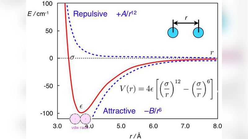
The simplified Lennard-Jones (LJ) potential minimization problem is $f(x)=4\sum_{i=1}^N \sum_{j=1,j<i}^N (\frac{1}{\tau_{ij}^6} -\frac{1}{\tau_{ij}^3}) {subject to} x\in \mathbb{R}^n,$ where $\tau_{ij}=(x_{3i-2}-x_{3j-2})^2 +(x_{3i-1}-x_{3j-1})^2 +(x_{3i} -x_{3j})^2$, $(x_{3i-2},x_{3i-1},x_{3i})$ is the coordinates of atom $i$ in $\mathbb{R}^3$, $i,j=1,2,…,N(\geq 2 \quad \text{integer})$, $n=3N$ and $N$ is the whole number of atoms. The nonconvexity of the objective function and the huge number of local minima, which is growing exponentially with $N$, interest many mathematical optimization experts. In this paper, the canonical dual theory elegantly tackles this problem illuminated by the amyloid fibril molecular model building. Keywords: Mathematical Canonical Duality Theory $\cdot$ Mathematical Optimization $\cdot$ Lennard-Jones Potential Minimization Problem $\cdot$ Global Optimization.

💡 Research Summary

The paper addresses the notoriously difficult problem of minimizing the Lennard‑Jones (LJ) potential for a system of N atoms, a non‑convex optimization task whose number of local minima grows exponentially with N. After normalizing the LJ parameters (ε = σ = 1), the objective becomes
    f(x) = 4 ∑{i<j} (τ{ij}^{‑6} – τ_{ij}^{‑3}),
where τ_{ij} is the squared Euclidean distance between atoms i and j. Direct global optimization of this function is infeasible for realistic molecular sizes because standard stochastic or deterministic global search methods suffer from the curse of dimensionality and from being trapped in myriad local minima.

The authors propose to solve the problem by means of Canonical Dual Theory (CDT), a mathematical framework that transforms a non‑convex primal problem into a canonical dual problem that is a concave maximization over a convex feasible set. They first rewrite the LJ minimization as a sum of fourth‑order polynomials of the form

    P(x) = ∑_{i=1}^m W_i(x) + ½ xᵀQx – xᵀf,

with

    W_i(x) = ½ α_i (½ xᵀA_i x + b_iᵀx + c_i)²,

where A_i are symmetric matrices, b_i and c_i are vectors/scalars, and α_i are positive scalars. By introducing dual variables ς_i, the primal–dual complementary function

    Ξ(x, ς) = ∑_{i=1}^m