A recursive divide-and-conquer approach for sparse principal component analysis
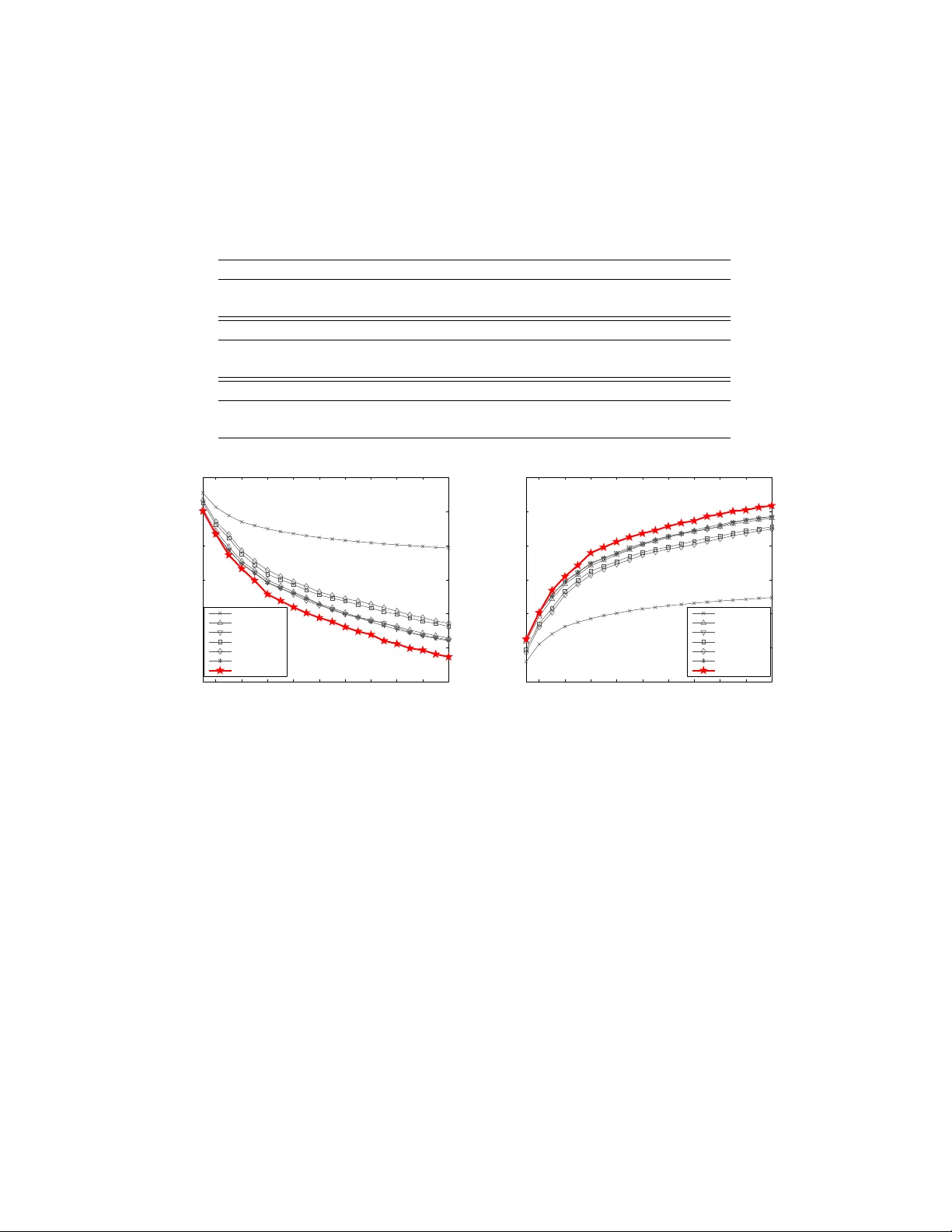
In this paper, a new method is proposed for sparse PCA based on the recursive divide-and-conquer methodology. The main idea is to separate the original sparse PCA problem into a series of much simpler sub-problems, each having a closed-form solution.…
Authors: Qian Zhao, Deyu Meng, Zongben Xu
A recursiv e divide-and-conquer approac h for sparse principal comp onen t analysis Qian Zhao , Deyu Meng ∗ , Zongb en Xu Institute for Information and System Scienc es, Scho ol of Mathematics and Statistics, Xi’an Jiaotong University, Xi’an 710049, PR China Abstract In this pap er, a new metho d is prop osed for sparse PCA based on the re- cursiv e divide-and-conquer methodology . The main idea is to separate the original sparse PCA problem in to a series of muc h simpler sub-problems, eac h ha ving a closed-form solution. By recursively solving these sub-problems in an analytical wa y , an efficient algorithm is constructed to solve the sparse PCA problem. The algorithm only in volv es simple computations and is th us easy to implemen t. The prop osed metho d can also b e very easily ex- tended to other sparse PCA problems with certain constraints, suc h as the nonnegativ e sparse PCA problem. F urtherm ore, w e ha ve sho wn that the prop osed algorithm con verges to a stationary p oint of the problem, and its computational complexity is approximately linear in b oth data size and di- mensionalit y . The effectiveness of the prop osed metho d is substan tiated by extensiv e exp eriments implemen ted on a series of synthetic and real data in b oth reconstruction-error-minimization and data-v ariance-maximization viewp oin ts. Keywor ds: F ace recognition, nonnegativity , principal comp onen t analysis, recursiv e divide-and-conquer, sparsity . ∗ Corresp onding author. T el.: +86 13032904180; fax: +86 2982668559. Email addr esses: zhao.qian@stu.xjtu.edu.cn (Qian Zhao), dymeng@mail.xjtu.edu.cn (Deyu Meng), zbxu@mail.xjtu.edu.cn (Zongben Xu) Pr eprint submitte d to Elsevier June 1, 2021 1. In tro duction Principal comp onen t analysis (PCA) is one of the most classical and p opular to ols for data analysis and dimensionality reduction, and has a wide range of successful applications throughout science and engineering [1]. By seeking the so-called principal comp onents (PCs), along whic h the data v ari- ance is maximally preserved, PCA can alw ays capture the in trinsic laten t structure underlying data. Suc h information greatly facilitates man y further data pro cessing tasks, such as feature extraction and pattern recognition. Despite its many adv an tages, the con ven tional PCA suffers from the fact that each comp onen t is generally a linear combination of all data v ariables, and all weigh ts in the linear combination, also called loadings, are t ypically non-zeros. In man y applications, ho wev er, the original v ariables ha v e mean- ingful physical interpretations. In biology , for example, each v ariable of gene expression data corresponds to a certain gene. In these cases, the derived PC loadings are alwa ys exp ected to b e sparse (i.e. con tain fewer non-zeros) so as to facilitate their interpretabilit y . Moreo ver, in certain applications, such as financial asset trading, the sparsit y of the PC loadings is esp ecially exp ected since few er nonzero loadings imply fewer transaction costs. Accordingly , sparse PCA has attracted muc h atten tion in the recent decade, and a v ariet y of metho ds for this topic hav e b een developed [2 – 23]. The first attempt for this topic is to make certain p ost-processing transfor- mation, e.g. rotation [2] b y Jolliffe and simple thresholding [3] by Cadima and Jolliffe, on the PC loadings obtained by the conv entional PCA to en- force sparsity . Jolliffe and Uddin further adv anced a SCoTLASS algorithm b y sim ultaneously calculating sparse PCs on the PCA mo del with additional l 1 -norm p enalt y on loading v ectors [4]. Better results ha v e b een ac hiev ed b y the SPCA algorithm of Zou et al., which was developed based on it- erativ e elastic net regression [5]. D’Aspremon t et al. prop osed a method, called DSPCA, for finding sparse PCs by solving a sequence of semidefi- nite programming (SDP) relaxations of sparse PCA [6]. Shen and Huang dev elop ed a series of metho ds called sPCA-rSVD (including sPCA-rSVD l 0 , sPCA-rSVD l 1 , sPCA-rSVD S C AD ), computing sparse PCs b y low-rank ma- trix factorization under multiple sparsity-including p enalties [7]. Journ´ ee et al. designed four algorithms, denoted as GP ow er l 0 , GP ow er l 1 , GP ow er l 0 ,m , and GPo wer l 1 ,m , resp ectiv ely , for sparse PCA by form ulating the issue as non-conca ve maximization problems with l 0 - or l 1 -norm sparsity-inducing p enalties and extracting single unit sparse PC sequentially or blo c k units 2 ones sim ultaneously [8]. Based on probabilistic generativ e mo del of PCA, some metho ds hav e also b een attained [9 – 12], e.g. the EMPCA method deriv ed b y Sigg and Buhmann for sparse and/or nonnegative sparse PCA [9]. Srip erum budur et al. pro vided an iterativ e algorithm called DCPCA, where eac h iteration consists of solving a quadratic programming (QP) prob- lem [13, 14]. Recen tly , Lu and Zhang developed an augmented Lagrangian metho d (ALSPCA briefly) for sparse PCA by solving a class of non-smo oth constrained optimization problems [15]. Additionally , d’Aspremont deriv ed a PathSPCA algorithm that computes a full set of solutions for all target n umbers of nonzero co efficien ts [16]. There are mainly tw o metho dologies utilized by the current research on sparse PCA problem. The first is the greedy approac h, including DSPCA [6], sPCA-rSVD [7], EMPCA [9], P athSPCA [16], etc. These metho ds mainly fo cus on the solving of one-sparse-PC mo del, and more sparse PCs can b e sequen tially calculated on the deflated data matrix or data cov ariance [24]. Under this metho dology , the first several sparse PCs underlying the data can generally b e prop erly extracted, while the computation for more sparse PCs tends to b e incremen tally inv alidated due to the cum ulation of compu- tational error. The second is the blo c k approac h. Typical metho ds include SCoTLASS [4], GP ow er l 0 ,m , GP ow er l 1 ,m [8], ALSPCA [15], etc. These meth- o ds aim to calculate multiple sparse PCs at once by utilizing certain blo c k optimization tec hniques. The blo c k approach for sparse PCA is exp ected to b e more efficien t than the greedy one to sim ultaneously attain multiple PCs, while is generally difficult to elaborately rectify each individual sparse PC based on some sp ecific requirements in practice (e.g. the num b er of nonzero elemen ts in each PC). In this paper, a new metho dology , called the recursive divide-and-conquer (ReDaC briefly), is emplo yed for solving the sparse PCA problem. The main idea is to decomp ose the original large and complex problem of sparse PCA in to a series of small and simple sub-problems, and then recursively solve them. Each of these sub-problems has a closed-form solution, which makes the new metho d simple and v ery easy to implemen t. On one hand, as com- pared with the greedy approac h, the new metho d is exp ected to in tegratively ac hieve a collection of appropriate sparse PCs of the problem by iteratively rectifying each sparse PC in a recursiv e w ay . The group of sparse PCs at- tained by the prop osed metho d is further prov ed b eing a stationary solution of the original sparse PCA problem. On the other hand, as compared with the blo c k approach, the new method can easily handle the constraints su- 3 p erimposed on eac h individual sparse PC, suc h as certain sparsit y and/or nonnegativ e constraints. Besides, the computational complexity of the pro- p osed metho d is approximately linear in b oth data size and dimensionalit y , whic h makes it well-suited to handle large-scale problems of sparse PCA. In what follo ws, the main idea and the implementation details of the prop osed metho d are first in tro duced in Section 2. Its conv ergence and com- putational complexity are also analyzed in this section. The effectiv eness of the prop osed metho d is comprehensively substantiated based on a series of empirical studies in Section 3. Then the pap er is concluded with a summary and outlo ok for future research. Throughout the pap er, w e denote matrices, v ectors and scalars b y the upp er-case bold-faced letters, low er-case b old-faced letters, and lo wer-case letters, resp ectiv ely . 2. The recursiv e divide-and-conquer metho d for sparse PCA In the following, w e first introduce the fundamen tal mo dels for the sparse PCA problem. 2.1. Basic mo dels of sp arse PCA Denote the input data matrix as X = [ x 1 , x 2 , . . . , x n ] T ∈ R n × d , where n and d are the size and the dimensionality of the given data, resp ectively . After a lo cation transformation, w e can assume all { x i } n i =1 to ha ve zero mean. Let Σ = 1 n X T X ∈ R d × d b e the data cov ariance matrix. The classical PCA can b e solved through t wo types of optimization models [1]. The first is constructed b y finding the r ( ≤ d )-dimensional linear subspace where the v ariance of the input data X is maximized [25]. On this data- v ariance-maximization viewp oin t, the PCA is formulated as the follo wing optimization mo del: max V T r( V T ΣV ) s.t. V T V = I , (1) where T r( A ) denotes the trace of the matrix A and V = ( v 1 , v 2 , . . . , v r ) ∈ R d × r denotes the array of PC loading v ectors. The second is form ulated by seeking the r -dimensional linear subspace on which the pro jected data and the original ones are as close as p ossible [26]. On this reconstruction-error- minimization viewp oin t, the PCA corresp onds to the following mo del: min U , V X − UV T 2 F s.t. V T V = I , (2) 4 where k A k F is the F rob enius norm of A , V ∈ R d × r is the matrix of PC loading arra y and U = ( u 1 , u 2 , . . . , u r ) ∈ R n × r is the matrix of pro jected data. The tw o mo dels are intrinsically equiv alen t and can attain the same PC loading v ectors [1]. Corresp onding to the PCA mo dels (1) and (2), the sparse PCA problem has the follo wing tw o mathematical formulations 1 : max V T r( V T ΣV ) s.t. v T i v i = 1 , k v i k p ≤ t i ( i = 1 , 2 , . . . , r ) , (3) and min U , V X − UV T 2 F s.t. v T i v i = 1 , k v i k p ≤ t i ( i = 1 , 2 , . . . , r ) , (4) where p = 0 or 1 and the corresp onding k v k p denotes the l 0 - or the l 1 - norm of v , resp ectiv ely . Note that the inv olved l 0 or l 1 p enalt y in the ab ov e mo dels (3) and (4) tends to enforce sparsit y of the output PCs. Metho ds constructed on (3) include SCoTLASS [4], DSPCA [6], DCPCA [13, 14], ALSPCA [15], etc., and those related to (4) include SPCA [5], sPCA-rSVD [7], SPC [19], GPo w er [8], etc. In this pap er, we will construct our metho d on the reconstruction-error-minimization mo del (4), while our exp erimen ts will verify that the prop osed metho d also p erforms well based on the data- v ariance-maximization criterion. 2.2. De c omp ose original pr oblem into smal l and simple sub-pr oblems The ob jectiv e function of the sparse PCA mo del (4) can b e equiv alently form ulated as follows: X − UV T 2 F = X − X r j =1 u j v T j 2 F = E i − u i v T i 2 F , where E i = X − P j 6 = i u j v T j . It is then easy to separate the original large minimization problem, which is with resp ect to U and V , into a series of small minimization problems, which are eac h with resp ect to a column v ector u i of U and v i of V for i = 1 , 2 , . . . , r , resp ectively , as follo ws: min v i E i − u i v T i 2 F s.t. v T i v i = 1 , k v i k p ≤ t i , (5) 1 It should b e noted that the orthogonality constraints of PC loadings in (1) and (2) are not imp osed in (3) and (4). This is b ecause simultaneously enforcing sparsity and orthogonalit y is generally a very difficult (and p erhaps unnecessary) task. Like most of the existing sparse PCA metho ds [5–8], w e do not enforce orthogonal PCs in the mo dels. 5 and min u i E i − u i v T i 2 F . (6) Through recursively optimizing these small sub-problems, the recursiv e divide- and-conquer (ReDaC) method for solving the sparse PCA mo del (4) can then b e naturally constructed. It is v ery fortunate that b oth the minimization problems in (5) and (6) ha ve closed-form solutions. This implies that the to-b e-constructed ReDaC metho d can b e fast and efficient, as presented in the following sub-sections. 2.3. The close d-form solutions of (5) and (6) F or the con venience of denotation, we first rewrite (5) and (6) as the follo wing forms: min v E − uv T 2 F s.t. v T v = 1 , k v k p ≤ t, (7) and min u E − uv T 2 F , (8) where u is n -dimensional and v is d -dimensional. Since the ob jectiv e function E − uv T 2 F can b e equiv alen tly transformed as: E − uv T 2 F = T r(( E − uv T ) T ( E − uv T )) = k E k 2 F − 2T r( E T uv T ) + T r( vu T uv T ) = k E k 2 F − 2 u T Ev + u T uv T v , (7) and (8) are equiv alen t to the following optimization problems, resp ec- tiv ely: max v ( E T u ) T v s.t. v T v = 1 , k v k p ≤ t, (9) and min u u T u − 2( Ev ) T u . (10) The closed-form solutions of (9) and (10), i.e. (7) and (8), can then b e presen ted as follows. W e present the closed-form solution to (8) in the following theorem. Theorem 1. The optimal solution of (8) is u ∗ ( v ) = Ev . 6 The theorem is very easy to prov e b y calculating where the gradient of u T u − 2( Ev ) T u is equal to zero. W e th us omit the pro of. In the p = 0 case, the closed-form solution to (9) is presen ted in the follow- ing theorem. Here, w e denote w = E T u , and hard λ ( w ) the hard thresholding function, whose i -th element corresp onds to I ( | w i | ≥ λ ) w i , where w i is the i -th elemen t of w and I ( x ) (equals 1 if x is ture, and 0 otherwise) is the indicator function. The pro of of the theorem is provided in App endix A. Theorem 2. The optimal solution of max v w T v s.t. v T v = 1 , k v k 0 ≤ t, (11) is given by: v ∗ 0 ( w , t ) = φ, t < 1 , hard θ k ( w ) k hard θ k ( w ) k 2 , k ≤ t < k + 1 ( k = 1 , 2 , . . . , d − 1) , w k w k 2 t ≥ d , wher e θ k denotes the k -th lar gest element of | w | . In the ab o v e theorem, φ denotes the empty set, implying that when t < 1, the optim um of (11) do es not exist. In the p = 1 case, (7) has the following closed-form solution. In the theorem, we denote f w ( λ ) = sof t λ ( w ) k sof t λ ( w ) k 2 , where sof t λ ( w ) represen ts the soft thresholding function sig n ( w )( | w | − λ ) + , where ( x ) + represen ts the v ec- tor attained by pro jecting x to its nonnegative orthan t, and ( I 1 , I 2 , . . . , I d ) denotes the p erm utation of (1 , 2 , . . . , d ) based on the ascending order of | w | = ( | w 1 | , | w 2 | , . . . , | w d | ) T . Theorem 3. The optimal solution of max v w T v s.t. v T v = 1 , k v k 1 ≤ t, (12) is given by: v ∗ 1 ( w , t ) = φ, t < 1 , f w ( λ k ) , k f w ( | w I k | ) k 1 ≤ t < k f w ( | w I k − 1 | ) k 1 ( k = 2 , 3 , . . . , d − 1) , f w ( λ 1 ) , k f w ( | w I 1 | ) k 1 ≤ t < √ d, f w (0) , t ≥ √ d, 7 wher e for k = 1 , 2 , . . . , d − 1 , λ k = ( m − t 2 )( P m i =1 a i ) − p t 2 ( m − t 2 )( m P m i =1 a 2 i − ( P m i =1 a i ) 2 ) m ( m − t 2 ) , wher e ( a 1 , a 2 , . . . , a m ) = ( | w I k | , | w I k +1 | , . . . , | w I d | ) , m = d − k + 1 . It should be noted that we hav e prov ed that k f w ( | w I d − 1 | ) k 1 = 1 and k f w ( λ ) k 1 is a monotonically decreasing function with resp ect to λ in Lemma 1 of the app endix. This means that we can conduct the optim um v ∗ ( w ) of the optimization problem (7) for an y w based on the ab o v e theorem. The ReDaC algorithm can then b e easily constructed based on Theorems 1-3. 2.4. The r e cursive divide-and-c onquer algorithm for sp arse PCA The main idea of the new algorithm is to recursively optimize each col- umn, u i of U or v i of V for i = 1 , 2 , . . . , r , with other u j s and v j s ( j 6 = i ) fixed. The pro cess is summarized as follows: • Up date eac h column v i of V for i = 1 , 2 , . . . , r by the closed-form solution of (5) attained from Theorem 2 (for p = 0) or Theorem 3 (for p = 1). • Up date each column u i of U for i = 1 , 2 , . . . , r by the closed-form solution of (6) calculated from Theorem 1. Through implemen ting the abov e pro cedures iteratively , U and V can b e recursiv ely up dated un til the stopping criterion is satisfied. W e summarize the aforemen tioned ReDaC technique as Algorithm 1. W e then briefly discuss ho w to sp ecify the stopping criterion of the algo- rithm. The ob jective function of the sparse PCA mo del (4) is monotonically decreasing in the iterative pro cess of Algorithm 1 since eac h of the step 5 and step 6 in the iterations mak es an exact optimization for a column v ector u i of U or v i of V , with all of the others fixed. W e can thus terminate the iterations of the algorithm when the up dating rate of U or V is smaller than some preset threshold, or the maxim um num b er of iterations is reached. No w we briefly analyze the computational complexity of the prop osed ReDaC algorithm. It is evident that the computational complexity of Algo- rithm 1 is essen tially determined by the iterations b et ween step 5 and step 8 Algorithm 1 ReDaC algorithm for sparse PCA Input: Data matrix X ∈ R n × d , n um b er of sparse PCs r , sparsit y parameters t = ( t 1 , . . . , t r ). 1: Initialize U = ( u 1 , u 2 , . . . , u r ) ∈ R n × r , V = ( v 1 , u 2 , . . . , v r ) ∈ R d × r . 2: rep eat 3: for i = 1 , . . . r do 4: Compute E i = X − P j 6 = i u j v T j . 5: Up date v i via solving (5) based on Theorem 2 (for p = 0) or Theorem 3 (for p = 1). 6: Up date u i via solving (6) based on Theorem 1. 7: end for 8: un til stopping criterion satisfied. Output: The sparse PC loading v ectors V = ( v 1 , v 2 , . . . , v r ). 6, i.e. the calculation of the closed-form solutions of v i and u i of V and U , resp ectiv ely . T o compute u i , only simple op erations are inv olv ed and the computation needs O ( nd ) cost. T o compute v i , a sorting for the elements of the d -dimensional v ector | w | = | E T u | is required, and the total compu- tational cost is around O ( nd log d ) by applying the w ell-known heap sorting algorithm [27]. The whole pro cess of the algorithm thus requires around O ( rnd log d ) computational cost in eac h iteration. That is, the computa- tional complexit y of the prop osed algorithm is approximately linear in b oth the size and the dimensionalit y of input data. 2.5. Conver genc e analysis In this section w e ev aluate the conv ergence of the prop osed algorithm. The con vergence of our algorithm can actually b e implied by the mono- tonic decrease of the cost function of (4) during the iterations of the al- gorithm. In sp ecific, in each iteration of the algorithm, step 5 and step 6 optimize the column vector u i of U or v i of V , with all of the others fixed, resp ectiv ely . Since the ob jective function of (4) is evidently lo wer b ounded ( ≥ 0), the algorithm is guaranteed to b e conv ergent. W e wan t to go a further step to ev aluate where the algorithm conv erges. Based on the form ulation of the optimization problem (4), w e can construct 9 a sp ecific function as follows: f ( u 1 , . . . , u r , v 1 , . . . , v r ) = f 0 ( u 1 , . . . , u r , v 1 , . . . , v r ) + r X i =1 f i ( v i ) . (13) where f 0 ( u 1 , . . . , u r , v 1 , . . . , v r ) = X − UV T 2 F = X − X r i =1 u i v T i 2 F , and for eac h of i = 1 , . . . , r , f i ( v i ) is an indicator function defined as: f i ( v i ) = ( 0 , if k v i k p ≤ t i and v T i v i = 1 , ∞ , otherwise . It is then easy to show that the constrained optimization problem (4) is equiv alen t to the unconstrained problem min { u i , v i } r i =1 f ( u 1 , . . . , u r , v 1 , . . . , v r ) . (14) The prop osed ReDaC algorithm can then b e view ed as a blo c k co ordinate descen t (BCD) metho d for solving (14) [28], by alterativ ely optimizing u i , v i , i = 1 , 2 , . . . , r , resp ectiv ely . Then the follo wing theorem implies that our algorithm can con verge to a stationary p oin t of the problem. Theorem 4 ([28]) . Assume that the level set X 0 = { x : f ( x ) ≤ f ( x 0 ) } is c omp act and that f is c ontinuous on X 0 . If f ( u 1 , . . . , u r , v 1 , . . . , v r ) is r e gular and has at most one minimum in e ach u i and v i with others fixe d for i = 1 , 2 , . . . , r , then the se quenc e ( u 1 , . . . , u r , v 1 , . . . , v r ) gener ate d by A lgorithm 1 c onver ges to a stationary p oint of f . In the ab o v e theorem, the assumption that the function f , as defined in (14), is regular holds under the condition that dom ( f 0 ) is op en and f 0 is Gateaux-differen tiable on dom ( f 0 ) (Lemma 3.1 under Condition A1 in [28]). Based on Theorems 1-3, we can also easily see that f ( u 1 , . . . , u r , v 1 , . . . , v r ) has unique minim um in eac h u i and v i with others fixed. The ab o ve theorem can then b e naturally follow ed b y Theorem 4.1(c) in [28]. Another adv antage of the prop osed ReDaC metho dology is that it can b e easily extended to other sparse PCA applications when certain constraints are needed for output sparse PCs. In the follo wing section we giv e one of the extensions of our metho dology — nonnegative sparse PCA problem. 10 2.6. The R eDaC metho d for nonne gative sp arse PCA The nonnegative sparse PCA [29] problem differs from the conv entional sparse PCA in its nonnegativity constrain t imp osed on the output sparse PCs. The nonnegativity prop ert y of this problem is esp ecially imp ortan t in some applications suc h as micro economics, en vironmental science, biology , etc. [30]. The corresp onding optimization mo del is written as follows: min U , V X − UV T 2 F s.t. v T i v i = 1 , k v i k p ≤ t i , v i 0 ( i = 1 , 2 , . . . , r ) , (15) where v i 0 means that each element of v i is greater than or equal to 0. By utilizing the similar recursiv e divide-and-conquer strategy , this prob- lem can b e separated into a series of small minimization problems, eac h with resp ect to a column v ector u i of U and v i of V for i = 1 , 2 , . . . , r , resp ectiv ely , as follo ws: min v i E i − u i v T i 2 F s.t. v T i v i = 1 , k v i k p ≤ t i , v i 0 (16) and min u i E i − u i v T i 2 F , (17) where p = 0 or 1. Since (17) is of the same formulation as (6), w e only need to discuss ho w to solv e (16). F or the con venience of denotation, w e first rewrite (16) as: min v E − uv T 2 F s.t. v T v = 1 , k v k p ≤ t, v 0 . (18) The closed-form solution of (18) is giv en in the following theorem. Theorem 5. The close d-form solution of (18) is v ∗ p (( w ) + , t ) ( p = 0 , 1 ), wher e w = E T u , and v ∗ 0 ( · , · ) and v ∗ 1 ( · , · ) ar e define d in The or em 2 and The- or em 3, r esp e ctively. By virtue of the closed-form solution of (18) giv en b y Theorem 5, w e can no w construct the ReDaC algorithm for solving nonnegative sparse PCA mo del (15). Since the algorithm differs from Algorithm 1 only in step 5 (i.e. up dating of v i ), w e only list this step in Algorithm 2. W e then substan tiate the effectiv eness of the proposed ReDaC algorithms for sparse PCA and nonnegativ e sparse PCA through exp erimen ts in the next section. 11 Algorithm 2 ReDaC algorithm for nonnegative sparse PCA 5: Up date v i via solving (16) based on Theorem 5. 3. Exp erimen ts T o ev aluate the p erformance of the prop osed ReDaC algorithm on the sparse PCA problem, w e conduct exp erimen ts on a series of synthetic and real data sets. All the exp erimen ts are implemen ted on Matlab 7.11(R2010b) platform in a PC with AMD Athlon(TM) 64 X2 Dual 5000+@2.60 GHz (CPU), 2GB (memory), and Windo ws XP (OS). In all exp erimen ts, the SVD metho d is utilized for initialization. The prop osed algorithm under b oth p = 0 and p = 1 w as implemented in all exp erimen ts and mostly hav e a similar p erformance. W e th us only list the b etter one throughout. 3.1. Synthetic simulations Tw o synthetic data sets are first utilized to ev aluate the p erformance of the prop osed algorithm on reco vering the ground-truth sparse principal comp onen ts underlying data. 3.1.1. Hastie data Hastie data set w as first prop osed b y Zou et al. [5] to illustrate the adv an tage of sparse PCA ov er conv entional PCA on sparse PC extraction. So far this data set has b ecome one of the most frequently utilized benchmark data for testing the effectiv eness of sparse PCA methods. The data set is generated in the following w a y: first, three hidden factors V 1 , V 2 and V 3 are created as: V 1 ∼ N (0 , 290) , V 2 ∼ N (0 , 300) , V 3 = 0 . 3 V 1 + 0 . 925 V 2 + ε, where ε ∼ N (0 , 1), and V 1 , V 2 and ε are indep endent; afterw ards, 10 observ- able v ariables are generated as: X i = V 1 + ε 1 i , i = 1 , 2 , 3 , 4 , X i = V 2 + ε 2 i , i = 5 , 6 , 7 , 8 , X i = V 3 + ε 3 i , i = 9 , 10 , where ε j i ∼ N (0 , 1) and all ε j i s are indep enden t. The data so generated are of intrinsic sparse PCs [5]: the first recov ers the factor V 2 only using ( X 5 , X 6 , X 7 , X 8 ), and the second reco vers V 1 only utilizing ( X 1 , X 2 , X 3 , X 4 ). 12 W e generate 100 sets of data, eac h contains 1000 data generated in the aforemen tioned w ay , and apply Algorithm 1 to them to extract the first t wo sparse PCs. The results sho w that our algorithm can p erform w ell in all exp erimen ts. In sp ecific, the prop osed ReDaC algorithm faithfully deliv ers the ground-truth sparse PCs in all exp erimen ts. The effectiveness of the prop osed algorithm is thus easily substantiated in this series of b enc hmark data. 3.1.2. Synthetic toy data As [7] and [8], w e adopt another interesting to y data, with in trinsic sparse PCs, to ev aluate the p erformance of the proposed method. The data are gen- erated from the Gaussian distribution N ( 0 , Σ ) with mean 0 and cov ariance Σ ∈ R 10 × 10 , whic h is calculated by Σ = 10 X j =1 c j v j v T j . Here, ( c 1 , c 2 , ..., c 10 ), the eigenv alues of the cov ariance matrix Σ , are pre- sp ecified as (250 , 240 , 50 , 50 , 6 , 5 , 4 , 3 , 2 , 1), resp ectiv ely , and ( v 1 , v 2 , ..., v 10 ) are 10-dimensional orthogonal v ectors, formulated by v 1 = (0 . 422 , 0 . 422 , 0 . 422 , 0 . 422 , 0 , 0 , 0 , 0 , 0 . 380 , 0 . 380) T , v 2 = (0 , 0 , 0 , 0 , 0 . 489 , 0 . 489 , 0 . 489 , 0 . 489 , − 0 . 147 , 0 . 147) T , and the rest b eing generated by applying Gram-Schmidt orthonormalization to 8 randomly v alued 10-dimensional vectors. It is easy to see that the data generated under this distribution are of first tw o sparse PC vectors v 1 and v 2 . F our series of exp erimen ts, each in volving 1000 sets of data generated from N ( 0 , Σ ), are utilized, with sample sizes 500, 1000, 2000, 5000, re- sp ectiv ely . F or eac h exp erimen t, the first tw o PCs, ˆ v 1 and ˆ v 2 , are cal- culated by a sparse PCA metho d and then if b oth | ˆ v T 1 v 1 | ≥ 0 . 99 and | ˆ v T 2 v 2 | ≥ 0 . 99 are satisfied, the metho d is considered as a success. The prop osed ReDaC metho d, together with the con ven tional PCA and 12 cur- ren t sparse PCA metho ds, including SPCA [5], DSPCA [6], PathSPCA [16], sPCA-rSVD l 0 , sPCA-rSVD l 1 , sPCA-rSVD S C AD [7], EMPCA [9], GPo wer l 0 , GP ow er l 1 , GPo wer l 0 ,m , GPo wer l 1 ,m [8] and ALSPCA [15], ha ve b een im- plemen ted, and the success times for four series of exp erimen ts hav e b een recorded and summarized, resp ectiv ely . The results are listed in T able 1. 13 T able 1: Comparison of success times of PCA and differen t sparse PCA metho ds in syn- thetic to y exp erimen ts with sample size v arying. The b est results are highlighted in b old. n = 500 n = 1000 n = 2000 n = 5000 PCA 0 0 0 0 SPCA 566 673 756 839 DSPCA 211 203 138 62 P athSPCA 189 187 186 171 sPCA-rSVD l 0 646 702 797 906 sPCA-rSVD l 1 649 715 806 909 sPCA-rSVD SCAD 649 715 806 909 EMPCA 649 715 806 909 GP ow er l 0 155 154 155 139 GP ow er l 1 122 127 126 126 GP ow er l 0 ,m 91 76 71 16 GP ow er l 1 ,m 90 92 88 82 ALSPCA 669 749 826 927 ReDaC 676 748 827 928 The adv antage of the prop osed ReDaC algorithm can b e easily observ ed from T able 1. In sp ecific, our metho d alwa ys attains the highest or second highest success times (in the size 1000 case, 1 less than ALSPCA) as com- pared with the other utilized metho ds in all of the four series of exp eriments. Considering that the ALSPCA metho d, which is the only comparable method in these exp erimen ts, utilizes strict constraints on the orthogonalit y of out- put PCs while the ReDaC metho d do es not utilize any prior ground-truth information of data, the capabilit y of the prop osed metho d on sparse PCA calculation can b e more prominently verified. 3.2. Exp eriments on r e al data In this section, we further ev aluate the p erformance of the prop osed ReDaC metho d on tw o real data sets, including the pitprops and colon data. Two quantitativ e criteria are employ ed for p erformance assessmen t. They are designed in the viewpoints of reconstruction-error-minimization and data-v ariance-maximization, resp ectiv ely , just corresp onding to the original form ulations (4) and (3) for sparse PCA problem. • R e c onstruction-err or-minimization criterion: RRE. Once sparse PC loading matrix V is obtained by a metho d, the input data can then b e reconstructed by ˆ X = ˆ UV T , where ˆ U = XV ( V T V ) − 1 , attained b y 14 the least square metho d. Then the relativ e reconstruction error (RRE) can b e calculated by RRE = k X − ˆ X k F k X k F , to assess the p erformance of the utilized method in data reconstruction p oin t of view. • Data-varianc e-maximization criterion: PEV. After attaining the sparse PC loading matrix V , the input data can then b e reconstructed by ˆ X = XV ( V T V ) − 1 V T , as aforemen tioned. And th us the v ariance of the reconstructed data can be computed b y T r( 1 n ˆ X T ˆ X ). The p ercentage of explained v ariance (PEV, [7]) of the reconstructed data from the original one can then b e calculated by PEV = T r( 1 n ˆ X T ˆ X ) T r( 1 n X T X ) × 100% = T r( ˆ X T ˆ X ) T r( X T X ) × 100% , to ev aluate the p erformance of the utilized metho d in data v ariance p oin t of view. 3.2.1. Pitpr ops data The pitprops data set, consisting of 180 observ ations and 13 measured v ariables, was first introduced by Jeffers [31] to sho w the difficulty of inter- preting PCs. This data set is one of the most commonly utilized examples for sparse PCA ev aluation, and th us is also emplo y ed to testify the effec- tiv eness of the prop osed ReDaC metho d. The comparison metho ds include SPCA [5], DSPCA [6], PathSPCA [16], sPCA-rSVD l 0 , sPCA-rSVD l 1 , sPCA- rSVD S C AD [7], EMPCA [9], GPo w er l 0 , GPo wer l 1 , GPo wer l 0 ,m , GPo wer l 1 ,m [8] and ALSPCA [15]. F or eac h utilized metho d, 6 sparse PCs are extracted from the pitprops data, with different cardinalit y settings: 8-5-6-2-3-2 (al- together 26 nonzero elements), 7-4-4-1-1-1 (altogether 18 nonzero elements, as set in [5]) and 7-2-3-1-1-1 (altogether 15 nonzero elements, as set in [6]), resp ectiv ely . In eac h exp erimen t, b oth the RRE and PEV v alues, as defined ab o v e, are calculated, and the results are summarized in T able 2. Figure 1 further shows the the RRE and PEV curves attained b y different sparse PCA metho ds in all exp erimen ts for more illumination. It should b e noted that the GPo wer l 0 ,m , GP ow er l 1 ,m and ALSPCA metho ds emplo y the block metho dology , as introduced in the introduction of the pap er, and calculate 15 T able 2: Performance comparison of different sparse PCA metho ds on pitprops data with differen t cardinalit y settings. The best result in each exp erimen t is highlighted in b old. 8-5-6-2-3-2(26) 7-4-4-1-1-1(18) 7-2-3-1-1-1(15) RRE PEV RRE PEV RRE PEV SPCA 0.4162 82.68% 0.4448 80.22% 0.4459 80.11% DSPCA 0.4303 81.48% 0.4563 79.18% 0.4771 77.23% P athSPCA 0.4080 83.35% 0.4660 80.11% 0.4457 80.13% sPCA-rSVD l 0 0.4139 82.87% 0.4376 80.85% 0.4701 77.90% sPCA-rSVD l 1 0.4314 81.39% 0.4427 80.40% 0.4664 78.25% sPCA-rSVD SCAD 0.4306 81.45% 0.4453 80.17% 0.4762 77.32% EMPCA 0.4070 83.44% 0.4376 80.85% 0.4451 80.18% GP ow er l 0 0.4092 83.26% 0.4400 80.64% 0.4457 80.13% GP ow er l 1 0.4080 83.35% 0.4460 80.11% 0.4457 80.13% GP ow er l 0 ,m 0.4224 82.16% 0.5089 74.10% 0.4644 78.44% GP ow er l 1 ,m 0.4187 82.46% 0.4711 77.81% 0.4589 78.94% ALSPCA 0.4168 82.63% 0.4396 80.67% 0.4537 79.42% ReDaC 0.4005 83.50% 0.4343 81.14% 0.4420 80.46% all sparse PCs at once while cannot sequentially deriv e different n um b ers of sparse PCs with preset cardinalit y settings. Th us the results of these meth- o ds rep orted in T able 2 are calculated with the total sparse PC cardinalities b eing 26, 18 and 15, resp ectively , and are not included in Figure 1. It can b e seen from T able 2 that under all cardinalit y settings of the first 6 PCs, the prop osed ReDaC method alw a ys ac hieves the low est RRE and highest PEV v alues among all the comp eting metho ds. This means that the ReDaC method is adv antageous in b oth reconstruction-error-minimization and data-v ariance-maximization viewp oin ts. F urthermore, from Figure 1, it is easy to see the sup eriorit y of the ReDaC metho d. In sp ecific, for different n umber of extracted sparse PC comp onents, the prop osed ReDaC metho d can alw a ys get the smallest RRE v alues and the largest PEV v alues, as compared with the other utilized sparse PCA metho ds, in the exp eriments. This further substan tiates the effectiveness of the prop osed ReDaC metho d in b oth reconstruction-error-minimization and data-v ariance-maximization views. 3.2.2. Colon data The colon data set [32] consists of 62 tissue samples with the gene ex- pression profiles of 2000 genes extracted from DNA micro-array data. This is a t ypical data set with high-dimension and lo w-sample-size prop ert y , and 16 1 2 3 4 5 6 0.4 0.5 0.6 0.7 0.8 0.9 Number of Sparse Principal Components RRE Cardinality Setting: 8−5−6−2−3−2 1 2 3 4 5 6 20% 30% 40% 50% 60% 70% 80% 90% Number of Sparse Principal Components PEV 1 2 3 4 5 6 0.4 0.5 0.6 0.7 0.8 0.9 Number of Sparse Principal Components RRE Cardinality Setting: 7−4−4−1−1−1 1 2 3 4 5 6 20% 30% 40% 50% 60% 70% 80% 90% Number of Sparse Principal Components PEV 1 2 3 4 5 6 0.4 0.5 0.6 0.7 0.8 0.9 Number of Sparse Principal Components RRE Cardinality Setting: 7−2−3−1−1−1 1 2 3 4 5 6 20% 30% 40% 50% 60% 70% 80% 90% Number of Sparse Principal Components PEV SPCA DSPCA PathSPCA sPCA−rSVD_l0 sPCA−rSVD_l1 sPCA−rSVD_scad EMPCA GPower_l0 GPower_l1 ReDaC SPCA DSPCA PathSPCA sPCA−rSVD_l0 sPCA−rSVD_l1 sPCA−rSVD_scad EMPCA GPower_l0 GPower_l1 ReDaC SPCA DSPCA PathSPCA sPCA−rSVD_l0 sPCA−rSVD_l1 sPCA−rSVD_scad EMPCA GPower_l0 GPower_l1 ReDaC SPCA DSPCA PathSPCA sPCA−rSVD_l0 sPCA−rSVD_l1 sPCA−rSVD_scad EMPCA GPower_l0 GPower_l1 ReDaC SPCA DSPCA PathSPCA sPCA−rSVD_l0 sPCA−rSVD_l1 sPCA−rSVD_scad EMPCA GPower_l0 GPower_l1 ReDaC SPCA DSPCA PathSPCA sPCA−rSVD_l0 sPCA−rSVD_l1 sPCA−rSVD_scad EMPCA GPower_l0 GPower_l1 ReDaC Figure 1: The tendency curves of RRE and PEV with resp ect to the num b er of extracted sparse PCs attained by differen t sparse PCA metho ds on pitprops data. Three cardinality settings for the extracted sparse PCs are utilized, including 8-5-6-2-3-2, 7-4-4-1-1-1 and 7-2-3-1-1-1. is alw ays employ ed b y sparse metho ds for extracting interpretable informa- tion from high-dimensional genes. W e th us adopt this data set for ev alua- tion. In sp ecific, 20 sparse PCs, each with 50 nonzero loadings, are calcu- lated by differen t sparse PCA metho ds, including SPCA [5], P athSPCA [16], sPCA-rSVD l 0 , sPCA-rSVD l 1 , sPCA-rSVD S C AD [7], EMPCA [9], GPo wer l 0 , GP ow er l 1 , GPo w er l 0 ,m , GPo w er l 1 ,m [8] and ALSPCA [15], resp ectiv ely . Their p erformance is compared in T able 3 and Figure 2 in terms of RRE and PEV, resp ectiv ely . It should b e noted that the DSPCA metho d has also been tried, while cannot be terminated in a reasonable time in this experiment, and th us w e omit its result in the table. Besides, we hav e carefully tuned the parame- ters of the GPo wer metho ds (including GPo w er l 0 , GPo wer l 1 , GPo wer l 0 ,m and GP ow er l 1 ,m ), and can get 20 sparse PCs with total cardinality around 1000, similar as the total nonzero elemen ts n umber of the other utilized sparse PCA metho ds, while cannot get sparse PC loading sequences eac h with cardinalit y 50 as exp ected. The results are thus not demonstrated in Figure 2. F rom T able 3, it is easy to see that the prop osed ReDaC metho d achiev es the low est RRE and highest PEV v alues, as compared with the other 11 em- plo yed sparse PCA methods. Figure 2 further demonstrates that as the n um- b er of extracted sparse PCs increases, the adv antage of the ReDaC metho d 17 T able 3: Performance comparison of differen t sparse PCA metho ds on colon data. The b est results are highligh ted in b old. SPCA P athSPCA sPCA-rSVD l 0 sPCA-rSVD l 1 RRE. 0.7892 0.5287 0.5236 0.5628 PEV. 37.72% 72.05% 72.58% 68.32% sPCA-rSVD SCAD EMPCA GP ow er l 0 GP ow er l 1 RRE. 0.5723 0.5211 0.5042 0.5076 PEV. 67.25% 72.84% 74.56% 74.23% GP ow er l 0 ,m GP ow er l 1 ,m ALSPCA ReDaC RRE. 0.4870 0.4904 0.5917 0.4737 PEV. 76.29% 75.95% 64.99% 77.56% 2 4 6 8 10 12 14 16 18 20 0.4 0.5 0.6 0.7 0.8 0.9 1 Number of Sparse Principal Components RRE 2 4 6 8 10 12 14 16 18 20 0 15% 30% 45% 60% 75% 90% Number of Sparse Principal Components PEV SPCA PathSPCA sPCA−rSVD_l1 sPCA−rSVD_l0 sPCA−rSVD_scad EMPCA ReDaC SPCA PathSPCA sPCA−rSVD_l1 sPCA−rSVD_l0 sPCA−rSVD_scad EMPCA ReDaC Figure 2: The tendency curves of RRE and PEV with resp ect to the num b er of extracted sparse PCs, eac h with cardinalit y 50, attained by different sparse PCA methods on colon data. tends to be more dominan t than other metho ds, with respect to b oth the RRE and PEV criteria. This further substan tiates the effectiv eness of the prop osed method and implies its p oten tial usefulness in applications with v arious interpretab le comp onents. 3.3. Nonne gative sp arse PCA exp eriments W e fu rther testify the performance of the prop osed ReDaC metho d (Algo- rithm 2) in nonnegative sparse PC extraction. F or comparison, tw o existing metho ds for nonnegativ e sparse PCA, NSPCA [29] and Nonnegativ e EMPCA (N-EMPCA, briefly) [9], are also emplo yed. 18 T able 4: Performance comparison of success times attained by PCA, NSPCA, N-EMPCA and ReDaC on syn thetic to y exp erimen ts with different sample sizes. The best results are highligh ted in b old. n = 500 n = 1000 n = 2000 n = 5000 PCA 0 0 0 0 NSPCA 739 948 933 993 N-EMPCA 620 655 631 639 ReDaC 835 949 978 1000 3.3.1. Synthetic toy data As the toy data utilized in Section 3.2, w e also form ulate a Gaussian distribution N ( 0 , Σ ) with mean 0 and co v ariance matrix Σ = P 10 j =1 c j v j v T j ∈ R 10 × 10 . Both the leading tw o eigenv ectors of Σ are sp ecified as nonnegativ e and sparse v ectors as: v 1 = (0 . 474 , 0 , 0 . 158 , 0 , 0 . 316 , 0 , 0 . 791 , 0 , 0 . 158 , 0) T , v 2 = (0 , 0 . 140 , 0 , 0 . 840 , 0 , 0 . 280 , 0 , 0 . 140 , 0 , 0 . 420) T , and the rest are then generated b y applying Gram-Schmidt orthonormal- ization to 8 randomly v alued 10-dimensional vectors. The 10 corresp onding eigen v alues ( c 1 , c 2 , ..., c 10 ) are preset as (210 , 190 , 50 , 50 , 6 , 5 , 4 , 3 , 2 , 1), resp ec- tiv ely . F our series of exp eriments are designed, each with 1000 data sets generated from N ( 0 , Σ ), with sample sizes 500, 1000, 2000 and 5000, re- sp ectiv ely . F or eac h exp erimen t, the first t wo PCs are calculated b y the con ven tional PCA, NSPCA, N-EMPCA and ReDaC metho ds, resp ectiv ely . The success times, calculated in the similar wa y as in tro duced in Section 3.1.2, of eac h utilized metho d on eac h series of exp erimen ts are recorded, as listed in T able 4. F rom T able 4, it is seen that the ReDaC method achiev es the highest success rates in all exp erimen ts. The adv antage of the prop osed ReDaC metho d on nonnegative sparse PCA calculation, as compared with the other utilized metho ds, can thus b een verified in these exp erimen ts. 3.3.2. Colon data The colon data set is utilized again for nonnegative sparse PCA calcula- tion. The NSPCA and N-EMPCA metho ds are adopted as the comp eting metho ds. Since the NSPCA method cannot directly pre-specify the cardi- nalities of the extracted sparse PCs, w e thus first apply NSPCA on the colon 19 T able 5: P erformance comparison of different nonnegative sparse PCA metho ds on colon data. The b est results are highligh ted in b old. NSPCA N-EMPCA ReDaC RRE 0.3674 0.3399 0.2706 PEV 86.50% 88.45% 92.68% 5 10 15 20 0.2 0.3 0.4 0.5 0.6 0.7 0.8 Number of Nonnegative Sparse Principal Components RRE 5 10 15 20 30% 40% 50% 60% 70% 80% 90% 100% Number of Nonnegative Sparse Principal Components PEV NSPCA N−EMPCA ReDaC NSPCA N−EMCPA ReDaC Figure 3: The tendency curves of RRE and PEV, with resp ect to the n umber of extracted nonnegativ e sparse PCs, attained b y NSPCA, N-EMPCA and ReDaC on colon data. data (with parameters α = 1 × 10 6 and β = 1 × 10 7 ) and then use the car- dinalities of the nonnegative sparse PCs attained by this metho d to preset the N-EMPCA and ReDaC metho ds for fair comparison. 20 sparse PCs are computed b y the three metho ds, and the p erformance is compared in T able 5 and Figure 3, in terms of RRE and PEV, resp ectiv ely . Just as exp ected, it is evident that the prop osed ReDaC metho d dom- inates in both RRE and PEV viewp oin ts. F rom T able 5, we can observ e that our metho d achiev es the low est RRE and highest PEV on 20 extracted nonnegativ e sparse PCs than the other tw o utilized metho ds. F urthermore, Figure 3 sho ws that our method is adv an tageous, as compared with the other metho ds, for any preset num b er of extracted sparse PCs, and this adv an tage tends to b e more significant as more sparse PCs are to b e calculated. The effectiv eness of the prop osed metho d on nonnegative sparse PCA calculation can th us b e further v erified. 3.3.3. Applic ation to fac e r e c o gnition In this section, w e in tro duce the p erformance of our metho d in face recognition problem [29]. The prop osed ReDaC metho d, together with the 20 PCA ReDaC N−EMPCA NSPCA Figure 4: F rom top ro w to b ottom ro w: 10 PCs or nonnegative sparse PCs extracted by PCA, NSPCA, N-EMPCA and ReDaC, resp ectiv ely . T able 6: P erformance comparison of different nonnegativ e sparse PCA metho ds on MIT CBCL F ace Dataset #1. The b est results are highligh ted in b old. NSPCA N-EMPCA ReDaC RRE 0.6993 0.6912 0.6606 PEV 51.10% 52.22% 56.36% con ven tional PCA, NSPCA and N-EMPCA metho ds, ha ve b een applied to this problem and their p erformance is compared in this application. The emplo yed data set is the MIT CBCL F ace Dataset #1, downloaded from “h ttp://cb cl.mit.edu/soft ware-datasets/F aceData2.h tml”. This data set con- sists of 2429 aligned face images and 4548 non-face images, each with reso- lution 19 × 19. F or each of the four utilized metho ds, 10 PC loading v ectors are computed on face images, as sho wn in Figure 4, resp ectiv ely . F or easy comparison, w e also list the RRE and PEV v alues of three nonnegativ e sparse PCA metho ds in T able 6. As depicted in Figure 4, the nonnegative sparse PCs obtained by the ReDaC metho d more clearly exhibit the interpretable features underlying faces, as compared with the other utilized metho ds, e.g. the first five PCs calculated from our metho d clearly demonstrate the eyebro ws, ey es, cheeks, mouth and chin of faces, respectively . The adv antage of the prop osed metho d can further b e verified quantitativ ely by its smallest RRE and largest PEV v alues, among all employ ed metho ds, in the exp erimen t, as shown in T able 6. The effectiv eness of the ReDaC metho d can th us b e substan tiated. T o further show the usefulness of the proposed metho d, w e apply it to face 21 T able 7: P erformance comparison of the classification accuracy obtained by different non- negativ e sparse PCA methods. The best results are highlighted in bold. F ace (%) Non-face (%) T otal (%) LR 96.71 93.57 94.47 PCA + LR 96.64 94.17 94.88 NSPCA + LR 94.89 93.49 93.89 N-EMPCA + LR 96.71 94.39 95.06 ReDaC + LR 96.78 94.46 95.84 classification under this data set as follows. First we randomly c ho ose 1000 face images and 1000 non-face images from MIT CBCL F ace Dataset #1, and tak e them as the training data and the rest images as testing data. W e then extract 10 PCs b y utilizing the PCA, NSPCA, N-EMPCA and ReDaC metho ds to the training set, resp ectiv ely . By pro jecting the training data on to the corresp onding 10 PCs obtained by these four metho ds, resp ectiv ely , and then fitting the linear Logistic Regression (LR) [33] mo del on these dimension-reduced data (10-dimensional), w e can get a classifier for testing. The classification accuracy of the classifier so obtained on the testing data is then computed, and the results are rep orted in T able 7. In the table, the classification accuracy attained by directly fitting the LR mo del on the original training data and testing on the original testing data is also listed for easy comparison. F rom T able 7, it is clear that the prop osed ReDaC metho d attains the b est p erformance among all implemented metho ds, most accurately recog- nizing b oth the face images and the non-face images from the testing data. This further implies the p oten tial usefulness of the prop osed metho d in real applications. 4. Conclusion In this pap er we ha ve prop osed a nov el recursive divide-and-conquer metho d (ReDaC) for sparse PCA problem. The main metho dology of the prop osed metho d is to decomp ose the original large sparse PCA problem in to a series of small sub-problems. W e hav e prov ed that each of these decom- p osed sub-problems has a closed-form global solution and can th us b e easily solv ed. By recursively solving these small sub-problems, the original sparse PCA problem can alwa ys b e very effectively resolv ed. W e ha ve also sho wn that the new method conv erges to a stationary p oin t of the problem, and can 22 b e easily extended to other sparse PCA problems with certain constrain ts, suc h as nonnegativ e sparse PCA problem. The ext ensive experimental results ha ve v alidated that our method outperforms current sparse PCA metho ds in b oth reconstruction-error-minimization and data-v ariance-maximization viewp oin ts. There are many in teresting inv estigations still w orthy to b e further ex- plored. F or example, when w e reformat the square L 2 -norm error of the sparse PCA mo del as the L 1 -norm one, the robustness of the mo del can alw ays be impro ved for hea vy noise or outlier cases, while the mo del is corre- sp ondingly more difficult to solv e. By adopting the similar ReDaC metho d- ology , ho w ever, the problem can b e decomposed into a series of muc h simpler sub-problems, whic h are exp ected to b e muc h more easily solved than the original mo del. Besides, although w e hav e prov ed the conv ergence of the ReDaC metho d, w e do not kno w how far the result is from the global op- tim um of the problem. Sto c hastic global optimization techniques, suc h as sim ulated annealing and evolution computation metho ds, ma y b e com bined with the prop osed metho d to further improv e its p erformance. Also, more real applications of the prop osed metho d are under our current research. [1] I. T. Jolliffe, Principal Comp onen t Analysis, 2nd Edition, Springer, New Y ork, 2002. [2] I. T. Jolliffe, Rotation of principal comp onen ts - choice of normalization constrain ts, Journal of Applied Statistics 22 (1) (1995) 29–35. [3] J. Cadima, I. T. Jolliffe, Loadings and correlations in the in terpretation of principal comp onen ts, Journal of Applied Statistics 22 (2) (1995) 203–214. [4] I. T. Jolliffe, N. T. T rendafilov, M. Uddin, A mo dified principal com- p onen t tec hnique based on the lasso, Journal of Computational and Graphical Statistics 12 (3) (2003) 531–547. [5] H. Zou, T. Hastie, R. Tibshirani, Sparse principal comp onen t analysis, Journal of Computational and Graphical Statistics 15 (2) (2006) 265– 286. [6] A. d’Aspremont, L. El Ghaoui, M. I. Jordan, G. Lanckriet, A direct for- m ulation for sparse p ca using semidefinite programming, Siam Review 49 (3) (2007) 434–448. 23 [7] H. P . Shen, J. Huang, Sparse principal comp onent analysis via regular- ized lo w rank matrix approximation, Journal of Multiv ariate Analysis 99 (6) (2008) 1015–1034. [8] M. Journ ´ ee, Y. Nestero v, P . Rich tarik, R. Sepulchre, Generalized p o wer metho d for sparse principal comp onen t analysis, Journal of Mac hine Learning Researc h 11 (2010) 517–553. [9] C. Sigg, J. Buhmann, Expectation-maximization for sparse and non- negativ e p ca, in: Pro ceedings of the 25th International Conference on Mac hine Learning, ACM, 2008, pp. 960–967. [10] Y. Guan, J. Dy , Sparse probabilistic principal comp onent analysis, in: Pro ceedings of 12th International Conference on Artificial Intelligence and Statistics, 2009, pp. 185–192. [11] K. Sharp, M. Rattra y , Dense message passing for sparse principal com- p onen t analysis, in: Pro ceedings of 13th In ternational Conference on Artificial In telligence and Statistics, 2010, pp. 725–732. [12] C. Archam b eau, F. Bac h, Sparse probabilistic pro jections, in: D. Koller, D. Sc huurmans, Y. Bengio, L. Bottou (Eds.), Adv ances in Neural Infor- mation Pro cessing Systems 21, MIT Press, Cambridge, MA, 2009, pp. 73–80. [13] B. Srip erum budur, D. T orres, G. Lanc kriet, Sparse eigen metho ds by dc programming, in: Pro ceedings of the 24th International Conference on Mac hine Learning, ACM, 2007, pp. 831–838. [14] B. K. Srip erum budur, D. A. T orres, G. Lanckriet, A ma jorization- minimization approach to the sparse generalized eigenv alue problem, Mac hine Learning 85 (1-2) (2011) 3–39. [15] Z. Lu, Y. Zhang, An augmen ted lagrangian approach for sparse principal comp onen t analysis, Mathematical Programming 135 (1-2) (2012) 149– 193. [16] A. d’Aspremon t, F. Bac h, L. Ghaoui, F ull regularization path for sparse principal comp onen t analysis, in: Proceedings of the 24th In ternational Conference on Mac hine Learning, ACM, 2007, pp. 177–184. 24 [17] B. Moghaddam, Y. W eiss, S. Avidan, Sp ectral b ounds for sparse p ca: Exact and greedy algorithms, in: Y. W eiss, B. Sch¨ olk opf, J. Platt (Eds.), Adv ances in Neural Information Pro cessing Systems 18, MIT Press, Cam bridge, MA, 2006, pp. 915–922. [18] A. d’Aspremon t, F. Bach, L. El Ghaoui, Optimal solutions for sparse principal comp onent analysis, Journal of Machine Learning Research 9 (2008) 1269–1294. [19] D. M. Witten, R. Tibshirani, T. Hastie, A p enalized matrix decomp o- sition, with applications to sparse principal comp onen ts and canonical correlation analysis, Biostatistics 10 (3) (2009) 515–534. [20] A. F arcomeni, An exact approach to sparse principal comp onen t analy- sis, Computational Statistics 24 (4) (2009) 583–604. [21] Y. Zhang, L. E. Ghaoui, Large-scale sparse principal comp onen t analysis with application to text data, in: J. Sha we-T a ylor, R. Zemel, P . Bartlett, F. Pereira, K. W ein b erger (Eds.), Adv ances in Neural Information Pro- cessing Systems 24, MIT Press, Cam bridge, MA, 2011, pp. 532–539. [22] D. Y. Meng, Q. Zhao, Z. B. Xu, Impro ve robustness of sparse p ca by l 1 -norm maximization, P attern Recognition 45 (1) (2012) 487–497. [23] Y. W ang, Q. W u, Sparse p ca by iterative elimination algorithm, Ad- v ances in Computational Mathematics 36 (1) (2012) 137–151. [24] L. Mac key , Deflation metho ds for sparse pca, in: D. Koller, D. Sch u- urmans, Y. Bengio, L. Bottou (Eds.), Adv ances in Neural Information Pro cessing Systems 21, MIT Press, Cambridge, MA, 2009, pp. 1017– 1024. [25] H. Hotelling, Analysis of a complex of statistical v ariables into principal comp onen ts, Journal of Educational Psyc hology 24 (1933) 417–441. [26] K. Pearson, On lines and planes of closest fit to systems of p oin ts in space, Philosophical Magazine 2 (7-12) (1901) 559–572. [27] D. Knuth, The Art of Computer Programming, Addison-W esley , Read- ing, MA, 1973. 25 [28] P . Tseng, Conv ergence of a blo c k co ordinate descen t metho d for nondif- feren tiable minimization, Journal of Optimization Theory and Applica- tions 109 (3) (2001) 475–494. [29] R. Zass, A. Shash ua, Nonnegativ e sparse p ca, in: B. Sch¨ olkopf, J. Platt, T. Hoffman (Eds.), Adv ances in Neural Information Pro cessing Systems 19, MIT Press, Cam bridge, MA, 2007, pp. 1561–1568. [30] A. Cichocki, R. Zdunek, A. Phan, S. Amari, Nonnegativ e Matrix and T ensor F actorizations: Applications to Exploratory Multi-w ay Data Analysis and Blind Source Separation, Wiley , 2009. [31] J. Jeffers, Tw o case studies in the application of principal comp onent analysis, Applied Statistics 16 (1967) 225–236. [32] U. Alon, N. Bark ai, D. Notterman, K. Gish, S. Ybarra, D. Mac k, A. Levine, Broad patterns of gene expression revealed b y clustering analysis of tumor and normal colon tissues probed b y oligon ucleotide arra ys, Cell Biology 96 (12) (1999) 6745–6750. [33] J. F riedman, T. Hastie, R. Tibshirani, The Elements of Statistical Learn- ing, Springer, 2001. 26 App endix A. Pro of of Theorem 2 In the follo wing, w e denote w = E T u , and har d λ ( w ) the hard threshold- ing function, whose i -th elemen t corresp onds to I ( | w i | ≥ λ ) w i , where w i is the i -th element of w and I ( x ) (equals 1 if x is ture, and 0 otherwise) is the indicator function Theorem 2. The optimal solution of max v w T v s.t. v T v = 1 , k v k 0 ≤ t, is giv en by: v ∗ 0 ( w , t ) = φ, t < 1, hard θ k ( w ) k hard θ k ( w ) k 2 , k ≤ t < k + 1 ( k = 1 , 2 , . . . , d − 1), w k w k 2 t ≥ d . where θ k denotes the k -th largest elemen t of | w | . Pr oof. In case of t < 1, the feasible region of the optimization problem is empt y , and thus the solution of the problem do es not exist. In case of t ≥ d , the problem is equiv alen t to max v w T v s.t. v T v = 1. It is then easy to attain the optim um of the problem v ∗ = w k w k 2 . In case of k ≤ t < k + 1 ( k = 1 , 2 , . . . , d − 1), the optimum v ∗ of the problem is parallel to w on the k -dimensional subspace where the first k largest absolute v alue of w are located. Also due to the constrain t that v T v = 1, it is then easy to deduce that the optimal solution of the optimization problem is hard t ( w ) k hard t ( w ) k 2 . The pro of is completed. 27 App endix B. Pro of of Theorem 3 W e denote ( I 1 , I 2 , . . . , I d ) the permutation of (1 , 2 , . . . , d ) based on the ascending order of | w | = ( | w 1 | , | w 2 | , . . . , | w d | ) T , sof t λ ( w ) the soft threshold- ing function sig n ( w )( | w | − λ ) + , f w ( λ ) = sof t λ ( w ) k sof t λ ( w ) k 2 and g w ( λ ) = w T f w ( λ ) throughout the follo wing. Theorem 3. The optimal solution of max v w T v s.t. v T v = 1 , k v k 1 ≤ t, is giv en by: v ∗ 1 ( w ) = φ, t < 1 , f w ( λ k ) , t ∈ [ k f w ( | w I k | ) k 1 , k f w ( | w I k − 1 | ) k 1 ) ( k = 2 , 3 , . . . , d − 1) , f w ( λ 1 ) , t ∈ [ k f w ( | w I 1 | ) k 1 , √ d ) , f w (0) , t ≥ √ d, where for k = 1 , 2 , . . . , d − 1, λ k = ( m − t 2 )( P m i =1 a i ) − p t 2 ( m − t 2 )( m P m i =1 a 2 i − ( P m i =1 a i ) 2 ) m ( m − t 2 ) , where ( a 1 , a 2 , . . . , a m ) = ( | w I k | , | w I k +1 | , . . . , | w I d | ), m = d − k + 1. Pr oof. F or any v lo cated in the feasible region of (12), it holds that √ d = √ d v T v ≥ k v k 1 ≥ √ v T v = 1 . W e th us hav e that if t < 1, then the optimal solution v ∗ do es not exist since the feasible region of the optimization problem (9) is empt y . If t ≥ √ d , it is easy to see that (12) is equiv alent to max v w T v s.t. v T v = 1 , and its optim um is v ∗ = w k w k 2 = f w (0) . W e then discuss the case when t ∈ [1 , √ d ). Firstly we deduce the monotonic decreasing prop ert y of h w ( λ ) = k f w ( λ ) k 1 = sof t λ ( w ) k sof t λ ( w ) k 2 1 and g w ( λ ) = w T f w ( λ ) in λ ∈ ( −∞ , | w I d | ) b y the following lemmas. 28 Lemma 1. h w ( λ ) is monotonic al ly de cr e asing with r esp e ct to λ in ( −∞ , | w I d | ) . Pr oof. First, we pro v e that h w ( λ ) is monototically decreasing with λ ∈ [ | w I k − 1 | , | w I k | ) , k = 2 , 3 , . . . , d and ( −∞ , | w I 1 | ). It is easy to see that for λ ∈ [ | w I k − 1 | , | w I k | ) , k = 2 , 3 , . . . , d and ( −∞ , | w I 1 | ), h w ( λ ) = P d i = k ( | w I i | − λ ) q P d i = k ( | w I i | − λ ) 2 . Then w e hav e h 0 w ( λ ) = − ( d − k + 1) q P d i = k ( | w I i | − λ ) 2 + P d i = k ( | w I i |− λ ) √ P d i = k ( | w I i |− λ ) 2 P d i = k ( | w I i | − λ ) P d i = k ( | w I i | − λ ) 2 = d X i = k ( | w I i | − λ ) 2 ! − 3 / 2 − ( d − k + 1) d X i = k ( | w I i | − λ ) 2 + d X i = k ( | w I i | − λ ) ! 2 . It is kno wn that for any num b er sequence s 1 , s 2 , . . . , s n , it holds that n X i =1 s i ! 2 ≤ n n X i =1 s 2 i . Th us we hav e h 0 w ( λ ) ≤ 0 for λ ∈ [ | w I k − 1 | , | w I k | ) , k = 2 , 3 , . . . , d and ( −∞ , | w I 1 | ). Since h w ( λ ) is ob- viously a con tinuous function in ( −∞ , | w I d | ), it can b e easily deduced that h w ( λ ) is monotonically decreasing in the en tire set ( −∞ , | w I d | ) with resp ect to λ . The Pro of is completed. Based on Lemma 1, It is easy to deduce that the range of h w ( λ ) for λ ∈ ( −∞ , | w I d | ) is [1 , √ d ), since lim λ →−∞ h w ( λ ) = √ d and h w ( λ ) = 1 for λ ∈ [ | w I d − 1 | , | w I d | ) . The following lemma shows the monotonic decreasing prop erty of g w ( λ ). Lemma 2. g w ( λ ) is monotonic al ly de cr e asing with r esp e ct to λ ∈ ( −∞ , | w I d | ) . 29 Pr oof. Please see [22] for the pro of. The next lemma prov es that the optimal solution v ∗ can b e expressed as f w ( λ ∗ ). Lemma 3. The optimal solution of (12) is of the expr ession v ∗ = f w ( λ ∗ ) for t ∈ [1 , √ d ) on some λ ∗ ∈ ( −∞ , | w I d | ) . Pr oof. Please see [19, 22] for the pro of. Lemmas 1-3 imply that the optimal solution of (12) is attained at λ ∗ where k f w ( λ ∗ ) k 1 = t holds. The next lamma presents the closed-form solution of this equation. Lemma 4. The solutuion of k f w ( λ ) k 1 = t for t ∈ [ k f w ( | w I k | ) k 1 , k f w ( | w I k − 1 | ) k 1 ) , ( k = 2 , 3 , . . . , d − 1) , or t ∈ [ k f w ( | w I 1 | ) k 1 , √ d ) is λ k = ( m − t 2 )( P m i =1 a i ) − p t 2 ( m − t 2 )( m P m i =1 a 2 i − ( P m i =1 a i ) 2 ) m ( m − t 2 ) , wher e ( a 1 , a 2 , . . . , a m ) = ( | w I k | , | w I k +1 | , . . . , | w I d | ) and m = d − k + 1 . Pr oof. Let’s transform the equation k f w ( λ ) k 1 = P d i = k ( | w I i | − λ ) q P d i = k ( | w I i | − λ ) 2 = P m i =1 ( a i − λ ) p P m i =1 ( a i − λ ) 2 = t (19) as the follo wing expression ( m X i =1 a i − mλ ) 2 = t 2 m X i =1 ( a i − λ ) 2 . Then w e can get the quadratic equation with resp ect to λ as: m ( m − t 2 ) λ 2 − 2( m − t 2 )( m X i =1 a i ) λ + ( m X i =1 a i ) 2 − t 2 m X i =1 a 2 i = 0 . (20) 30 W e first claim that t 2 < m for t ∈ [ k f w ( | w I k | ) k 1 , k f w ( | w I k − 1 | ) k 1 ), k = 2 , 3 , . . . , d − 1, or t ∈ [ k f w ( | w I 1 | ) k 1 , √ d ). In fact, b y the definition of f w ( λ ), w e hav e that t < k f w ( | w I k − 1 | ) k 1 = P m i =1 ( a i − | w I k − 1 | ) q P m i =1 ( a i − | w I k − 1 | ) 2 ≤ m m X i =1 ( a i − | w I k − 1 | ) q P m i =1 ( a i − | w I k − 1 | ) 2 2 1 2 = √ m, for t ∈ [ k f w ( | w I k | ) k 1 , k f w ( | w I k − 1 | ) k 1 ), k = 2 , . . . , d − 1, and t < k f w ( | √ d | ) k 1 = P d i =1 ( a i − | √ d | ) q P d i =1 ( a i − | √ d | ) 2 ≤ d d X i =1 ( a i − | √ d | ) q P d i =1 ( a i − | √ d | ) 2 2 1 2 = √ d = √ m, for t ∈ [ k f w ( | w I 1 | ) k 1 , √ d ). Then it can b e seen that the discriminant of equation (20) ∆ = t 2 ( m − t 2 )( m m X i =1 a 2 i − ( m X i =1 a i ) 2 ) ≥ 0 , using the fact that ( P m i =1 a i ) 2 ≤ m P m i =1 a 2 i . Therefore, the solutions of equation (20) can b e expressed as λ = ( m − t 2 )( P m i =1 a i ) ± p t 2 ( m − t 2 )( m P m i =1 a 2 i − ( P m i =1 a i ) 2 ) m ( m − t 2 ) . 31 It holds that λ + = ( m − t 2 )( P m i =1 a i ) + p t 2 ( m − t 2 )( m P m i =1 a 2 i − ( P m i =1 a i ) 2 ) m ( m − t 2 ) ≥ ( m − t 2 )( P m i =1 a i ) m ( m − t 2 ) = P m i =1 a i m (= P d i = k | w I i | d − k + 1 ) ≥ | w I k | . If λ + > | w I k | , since λ ≤ | w I k | required b y equation (19), then λ k = λ − = ( m − t 2 )( P m i =1 a i ) − p t 2 ( m − t 2 )( m P m i =1 a 2 i − ( P m i =1 a i ) 2 ) m ( m − t 2 ) . Otherwise, if λ + = | w I k | , then it holds that ( P m i =1 a i ) 2 = m P m i =1 a 2 i , whic h naturally leads to λ k = λ + = λ − . The pro of is then completed. Based on the ab ov e Lemmas 1-4, the conclusion of Theorem 3 can then b e obtained. 32 App endix C. Pro of of Theorem 5 Theorem 5. The global optimal solution to (18) is v ∗ p (( w ) + , t ) ( p = 0 , 1), where w = E T u , and v ∗ 0 ( · , · ) and v ∗ 1 ( · , · ) are defined in Theorem 2 and The- orem 3, resp ectiv ely . It is easy to pro ve this theorem based on the following lemma. Lemma 5. Assume that ther e is at le ast one element of w is p ositive, then the optimization pr oblem ( P 1) max v w T v s.t. v T v = 1 , k v k p ≤ t, v 0 , c an b e e quivalently sove d by ( P 2) max v ( w ) T + v s.t. v T v = 1 , k v k p ≤ t, wher e p is 0 or 1 . Pr oof. Denote the optimal solutions of ( P 1) and ( P 2) as v1 and v2 , re- sp ectiv ely . First, w e pro ve that w T v1 ≥ w T v2 . Based on Theorem 2 and 3, the elemen ts of v2 are of the same signs (or zeros) with the corresp onding ones of ( w ) + . This means that v2 0 natrually holds. That is, v2 b elongs to the feasible region of ( P 1). Since v1 is the optimum of ( P 1), we ha ve w T v1 ≥ w T v2 . Then w e prov e that w T v1 ≤ w T v2 through the following three steps. (C1): The nonzero elements of v1 =( v (1) 1 , v (1) 2 , ..., v (1) d ) lie on the p ositions where the nonnegativ e entries of w are lo cated. If all elemen ts of w are nonnegativ e, then (C1) is evidently satisfied. Otherwise, there is an elemen t, denoted as the i -th elemen t w i of w , is negativ e and the corresp onding element, v (1) i , of v1 is nonzero (i.e. p ositiv e). W e further pick up a nonnegative elemen t, denoted as w j , from w . Then w e can construct a new d -dimensional v ector e v = ( ˜ v 1 , ˜ v 2 , ..., ˜ v i ) as ˜ v k = 0 , k = i, q ( v (1) i ) 2 + ( v (1) j ) 2 , k = j, v (1) k , k 6 = i, j . Then w e hav e 33 w T ˜ v = X k w k v k = w j q ( v (1) i ) 2 + ( v (1) j ) 2 + X k 6 = i,j w k v (1) k > w i v (1) i + w j v (1) j + X k 6 = i,j w k v (1) k = w T v1 . W e get the inequalit y b y the fact that w j q ( v (1) i ) 2 + ( v (1) j ) 2 ≥ w j v (1) j and 0 > w i v (1) i . This is contradict to the fact that v1 is the optimal solution of ( P 1), noting that k ˜ v k p ≤ k v k p ≤ t . The conclusion (C1) is then pro ved. (C2): The nonzero elements of v2 =( v (2) 1 , v (2) 2 , ..., v (2) d ) lie on the p ositions where the nonzero en tries of ( w ) + are lo cated. Denote ( w ) + = ( w + 1 , w + 2 , ..., w + d ). If all elemen ts of ( w ) + are p ositiv e, then (C2) is eviden tly satisfied. Otherwise, let w + i b e a zero elemen t of w and the corresp onding element, v (2) i , of v2 is nonzero, and let w + j b e a p ositive element of w . Then we can construct a new d -dimensional v ector v = ( v 1 , v 2 , ..., v i ) as v k = 0 , k = i, q ( v (2) i ) 2 + ( v (2) j ) 2 , k = j, v (2) k , k 6 = i, j . Then w e hav e ( w ) T + v = X k w + k v k = w + j q ( v (2) i ) 2 + ( v (2) j ) 2 + X k 6 = i,j w + k v (2) k > w + i v (2) i + w + j v (2) j + X k 6 = i,j w + k v (1) k = ( w ) T + v 2 . W e get the first inequalit y by the fact that w + j q ( v (2) i ) 2 + ( v (2) j ) 2 > w + j v (2) j and 0 = w + i v (2) i . This is con tradict to the fact that v2 is the optimal solution of ( P 2), noting that k ˜ v k p ≤ k v k p ≤ t . 34 The conclusion (C2) is then pro ved. (C3): W e can then pro ve that w T v1 ≤ w T v2 based on the conclusions (C1) and (C2) as follo ws: w T v1 = ( w ) T + v1 ≤ ( w ) T + v2 = w T v2 . In the abov e equation, the first equalit y is conducted b y (C1), the second inequalit y is based on the fact that v2 is the optimal solution of ( P 2), and the third equalit y is follow ed by (C2). Th us it holds that w T v1 = w T v2 . This implies that the optimization problem ( P 1) can b e equiv alently solved by ( P 2). 35
Original Paper
Loading high-quality paper...
Comments & Academic Discussion
Loading comments...
Leave a Comment