Non-commutative tomography: A tool for data analysis and signal processing

Tomograms, a generalization of the Radon transform to arbitrary pairs of non-commuting operators, are positive bilinear transforms with a rigorous probabilistic interpretation which provide a full characterization of the signal and are robust in the presence of noise. We provide an explicit construction of tomogram transforms for many pairs of noncommuting operators in one and two dimensions and illustrations of their use for denoising, detection of small signals and component separation.

💡 Research Summary

The paper introduces “tomograms,” a class of positive bilinear transforms that generalize the Radon transform to arbitrary pairs of non‑commuting operators. By treating a signal f(t) as a vector |f⟩ in a Hilbert space and considering a unitary family U(α)=e^{iB(α)} generated by a self‑adjoint operator B(α)=μO₁+νO₂, three types of integral transforms are defined: (1) a linear transform W_h f(α)=⟨h|U(α)|f⟩, which includes the Fourier and wavelet transforms; (2) a quasi‑distribution Q_f(α)=⟨f|U(α)|f⟩, which reproduces the Wigner–Ville distribution; and (3) the tomogram M_B f(X)=⟨f|δ(B−X)|f⟩=|⟨X|f⟩|², where |X⟩ are generalized eigenvectors of B. The tomogram is strictly non‑negative, normalized, and therefore admits a rigorous probabilistic interpretation as the squared amplitude of the projection of the signal onto the eigenbasis of B.

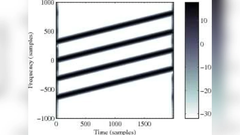
The authors develop explicit constructions for many operator pairs in one and two dimensions. In one dimension they focus on four representative non‑commuting operators: (i) time‑frequency B₁=μt+iν∂ₜ, (ii) time‑scale B₂=μt+iν(t∂ₜ+½), (iii) frequency‑scale B₃=iμ∂ₜ+iν(t∂ₜ+½), and (iv) time‑conformal B₄=μt+iν(t²∂ₜ+t). For each B_i they solve the eigenvalue problem B_i ψ_i= X ψ_i, obtaining closed‑form eigenfunctions ψ_i(μ,ν,t,X) that are essentially chirped exponentials (or scaled versions thereof). Substituting these eigenfunctions into the definition of the tomogram yields simple integral formulas such as

M₁(μ,ν,X)=\frac{1}{2π|ν|}\Big|\int_{-\infty}^{\infty} e^{i\left(\frac{μt^{2}}{2ν}-\frac{tX}{ν}\right)} f(t),dt\Big|^{2},

and analogous expressions for M₂, M₃, M₄. The parameters μ and ν control the orientation and scaling of the sampling line (or curve) in the time‑frequency plane; varying them sweeps the entire plane, much like the classical Radon transform but now along non‑linear manifolds dictated by the underlying non‑commuting algebra.

In two dimensions the construction is extended by taking independent operator pairs for each coordinate, e.g. B₁=μ₁t₁+ν₁∂{t₁}, B₂=μ₂t₂+ν₂∂{t₂}. The resulting tomogram

M(𝑿,μ,ν)=\frac{1}{(2π)^{2}|ν₁ν₂|}\Big|\iint f(t₁,t₂),e^{i\left(\frac{μ₁t₁^{2}}{2ν₁}-\frac{t₁X₁}{ν₁}+\frac{μ₂t₂^{2}}{2ν₂}-\frac{t₂X₂}{ν₂}\right)}dt₁dt₂\Big|^{2}

provides a full sampling of the four‑dimensional phase space (t₁,t₂,X₁,X₂). By imposing a linear constraint X₁+X₂=Y one obtains a “center‑of‑mass” tomogram that isolates the overall energy centroid of the signal.

A significant theoretical contribution is the embedding of tomograms into the quantizer‑dequantizer (star‑product) formalism. For any operator  one defines a symbol f_A(x)=Tr