Localization from Incomplete Noisy Distance Measurements

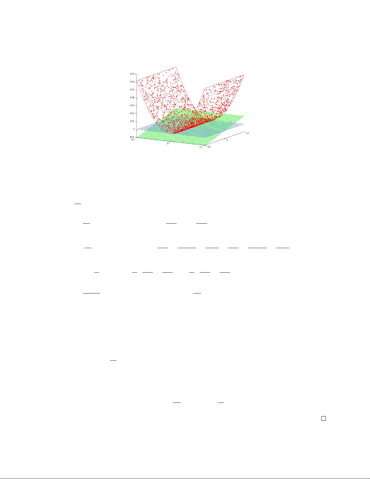
Lo calization from Incomplete Noisy Distance Measuremen ts Adel Ja v anmard ∗ Andrea Mon tanari ∗ † Abstract W e consider the problem of p ositioning a cloud of p oin ts in the Euclidean space R d , using noisy measuremen ts of a subset of pairwise distances. This task has applications in v arious areas, suc h as sensor net work lo calization and reconstruction of protein conformations from NMR measuremen ts. Also, it is closely related to dimensionality reduction problems and manifold learning, where the goal is to learn the underlying global geometry of a data set using lo cal (or partial) metric information. Here we prop ose a reconstruction algorithm based on semideﬁnite programming. F or a random geometric graph mo del and uniformly b ounded noise, we provide a precise c haracterization of the algorithm’s performance: In the noiseless case, we ﬁnd a radius r 0 b ey ond whic h the algorithm reconstructs the exact p ositions (up to rigid transformations). In the presence of noise, we obtain upp er and lo wer b ounds on the reconstruction error that matc h up to a factor that depends only on the dimension d , and the av erage degree of the no des in the graph. 1 In tro duction 1.1 Problem Statement Giv en a set of n no des in R d , the lo c alization problem requires to reconstruct the p ositions of the no des from a set of pairwise measurements ˜ d ij for ( i, j ) ∈ E ⊆ { 1 , . . . , n } × { 1 , . . . , n } . An instance of the problem is therefore giv en by the graph G = ( V , E ), V = { 1 , . . . , n } , and the vector of distance measurements ˜ d ij asso ciated to the edges of this graph. In this pap er we consider the random geometric graph mo del G ( n, r ) = ( V , E ) whereb y the n no des in V are indep enden t and uniformly random in the d -dimensional h yp ercube [ − 0 . 5 , 0 . 5] d , and E ∈ V × V is a set of edges that connect the no des which are close to each other. More sp eciﬁcally w e let ( i, j ) ∈ E if and only if d ij = k x i − x j k ≤ r . F or each edge ( i, j ) ∈ E , ˜ d ij denotes the measured distance b et ween nodes i and j . Letting z ij ≡ ˜ d 2 ij − d 2 ij the measurement error, w e will study a “worst c ase mo del” , in which the errors { z ij } ( i,j ) ∈ E are arbitrary but uniformly b ounded | z ij | ≤ ∆. W e prop ose an algorithm for this problem based on semideﬁnite programming and pro vide a rigorous analysis of its p erformance, fo cusing in particular on its robustness prop erties. Notice that the p ositions of the no des can only b e determined up to rigid transformations (a com bination of rotation, reﬂection and translation) of the no des, b ecause the inter p oint distances are inv ariant to rigid transformations. F or future use, we in tro duce a formal deﬁnition of rigid transformation. Let X ∈ R n × d b e the matrix whose i th ro w, x T i ∈ R d , is the co ordinate of no de i . F urther, let O ( d ) denote the orthogonal group of d × d matrices. A set of p ositions Y ∈ R n × d is a ∗ Departmen t of Electrical Engineering, Stanford Univ ersity † Departmen t of Statistics, Stanford Universit y 1 rigid transform of X , if there exists a d -dimensional shift vector s ∈ R d and an orthogonal matrix O ∈ O ( d ) such that Y = X O + us T . (1) Throughout u ∈ R n is the all-ones vector. Therefore, Y is obtained as a result of ﬁrst rotating (and/or reﬂecting) no des in p osition X b y matrix O and then shifting b y s . Also, tw o p osition matrices X and Y are called equiv alent up to rigid transformation, if there exists O ∈ O ( d ) and a shift s ∈ R d suc h that Y = X O + us T . W e use the following metric, similar to the one deﬁned in [16], to ev aluate the distance b et ween the original p osition matrix X ∈ R n × d and the estimation b X ∈ R n × d . Let L = I − (1 /n ) uu T b e the centering matrix . Note that L is an n × n symmetric matrix of rank n − 1 whic h eliminates the contribution of the translation, in the sense that LX = L ( X + us T ) for all s ∈ R d . F urthermore, LX X T L is in v ariant under rigid transformation and LX X L = L b X b X T L implies that X and b X are equal up to rigid transformation. The metric is deﬁned as d ( X , b X ) ≡ 1 n 2 k LX X T L − L b X b X T L k 1 . (2) This is a measure of the a verage reconstruction error p er p oin t, when X and b X are aligned optimally . T o get a b etter intuition ab out this metric, consider the case in which all the entries of LX X T L − L b X b X T L are roughly of the same order. Then d ( X , b X ) ≈ d 2 ( X , b X ) = 1 n k LX X T L − L b X b X T L k F . Denote b y Y = b X − X the estimation error, and assume without loss of generalit y that b oth X and b X are cen tered. Then for small Y , w e hav e d 2 ( X , b X ) = 1 n k X Y T + Y X T + Y Y T k F ≈ 1 n k X Y T + Y X T k F ( a ) ≥ C √ n k Y k F = C ( 1 n n X i =1 k b x i − x i k 2 ) 1 / 2 , where the b ound( a ) holds with high probability for a suitable constant C , if X is distributed according to our mo del. 1 Remark. Clearly , connectivit y of G is a necessary assumption for the lo calization problem to be solv able. It is a well kno wn result that the graph G ( n, r ) is connected w.h.p. if K d r d > (log n + c n ) /n , where K d is the v olume of the d -dimensional unit ball and c n → ∞ [18]. Vice versa, the graph is disconnected with p ositiv e probability if K d r d ≤ (log n + C ) /n for some constan t C . Hence, we fo cus on the regime where r ≥ α (log n/n ) 1 /d for some constan t α . W e further notice that, under the random geometric graph mo del, the conﬁguration of the p oin ts is almost surely generic , in the sense that the co ordinates do not satisfy any nonzero p olynomial equation with integer coeﬃcients. 1.2 Algorithm and main results The following algorithm uses semideﬁnite programming (SDP) to solve the localization problem. 1 Estimates of this type will b e rep eatedly prov ed in the following . 2 Algorithm SDP-based Algorithm for Lo calization Input: dimension d , distance measuremen ts ˜ d ij for ( i, j ) ∈ E , b ound on the measurement noise ∆ Output: estimated co ordinates in R d 1: Solv e the follo wing SDP problem: minimize T r( Q ) s.t.    h M ij , Q i − ˜ d ij 2    ≤ ∆ , ( i, j ) ∈ E Q  0 . 2: Compute the best rank- d approximation U d Σ d U T d of Q 3: Return b X = U d Σ 1 / 2 d . Here M ij = e ij e T ij ∈ R n × n , where e ij ∈ R n is the v ector with +1 at i th p osition, − 1 at j th p osition and zero ev erywhere else. Also, h A, B i ≡ T r( A T B ). Note that with a sligh t abuse of notation, the solution of the SDP problem in the ﬁrst step is denoted b y Q . Let Q 0 := X X T b e the Gram matrix of the no de p ositions, namely Q 0 ,ij = x i · x j . A k ey observ ation is that Q 0 is a lo w rank matrix: rank( Q 0 ) ≤ d , and ob eys the constraints of the SDP problem. By minimizing T r( Q ) in the ﬁrst step, w e promote low-rank solutions Q (since T r( Q ) is the sum of the eigenv alues of Q ). Alternativ ely , this minimization can b e interpreted as setting the cen ter of gra vity of { x 1 , . . . , x n } to coincide with the origin, th us removing the degeneracy due to translational inv ariance. In step 2, the algorithm computes the eigen-decomp osition of Q and retains the d largest eigen v alues. This is equiv alent to computing the b est rank- d appro ximation of Q in F rob enius norm. The center of gra vity of the reconstructed p oints remains at the origin after this op eration. Our main result provides a c haracterization of the robustness prop erties of the SDP-based algorithm. Here and below ‘with high probabilit y (w.h.p.)’ means with probabilit y conv erging to 1 as n → ∞ for d ﬁxed. Theorem 1.1. L et { x 1 , . . . , x n } b e n no des distribute d uniformly at r andom in the hyp er cub e [ − 0 . 5 , 0 . 5] d . F urther, assume c onne ctivity r adius r ≥ α (log n/n ) 1 /d , with α ≥ 10 √ d . Then w.h.p., the err or distanc e b etwe en the estimate b X r eturne d by the SDP-b ase d algorithm and the c orr e ct c o or dinate matrix X is upp er b ounde d as d ( X , b X ) ≤ C 1 ( nr d ) 5 ∆ r 4 . (3) Conversely, w.h.p., ther e exist adversarial me asur ement err ors { z ij } ( i,j ) ∈ E such that d ( X , b X ) ≥ C 2 min { ∆ r 4 , 1 } , (4) Her e, C 1 and C 2 denote universal c onstants that dep end only on d . The pro of of this theorem relies on several technical results of indep enden t interest. First, we will prov e a general deterministic error estimate in terms of the condition num b er of the stress matrix of the graph G , see Theorem 5.1. Next we will use probabilistic argumen ts to con trol the stress matrix of random geometric graphs, see Theorem 5.2. Finally , we will pro ve sev eral estimates on the rigidit y matrix of G , cf. in particular Theorem 6.1. The necessary bac kground in rigidity theory is summarized in Section 2.1. 3 1.3 Related work The lo calization problem and its v ariants ha ve attracted signiﬁcant in terest o ver the past y ears due to their applications in numerous areas, such as sensor netw ork lo calization [6], NMR sp ec- troscop y [14], and manifold learning [19, 23], to name a few. Of particular in terest to our work are the algorithms prop osed for the lo calization problem [16, 21, 6, 24]. In general, few p erformance guarantees hav e b een prov ed for these algorithms, in particular in the presence of noise. The existing algorithms can b e categorized in to t wo groups. The ﬁrst group consists of algo- rithms who try ﬁrst to estimate the missing distances and then use MDS to ﬁnd the p ositions from the reconstructed distance matrix [16, 10]. MDS-MAP [10] and ISOMAP [23] are t w o w ell-known examples of this class where the missing en tries of the distance matrix are appro ximated by com- puting the shortest paths b et ween all pairs of no des. The algorithms in the second group formulate the lo calization problem as a non-conv ex optimization problem and then use diﬀerent relaxation sc hemes to solv e it. An example of this t yp e is relaxation to an SDP [6, 22, 25, 1, 24]. A crucial assumption in these w orks is the existence of some anchors among the no des whose exact p ositions are kno wn. The SDP is then used to eﬃciently c heck whether the graph is uniquely d -lo calizable and to ﬁnd its unique realization. Maxim um V ariance Unfolding (MVU) is an SDP-based algorithm with a very similar ﬂa v or as ours [24]. MVU is an approac h to solving dimensionality reduction problems using lo cal metric information and is based on the following simple in terpretation. Assume n p oin ts lying on a low dimensional manifold in a high dimensional ambien t space. In order to ﬁnd a lo w dimensional represen tation of this data set, the algorithm attempts to somehow unfold the underlying manifold. T o this end, MVU pulls the p oin ts apart in the ambien t space, maximizing the total sum of their pairwise distances, while resp ecting the lo cal information. Ho wev er, to the b est of our kno wledge, no p erformance guarantee has b een prov ed for the MVU algorithm. Giv en the large num b er of applications, and computational metho ds developed in this broad area, the present pap er is in man y resp ects a ﬁrst step. While we focus on a sp eciﬁc mo del, and a relativ ely simple algorithm, w e exp ect that the techniques developed here will b e applicable to a broader setting, and to a n umber of algorithms in the same class. 1.4 Organization of the pap er The remainder of this pap er is organized as follo ws. Section 2 is a brief review of some notions in rigidit y theory and some prop erties of G ( n, r ) which will b e useful in this pap er. In Section 3, we discuss the implications of Theorem 1.1 in diﬀerent applications. The pro of of Theorem 1.1 (upp er b ound) is given in Section 4. Sections 5 and 6 contain the pro of of tw o imp ortan t lemmas used in proving Theorem 1.1. Sev eral technical steps are discussed in App endices. Finally , W e prov e Theorem 1.1 (lo w er b ound) in Section 7. F or the reader’s conv enience, an o verview of the symbols used throughout this pap er is given in T able 1 in App endix N. 4 2 Preliminaries 2.1 Rigidit y Theory Rigidit y theory studies whether a given partial set of pairwise distances d ij = k x i − x j k b et ween a ﬁnite set of no des in R d uniquely determine the co ordinates of the p oints up to rigid transformations. This section is a very brief ov erview of deﬁnitions and results in rigidity theory which will b e useful in this paper. W e refer the interested reader to [13, 2], for a thorough discussion. A fr amework G X in R d is an undirected graph G = ( V , E ) along with a c onﬁgur ation X ∈ R n × d whic h assigns a p oin t x i ∈ R d to each vertex i of the graph. The edges of G corresp ond to the distance constraints. In the following, we discuss tw o imp ortant notions, namely Rigidity matrix and Stress matrix. As mentioned ab o v e, a crucial part of the pro of of Theorem 1.1 consists in establishing some properties of the stress matrix and of the rigidit y matrix of the random geometric graph G ( n, r ). Rigidit y matrix. Consider a motion of the framew ork with x i ( t ) b eing the p osition vector of p oin t i at time t . Any smo oth motion that instan taneously preserv es the distance d ij m ust satisfy d dt k x i − x j k 2 = 0 for all edges ( i, j ). Equiv alen tly , ( x i − x j ) T ( ˙ x i − ˙ x j ) = 0 ∀ ( i, j ) ∈ E , (5) where ˙ x i is the v elo cit y of the i th p oin t. Given a framew ork G X ∈ R d , a solution ˙ X = [ ˙ x T 1 ˙ x T 2 · · · ˙ x T n ] T , with ˙ x i ∈ R d , for the linear system of equations (5) is called an inﬁnitesimal motion of the frame- w ork G X . This linear system of equations consists of | E | equations in dn unknowns and can b e written in the matrix form R G ( X ) ˙ X = 0, where R G ( X ) is called the | E | × dn rigidity matrix of G X . It is easy to see that for every anti-symmetric matrix A ∈ R d × d and for every vector b ∈ R d , ˙ x i = Ax i + b is an inﬁnitesimal motion. Notice that these motions are the deriv ativ e of rigid transformations. ( A corresp onds to orthogonal transformations and b corresp onds to translations). F urther, these motions span a d ( d + 1) / 2 dimensional subspace of R dn , accoun ting d ( d − 1) / 2 degrees of freedom for orthogonal transformations (corresp onding to the choice of A ), and d degrees of freedom for translations (corresp onding to the choice of b ). Hence, dim Ker( R G ( X )) ≥ d ( d + 1) / 2. A framework is said to b e inﬁnitesimal ly rigid if dim Ker( R G ( X )) = d ( d + 1) / 2. Stress matrix. A str ess for a framework G X is an assignment of scalars ω ij to the edges such that for eac h i ∈ V , X j :( i,j ) ∈ E ω ij ( x i − x j ) = ( X j :( i,j ) ∈ E ω ij ) x i − X j :( i,j ) ∈ E ω ij x j = 0 . A stress vector can b e rearranged into an n × n symmetric matrix Ω , known as the str ess matrix , suc h that for i 6 = j , the ( i, j ) entry of Ω is Ω ij = − ω ij , and the diagonal entries for ( i, i ) are Ω ii = P j : j 6 = i ω ij . Since all the co ordinate vectors of the conﬁguration as w ell as the all-ones vector are in the n ull space of Ω, the rank of the stress matrix for generic conﬁgurations is at most n − d − 1. There is an imp ortan t relation b etw een stress matrices of a framework and the notion of glob al rigidity . A framew ork G X is said to be glob al ly rigid in R d if all framew orks in R d with the same set of edge lengths are congruen t to G X , i.e. are a rigid transformation of G X . F urther, a framework G X is generic al ly glob al ly rigid in R d if G X is globally rigid at all generic conﬁgurations X . (Recall 5 that a conﬁguration of p oin ts is called generic if the co ordinates of the p oin ts do not satisfy an y nonzero p olynomial equation with in teger coeﬃcients). The connection b et ween global rigidit y and stress matrices is demonstrated in the following t wo results prov ed in [9] and [13]. Theorem 2.1 (Connelly , 2005) . If X is a generic c onﬁgur ation in R d with a str ess matrix Ω of r ank n − d − 1 , then G X is glob al ly rigid in R d . Theorem 2.2 (Gortler, Healy , Thurston, 2010) . Supp ose that X is a generic c onﬁgur ation in R d , such that G X is glob al ly rigid in R d . Then either G X is a simplex or it has a str ess matrix Ω with r ank n − d − 1 . Among other results in this pap er, we construct a sp ecial stress matrix Ω for the random geometric graph G ( n, r ). W e also provide upp er b ound and low er b ound on the maximum and the minimum nonzero singular v alues of this stress matrix. These b ounds are used in proving Theorem 1.1. 2.2 Some Prop erties of G ( n, r ) In this section, w e study some of the basic prop erties of G ( n, r ) whic h will b e used sev eral times throughout the paper. Our ﬁrst remark pro vides probabilistic b ounds on the num b er of no des con tained in a region R ⊆ [ − 0 . 5 , 0 . 5] d . Remark 2.1.[Sampling Lemma] Let R b e a measurable subset of the h yp ercub e [ − 0 . 5 , 0 . 5] d , and let V ( R ) denote its volume. Assume n no des are deploy ed uniformly at random in [ − 0 . 5 , 0 . 5] d , and let n ( R ) b e the num b er of no des in region R . Then, n ( R ) ∈ nV ( R ) + [ − p 2 cnV ( R ) log n, p 2 cnV ( R ) log n ] , (6) with probability at least 1 − 2 /n c . The pro of is immediate and deferred to App endix A. In the graph G ( n, r ), every no de is connected to all the no des within its r -neigh b orho od. Using Remark 2.1 for r -neigh b orhoo d of each no de, and the fact r ≥ 10 √ d (log n/n ) 1 /d , we obtain the follo wing corollary after applying union b ound ov er all the r -neigh b orhoo ds of the no des. Corollary 2.1. In the gr aph G ( n, r ) , with r ≥ 10 √ d (log n/n ) 1 /d , the de gr e es of al l no des ar e in the interval [(1 / 2) K d nr d , (3 / 2) K d nr d ] , with high pr ob ability. Her e, K d is the volume of the d -dimensional unit b al l. Next, we discuss some properties of the sp ectrum of G ( n, r ). Recall that the Laplacian L of the graph G is the symmetric matrix indexed by the vertices V , such that L ij = − 1 if ( i, j ) ∈ E , L ii = degree( i ) and L ij = 0 otherwise. The all-ones vector u ∈ R n is an eigenv ector of L ( G ) with eigen v alue 0. F urther, the multiplicit y of eigen v alue 0 in sp ectrum of L ( G ) is equal to the num be r of connected comp onen ts in graph G . Let us stress that our deﬁnition of L ( G ) has opp osite sign with resp ect to the one adopted b y part of the computer science literature. In particular, with the present deﬁnition, L ( G ) is a p ositiv e semideﬁnite matrix. It is useful to recall a basic estimate on the Laplacian of random geometric graphs. 6 Remark 2.2. Let L n denote the normalized Laplacian of the random geometric graph G ( n, r ), deﬁned as L n = D − 1 / 2 L D − 1 / 2 , where D is the diagonal matrix with degrees of the no des on diagonal. Then, w.h.p., λ 2 ( L n ), the second smallest eigenv alue of L n , is at least C r 2 ([7, 18]). Also, using the result of [8] (Theorem 4) and Corollary 2.1, we ha v e λ 2 ( L ) ≥ C ( nr d ) r 2 , for some constant C = C ( d ). 2.3 Notations F or a vector v ∈ R n , and a subset T ⊆ { 1 , · · · , n } , v T ∈ R T is the restriction of v to indices in T . W e use the notation h v 1 , · · · , v n i to represent the subspace spanned b y v ectors v i , 1 ≤ i ≤ n . The orthogonal pro jections onto subspaces V and V ⊥ are resp ectiv ely denoted b y P V and P ⊥ V . The iden tity matrix, in any dimension, is denoted by I . F urther, e i alw ays refers to the i th standard basis elemen t, e.g., e 1 = (1 , 0 , · · · , 0). Throughout this paper, u ∈ R n is the all-ones v ector and C is a constan t dep ending only on the dimension d , whose v alue may change from case to case. Giv en a matrix A , we denote its op erator norm b y k A k 2 , its F rob enius norm b y k A k F , its n uclear norm by k A k ∗ , and its ` 1 -norm b y k A k 1 . ( k A k ∗ is simply the sum of the singular v alues of A and k A k 1 = P ij | A ij | ). W e also use σ max ( A ) and σ min ( A ) to respectively denote the maximum and the minim um nonzero singular v alues of A . F or a graph G , w e denote by V ( G ) the set of its vertices and w e use E ( G ) to denote the set of edges in G . F ollowing the con ven tion adopted abov e, the Laplacian of G is represented by L ( G ). Finally , we denote b y x ( i ) ∈ R n , i ∈ { 1 , . . . , d } the i th column of the p ositions matrix X . In other words x ( i ) is the v ector containing the i th co ordinate of p oin ts x 1 , . . . , x n . Throughout the pro of w e shall adopt the con ven tion of using the notations X , { x j } j ∈ [ n ] , and { x ( i ) } i ∈ [ d ] to denote the centered positions. In other words X = LX 0 where the rows of X 0 are i.i.d. uniform in [ − 0 . 5 , 0 . 5] d . 3 Discussion In this section, w e mak e some remarks ab out Theorem 1.1 and its implications. Tigh tness of the Bounds. The upp er and the lo wer b ounds in Theorem 1.1 matc h up to the factor C ( nr d ) 5 . Note that nr d is the av erage degree of the no des in G (up to a constan t) and when the rang r is of the same order as the connectivity threshold, i.e., r = O ((log n/n ) 1 /d ), it is logarithmic in n . F urthermore, we b eliev e that this factor is the artifact of our analysis. The n umerical exp eriments in Section 8 also supp ort the idea that the p erformance of the SDP-based algorithm, ev aluated b y d ( X , b X ), scales as C ∆ /r 4 for some constan t C . In addition, the theorem states the b ounds for r ≥ α (log n/n ) 1 /d , with α ≥ 10 √ d . How ev er, n umerical exp erimen ts in Section 8 show that the b ounds hold for m uch smaller α , namely α ≥ 3 for d = 2 , 4. Finally , it is immediate to see that under the worst case mo del for the measuremen t errors, no algorithm can perform b etter than C ∆ /r 2 . More speciﬁcally , for an y algorithm d ( X , b X ) ≥ C ∆ /r 2 , for some constan t C . The reason is that letting ˜ d ij 2 = (1 + ∆ /r 2 ) d 2 ij , no algorithm can diﬀerentiate b et ween X and its scaled v ersion b X = p 1 + ∆ /r 2 X . Also d ( X , b X ) = (∆ /r 2 )(1 /n 2 ) k LX X T L k 1 ≥ C ∆ /r 2 , w.h.p. and for some constan t C that dep ends on the dimension d . Global Rigidity of G ( n, r ) . As a special case of Theorem 1.1 we can consider the problem of reconstructing the p oin t p ositions from exact measurements. The case of exact measurements was 7 also studied recently in [20] following a diﬀerent approac h. This corresp onds to setting ∆ = 0. The underlying question is whether the p oin t p ositions { x i } i ∈ V can b e eﬃcien tly determined (up to a rigid motion) by the set of distances { d ij } ( i,j ) ∈ E . If this is the case, then, in particular, the random graph G ( n, r ) is globally rigid. Since the right-hand side of our error b ound Eq. (3) v anishes for ∆ = 0, we immediately obtain the following. Corollary 3.1. L et { x 1 , . . . , x n } b e n no des distribute d uniformly at r andom in the hyp er cub e [ − 0 . 5 , 0 . 5] d . If r ≥ 10 √ d (log n/n ) 1 /d , and the distanc e me asur ements ar e exact, then w.h.p., the SDP-b ase d algorithm r e c overs the exact p ositions (up to rigid tr ansformations). In p articular, the r andom ge ometric gr aph G ( n, r ) is w.h.p. globally rigid if r ≥ 10 √ d (log n/n ) 1 /d . In [3], the authors prov e a similar result on global rigidity of G ( n, r ). Namely , they sho w that if n p oin ts are drawn from a P oisson pro cess in [0 , 1] 2 , then the random geometric graph G ( n, r ) is globally rigid w.h.p. when r is of the order p log n/n . As already men tioned ab ov e, the graph G ( n, r ) is disconnected with high probabilit y if r ≤ K − 1 /d d ((log n + C ) /n ) 1 /d for some constant C . Hence, our result establishes the follo wing rigidity phase tr ansition phenomenon: There exist dimension-dependent constan ts C 1 ( d ), C 2 ( d ) suc h that a random geometric graph G ( n, r ) is with high probabilit y not globally rigid if r ≤ C 1 ( d )(log n/n ) 1 /d , and with high probability globally rigid if r ≥ C 2 ( d )(log n/n ) 1 /d . Applying Stirling formula, it is easy to see that the abov e argumen ts yield C 1 ( d ) ≥ C 1 , ∗ √ d and C 2 ( d ) ≤ C 2 , ∗ √ d for some numerical (dimension indep enden t) constan ts C 1 , ∗ , C 2 , ∗ . It is natural to conjecture that the rigidity phase transition is sharp. Conjecture 1. L et G ( n, r n ) b e a r andom ge ometric gr aph with n no des, and r ange r n , in d dimensions. Then ther e exists a c onstant C ∗ ( d ) such that, for any ε > 0 , the fol lowing hap- p ens. If r n ≤ ( C ∗ ( d ) − ε )(log n/n ) 1 /d , then G ( n, r n ) is with high pr ob ability not glob al ly rigid. If r n ≥ ( C ∗ ( d ) + ε )(log n/n ) 1 /d , then G ( n, r n ) is with high pr ob ability glob al ly rigid. Sensor Net work Lo calization. Research in this area aims at developing algorithms and systems to determine the p ositions of the no des of a sensor netw ork exploiting inexp ensiv e distributed measuremen ts. Energy and hardware constrain ts rule out the use of global p ositioning systems, and several prop osed systems exploit pairwise distance measurements b et ween the sensors [17, 15]. These techniques ha v e acquired new industrial interest due to their relev ance to indo or p ositioning. In this con text, global p ositioning systems are not a metho d of c hoice b ecause of their limited accuracy in indoor en vironments. Semideﬁnite programming metho ds for sensor netw ork lo calization hav e b een dev elop ed starting with [6]. It is common to study and ev aluate diﬀerent tec hniques within the random geometric graph mo del, but no p erformance guaran tees hav e b een prov en for adv anced (SDP based) algorithms, with inaccurate measurements. W e shall therefore consider n sensors placed uniformly at random in the unit hypercub e, with ambien t dimension either d = 2 or d = 3 dep ending on the sp eciﬁc application. The connectivity range r is dictated by v arious factors: pow er limitations; interference b et w een nearb y no des; loss of accuracy with distance. The measurement error z ij dep ends on the metho d used to measure the distance b et ween nodes i and j . W e will limit ourselves to measurement errors due to noise (as opp osed –for instance– to malicious b eha vior of the no des) and discuss tw o common tec hniques for measuring distances 8 b et w een wireless devices: Receiv ed Signal Indicator (RSSI) and Time Diﬀerence of Arriv al (TDoA). RSSI measures the ratio of the p o wer present in a received radio signal ( P r ) and a reference transmitted p ow er ( P s ). The ratio P r /P s is inv ersely prop ortional to the square of the distance b et w een the receiver and the transmitter. Hence, RSSI can b e used to estimate the distance. It is reasonable to assume that the dominant error is in the measurement of the receiv ed pow er, and that it is prop ortional to the transmitted p o wer. W e th us assume that there is an error ε P s in measuring the received pow er P r ., i.e., e P r = P r + ε P s , where e P r denotes the measured received p o w er. Then, the measured distance is given by ˜ d 2 ij ∝ P s ˜ P r = P s P r ·  1 + P s P r ε  − 1 ≈ P s P r  1 − P s P r ε  ∝ d 2 ij (1 − C d 2 ij ε ) . (7) Therefore the o verall error | z ij | ∝ d 4 ij ε and its magnitude is ∆ ∝ r 4 ε . Applying Theorem 1.1, we obtain an a v erage error p er no de of order d ( X , b X ) ≤ C 0 1 ( nr d ) 5 ε . In other w ords, the p ositioning accuracy is linear in the measuremen t accuracy , with a propor- tionalit y constan t that is p olynomial in the av erage no de degree. Remark ably , the b est accuracy is obtained by using the smallest av erage degree, i.e. the smallest measuremen t radius that is compatible with connectivit y . TDoA tec hnique uses the time diﬀerence b et ween the receipt of tw o diﬀerent signals with diﬀeren t v elo cities, for instance ultrasound and radio signals. The time diﬀerence is prop ortional to the distance betw een the receiver and the transmitter, and given the v elo cit y of the signals the distance can b e estimated from the time diﬀerence. Now, assume that there is a relative error ε in measuring this time diﬀerence (this migh t b e related to inaccuracies in ultrasound sp eed). W e th us ha ve e t ij = t ij (1 + ε ), where e t ij is the measured time while t ij is the ‘ideal’ time diﬀerence. This leads to an error in estimating d ij whic h is prop ortional to d ij ε . Therefore, | z ij | ∝ d 2 ij ε and ∆ ∝ r 2 ε . Applying again Theorem 1.1, we obtain an av erage error per node of order d ( X , b X ) ≤ C 0 1 ( nr d ) 5 ε r 2 . In other words the reconstruction error decreases with the measuremen t radius, whic h suggests somewhat diﬀerent net work design for suc h a system. Let us stress in passing that the abov e error bounds are pro v ed under an adv ersarial error model (see b elo w). It would b e useful to complemen t them with similar analysis carried out for other, more realistic, models. Manifold Learning. Manifold learning deals with ﬁnite data sets of points in am bient space R N whic h are assumed to lie on a smo oth submanifold M d of dimension d < N . The task is to recov er M given only the data p oin ts. Here, w e discuss the implications of Theorem 1.1 for applications of SDP methods to manifold learning. It is typically assumed that the manifold M d is isometrically equiv alent to a region in R d . F or the sak e of simplicit y we shall assume that this region is con vex (see [12] for a discussion of this p oin t). With little loss of generality we can indeed identify the region with the unit h yp ercube [ − 0 . 5 , 0 . 5] d . A t ypical manifold learning algorithm ([23] and [24]) estimates the ge o desic distances b et w een a subset of pairs of data p oin ts d M ( y i , y j ), y i ∈ R N , and then tries to ﬁnd a lo w-dimensional em b edding (i.e. p ositions x i ∈ R d ) that reproduce these distances. 9 The unkno wn geo desic distance b et ween nearby data p oin ts y i and y j , denoted by d M ( y i , y j ), can b e estimated by their Euclidean distance in R n . Therefore the manifold learning problem reduces mathematically to the lo calization problem whereby the distance ‘measurements’ are ˜ d ij = k y i − y j k R N , while the actual distances are d ij = d M ( y i , y j ). The accuracy of these estimates dep ends on the curv ature of the manifold M . Let r 0 = r 0 ( M ) b e the minimum r adius of curvatur e deﬁned by: 1 r 0 = max γ ,t {k ¨ γ ( t ) k} , where γ v aries o ver all unit-sp eed geo desics in M and t is in the domain of γ . F or instance, an Euclidean sphere of radius r 0 has minimum radius of curv ature equal to r 0 . As shown in [5] (Lemma 3), (1 − d 2 ij / 24 r 2 0 ) d ij ≤ ˜ d ij ≤ d ij . Therefore, | z ij | ∝ d 4 ij /r 2 0 , and ∆ ∝ r 4 /r 2 0 . Theorem 1.1 supp orts the claim that the estimation error d ( X, b X ) is b ounded b y C ( nr d ) 5 /r 2 0 . As mentioned sev eral times, this pap er fo cuses on a particularly simple SDP relaxation, and noise mo del. This op ens the w a y to a num b er of interesting directions: 1. Sto chastic noise mo dels . A somewhat complementary direction to the one tak en here would b e to assume that the distance measurements are ˜ d 2 ij = d 2 ij + z ij with { z ij } a collection of indep enden t zero-mean random v ariables. This would b e a goo d mo del, for instance, for errors in RSSI measuremen ts. Another in teresting case would b e the one in whic h a small subset of measuremen ts are grossly incorrect (e.g. due to no de malfunctioning, obstacles, etc.). 2. Tighter c onvex r elaxations . The relaxation considered here is particularly simple, and can b e improv ed in sev eral wa ys. F or instance, in manifold learning it is useful to maximize the em b edding v ariance T r( Q ) under the constraint Qu = 0 [24]. Also, for an y pair ( i, j ) 6∈ E it is p ossible to add a constrain t of the form h M ij , Q i ≤ ˆ d 2 ij , where ˆ d ij is an upp er b ound on the distance obtained b y computing the shortest path b et w een i and j in G . 3. Mor e gener al ge ometric pr oblems . The present pap er analyzes the problem of reconstructing the geometry of a cloud of p oints from incomplete and inaccurate measurements of the p oin ts lo cal geometry . F rom this p oin t of view, a n umber of interesting extensions can b e explored. F or instance, instead of distances, it might be p ossible to measure angles b et ween edges in the graph G (indeed in sensor netw orks, angles of arriv al migh t b e a v ailable [17, 15]). 4 Pro of of Theorem 1.1 (Upp er Bound) Let V = h u, x (1) , · · · , x ( d ) i and for an y matrix S ∈ R n × n , deﬁne ˜ S = P V S P V + P V S P ⊥ V + P ⊥ V S P V , S ⊥ = P ⊥ V S P ⊥ V . (8) Th us S = ˜ S + S ⊥ . Also, denote b y R the diﬀerence b et ween the optimum solution Q and the actual Gram matrix Q 0 , i.e., R = Q − Q 0 . The pro of of Theorem 1.1 is based on the following key lemmas that bound R ⊥ and ˜ R separately . 10 Lemma 4.1. Ther e exists a numeric al c onstant C = C ( d ) , such that, w.h.p., k R ⊥ k ∗ ≤ C n r 4 ( nr d ) 5 ∆ . (9) Lemma 4.2. Ther e exists a numeric al c onstant C = C ( d ) , such that, w.h.p., k ˜ R k 1 ≤ C n 2 r 4 ( nr d ) 5 ∆ . (10) W e defer the proof of lemmas 4.1 and 4.2 to the next section. Pr o of (The or em 1.1). Let Q = P n i =1 σ i u i u T i , where k u i k = 1, u T i u j = 0 for i 6 = j and σ 1 ≥ σ 2 ≥ · · · ≥ σ n ≥ 0. Let P d ( Q ) = P d i =1 σ i u i u T i b e the best rank- d appro ximation of Q in F rob enius norm (step 2 in the algorithm). Recall that Qu = 0, b ecause Q minimizes T r( Q ). Consequently , P d ( Q ) u = 0 and P d ( Q ) = L P d ( Q ) L . F urther, b y our assumption Q 0 u = 0 and th us Q 0 = LQ 0 L . Using triangle inequalit y , k L P d ( Q ) L − LQ 0 L k 1 = kP d ( Q ) − Q 0 k 1 ≤ kP d ( Q ) − ˜ Q k 1 + k ˜ Q − Q 0 k 1 . (11) Observ e that, ˜ Q = Q 0 + ˜ R and Q ⊥ = R ⊥ . Since P d ( Q ) − ˜ Q has rank at most 3 d , it follo ws that kP d ( Q ) − ˜ Q k 1 ≤ n kP d ( Q ) − ˜ Q k F ≤ √ 3 dn kP d ( Q ) − ˜ Q k 2 (for any matrix A , k A k 2 F ≤ rank( A ) k A k 2 2 ). By triangle inequalit y , we hav e kP d ( Q ) − ˜ Q k 2 ≤ kP d ( Q ) − Q k 2 + k Q − ˜ Q | {z } R ⊥ k 2 . (12) Note that kP d ( Q ) − Q k 2 = σ d +1 . Recall the v ariational principle for the eigen v alues. σ q = min H,dim ( H )= n − q +1 max y ∈ H, k y k =1 y T Qy . T aking H = h x (1) , · · · , x ( d ) i ⊥ , for an y y ∈ H , y T Qy = y T P ⊥ V QP ⊥ V y = y T Q ⊥ y = y T R ⊥ y , where we used the fact Qu = 0 in the ﬁrst equality . Therefore, σ d +1 ≤ max k y k =1 y T R ⊥ y = k R ⊥ k 2 It follo ws from Eqs. (11) and (12) that k L P d ( Q ) L − LQ 0 L k 1 ≤ 2 √ 3 dn k R ⊥ k 2 + k ˜ R k 1 . Using Lemma 4.1 and 4.2, w e obtain d ( X , b X ) = 1 n 2 k L P d ( Q ) L − LQ 0 L k 1 ≤ C ( nr d ) 5 ∆ r 4 , whic h pro ves the claimed upp er b ound on the error. The low er b ound is pro ved in Section 7. 11 5 Pro of of Lemma 4.1 The pro of is based on the following three steps: ( i ) Upp er bound k R ⊥ k ∗ in terms of σ min (Ω) and σ max (Ω), where Ω is an arbitrary p ositive semideﬁnite (PSD) stress matrix of rank n − d − 1 for the framew ork; ( ii ) Construct a particular PSD stress matrix Ω of rank n − d − 1 for the framework; ( iii ) Upp er b ound σ max (Ω) and lo w er b ound σ min (Ω). Theorem 5.1. L et Ω b e an arbitr ary PSD str ess matrix for the fr amework G X such that rank(Ω) = n − d − 1 . Then, k R ⊥ k ∗ ≤ 2 σ max (Ω) σ min (Ω) | E | ∆ . (13) Pr o of. Note that R ⊥ = Q ⊥ = P ⊥ V QP ⊥ V  0 . W rite R ⊥ = P n − d − 1 i =1 λ i u i u T i , where k u i k = 1, u T i u j = 0 for i 6 = j and λ 1 ≥ λ 2 ≥ · · · λ n − d − 1 ≥ 0. Therefore, h Ω , R ⊥ i = h Ω , n − d − 1 X i =1 λ i u i u T i i = n − d − 1 X i =1 λ i u T i Ω u i ≥ σ min (Ω) k R ⊥ k ∗ . (14) Here, we used the fact that u i ∈ V ⊥ = Ker ⊥ (Ω). Note that σ min (Ω) > 0, since Ω  0 . No w, w e need to upp er b ound the quan tity h Ω , R ⊥ i . Since Ω u = 0, the stress matrix Ω = [ ω ij ] can b e written as Ω = P ( i,j ) ∈ E ω ij M ij . Deﬁne ω max = max i 6 = j | ω ij | . Then, h Ω , R ⊥ i ( a ) = h Ω , R i = X ( i,j ) ∈ E ω ij h M ij , R i ≤ X ( i,j ) ∈ E ω max |h M ij , Q − Q 0 i| ≤ X ( i,j ) ∈ E ω max ( |h M ij , Q i − ˜ d ij 2 | + | ˜ d ij 2 − d 2 ij | {z } z ij | ) ≤ 2 ω max | E | ∆ , (15) where ( a ) follows from the fact that h P V , Ω i = 0. Since Ω  0 , w e ha ve ω 2 ij ≤ ω ii ω j j = ( e T i Ω e i )( e T j Ω e j ) ≤ σ 2 max (Ω), for 1 ≤ i, j ≤ n . Hence, ω max ≤ σ max (Ω). Combining Eqs. (14) and (15), w e get the desired result. Next step is constructing a PSD stress matrix of rank n − d − 1. F or each no de i ∈ V ( G ) deﬁne C i = { j ∈ V ( G ) : d ij ≤ r / 2 } . Note that the nodes in each C i form a clique in G . In addition, let S i b e the following set of cliques. S i := ∪ k ∈C i {C i \ k } ∪ {C i } . Therefore, S i is a set of |C i | + 1 cliques. F or the graph G , we deﬁne cliq ( G ) := S 1 ∪ · · · ∪ S n . Next lemma establishes a simple prop erty of cliques C i . Its pro of is immediate and deferred to App endix B. Prop osition 5.1. If r ≥ 4 c √ d (log n/n ) 1 /d with c > 1 , the fol lowing is true w.h.p.. F or any two no des i and j , such that k x i − x j k ≤ r / 2 , |C i ∩ C j | ≥ d + 1 . 12 No w w e are ready to construct a special stress matrix Ω of G X . Deﬁne the |Q k | × |Q k | matrix Ω k as follows. Ω k = P ⊥ h u Q k ,x (1) Q k , ··· ,x ( d ) Q k i . Let ˆ Ω k b e the n × n matrix obtained from Ω k b y padding it with zeros. Deﬁne Ω = X Q k ∈ cliq ( G ) ˆ Ω k . The pro of of the next statement is again immediate and discussed in App endix C. Prop osition 5.2. The matrix Ω deﬁne d ab ove is a p ositive semideﬁnite (PSD) str ess matrix for the fr amework G X . F urther, almost sur ely, rank(Ω) = n − d − 1 . Final step is to upp er b ound σ max (Ω) and lo w er b ound σ min (Ω). Claim 5.1. Ther e exists a c onstant C = C ( d ) , such that, w.h.p., σ max (Ω) ≤ C ( nr d ) 2 . Pr o of. F or any vector v ∈ R n , v T Ω v = X Q k ∈ cliq ( G ) v T ˆ Ω k v = X Q k ∈ cliq ( G ) k ˆ Ω k v k 2 = X Q k ∈ cliq ( G ) k P ⊥ h u Q k ,x (1) Q k , ··· ,x ( d ) Q k i v Q k k 2 ≤ X Q k ∈ cliq ( G ) k v Q k k 2 = n X j =1 v 2 j X k : j ∈Q k 1 = n X j =1 ( X i ∈C j |C i | ) v 2 j ≤ ( C nr d k v k ) 2 . The last inequalit y follo ws from the fact that, w.h.p., |C j | ≤ C nr d for all j and some constant C (see Corollary 2.1). W e no w pass to low er b ounding σ min (Ω). Theorem 5.2. Ther e exists a c onstant C = C ( d ) , such that, w.h.p., Ω ⊥  C ( nr d ) − 3 r 2 L ⊥ . ( se e Eq. (8)) . The pro of is giv en in Section 5.1. W e are ﬁnally in p osition to pro ve Lemma 4.1. Pr o of (L emma 4.1). F ollo wing Theorem 5.2 and Remark 2.2, we obtain σ min (Ω) ≥ C ( nr d ) − 2 r 4 . Also, by Corollary 2.1, w.h.p., the no de degrees in G are b ounded by 3 / 2 K d nr d . Hence, w.h.p., | E | ≤ 3 / 4 n 2 K d r d . Using the b ounds on σ max (Ω), σ min (Ω) and | E | in Theorem 5.1 yields the thesis. 5.1 Pro of of Theorem 5.2 Before turning to the pro of, it is w orth mentioning that the authors in [4] prop ose a heuristic argumen t showing Ω v ≈ L 2 v for smo othly v arying vectors v . Since σ min ( L ) ≥ C ( nr d ) r 2 (see Remark 2.2), this heuristic supp orts the claim of the theorem. In the follo wing, we ﬁrst establish some claims and deﬁnitions which will b e used in the pro of. 13 Claim 5.2. Ther e exists a c onstant C = C ( d ) , such that, w.h.p., L  C n X k =1 P ⊥ u C k . The argument is closely related to the Mark ov c hain comparison technique [11]. The pro of is giv en in App endix D. The next claim provides a concen tration res ult ab out the n umber of no des in the cliques C i . Its pro of is immediate and deferred to Appendix E. Claim 5.3. F or every no de i ∈ V ( G ) , deﬁne ˜ C i = { j ∈ V ( G ) : d ij ≤ r 2 ( 1 2 + 1 100 ) } . Ther e exists an inte ger numb er m such that the fol lowing is true w.h.p.. | ˜ C i | ≤ m ≤ |C i | , ∀ i ∈ V ( G ) . No w, for any node i , let i 1 , · · · i m denote the m -nearest neighbors of that no de. Using claim 5.3, ˜ C i ⊆ { i 1 , · · · , i m } ⊆ C i . Deﬁne the set ˜ S i as follows. ˜ S i = {C i , C i \ i 1 , · · · , C i \ i m } . Therefore, ˜ S i is a set of ( m + 1) cliques. Let cliq ∗ ( G ) = ˜ S 1 ∪ · · · ∪ ˜ S n . Note that cliq ∗ ( G ) ⊆ cliq ( G ). Construct the graph G ∗ in the following wa y . F or ev ery elemen t in cliq ∗ ( G ), there is a corresp onding v ertex in G ∗ . (Thus, | V ( G ∗ ) | = n ( m + 1)). Also, for an y t wo nodes i and j , suc h that k x i − x j k ≤ r / 2, ev ery vertex in V ( G ∗ ) corresp onding to an element in ˜ S i is connected to every v ertex in V ( G ∗ ) corresp onding to an elemen t in ˜ S j . Our next claim establishes some prop erties of the graph G ∗ . F or its pro of, we refer to Ap- p endix F. Claim 5.4. With high pr ob ability, the gr aph G ∗ has the fol lowing pr op erties. ( i ) The de gr e e of e ach no de is b ounde d by C ( nr d ) 2 , for some c onstant C = C ( d ) . ( ii ) L et L ∗ denote the L aplacian of G ∗ . Then σ min ( L ∗ ) ≥ C ( nr d ) 2 r 2 , for some c onstant C . No w, w e are in p osition to pro v e Theorem 5.2 Pr o of (The or em 5.2). Let v ∈ V ⊥ b e an arbitrary v ector. F or every clique Q i ∈ cliq ( G ), de- comp ose v lo cally as v Q i = P d ` =1 β ( ` ) i ˜ x ( ` ) Q i + γ i u Q i + w ( i ) , where ˜ x ( ` ) Q i = P ⊥ u Q i x ( ` ) Q i and w ( i ) ∈ h x (1) Q i , · · · , x ( d ) Q i , u Q i i ⊥ . Hence, v T Ω v = X Q i ∈ cliq ( G ) k w ( i ) k 2 . Note that v Q i ∩Q j has t wo representations; One is obtained by restricting v Q i to indices in Q j , and the other is obtained by restricting v Q j to indices in Q i . F rom these t wo representations, we get w ( i ) Q i ∩Q j − w ( j ) Q i ∩Q j = d X ` =1 ( β ( ` ) j − β ( ` ) i ) ˜ x ( ` ) Q i ∩Q j + ˜ γ i,j u Q i ∩Q j . (16) 14 Here, ˜ x ( ` ) Q i ∩Q j = P ⊥ u Q i ∩Q j x ( ` ) Q i ∩Q j . The v alue of γ i,j do es not matter to our argumen t; how ever it can b e giv en explicitly . Note that {C 1 , · · · , C n } ⊆ cliq ∗ ( G ) ⊆ cliq ( G ). In voking Claim 5.2, v T L v ≤ C n X k =1 k P ⊥ u C k v C k k 2 ≤ C X Q i ∈ cliq ∗ ( G ) k P ⊥ u Q i v Q i k 2 = C X Q i ∈ cliq ∗ ( G )    d X ` =1 β ( ` ) i ˜ x ( ` ) Q i + w ( i )    2 = C   X Q i ∈ cliq ∗ ( G )    d X ` =1 β ( ` ) i ˜ x ( ` ) Q i    2 + X Q i ∈ cliq ∗ ( G ) k w ( i ) k 2   ≤ C   d X Q i ∈ cliq ∗ ( G ) d X ` =1    β ( ` ) i ˜ x ( ` ) Q i    2 + X Q i ∈ cliq ∗ ( G ) k w ( i ) k 2   . Hence, we only need to sho w that X Q i ∈ cliq ( G ) k w ( i ) k 2 ≥ C ( nr d ) − 3 r 2 X Q i ∈ cliq ∗ ( G ) d X ` =1    β ( ` ) i ˜ x ( ` ) Q i    2 , (17) for some constan t C = C ( d ). In the following we adopt the conv ention that for j ∈ V ( G ∗ ), Q j is the corresp onding clique in cliq ∗ ( G ). W e ha ve X Q i ∈ cliq ( G ) k w ( i ) k 2 ≥ X Q i ∈ cliq ∗ ( G ) k w ( i ) k 2 = X i ∈ V ( G ∗ ) k w ( i ) k 2 ( a ) ≥ C ( nr d ) − 2 X ( i,j ) ∈ E ( G ∗ ) ( k w ( i ) k 2 + k w ( j ) k 2 ) ≥ C ( nr d ) − 2 X ( i,j ) ∈ E ( G ∗ ) k w ( i ) Q i ∩Q j − w ( j ) Q i ∩Q j k 2 ( b ) ≥ C ( nr d ) − 2 X ( i,j ) ∈ E ( G ∗ )    d X ` =1 ( β ( ` ) j − β ( ` ) i ) ˜ x ( ` ) Q i ∩Q j    2 ( c ) ≥ C ( nr d ) − 1 r 2 X ( i,j ) ∈ E ( G ∗ ) d X ` =1 ( β ( ` ) j − β ( ` ) i ) 2 . (18) Here, ( a ) follows from the fact that the degrees of no des in G ∗ are b ounded by C ( nr d ) 2 (Claim 5.4, part ( i )); ( b ) follows from Eq. (16) and ( c ) follows from Claim 5.5, whose pro of is deferred to App endix G. Claim 5.5. Ther e exists a c onstant C = C ( d ) , such that, for any set of values { β ( ` ) i } the fol lowing holds with high pr ob ability.    d X ` =1 ( β ( ` ) j − β ( ` ) i ) ˜ x ( ` ) Q i ∩Q j    2 ≥ C ( nr d ) r 2 d X ` =1 ( β ( ` ) j − β ( ` ) i ) 2 , ∀ ( i, j ) ∈ E ( G ∗ ) . 15 Also note that k ˜ x ( ` ) Q i k 2 ≤ |Q i | r 2 and w.h.p., |Q i | ≤ C ( nr d ), for all i ∈ V ( G ∗ ) (since, w.h.p., |C i | ≤ C ( nr d ) for all i ∈ V ( G ) b y Corollary 2.1 ). Therefore, using Eq. (18), in order to pro v e (17) it suﬃces to sho w that d X ` =1 X ( i,j ) ∈ E ( G ∗ ) ( β ( ` ) j − β ( ` ) i ) 2 ≥ C ( nr d ) − 1 r 2 d X ` =1 X i ∈ V ( G ∗ ) ( β ( ` ) i ) 2 . Deﬁne β ( ` ) = ( β ( ` ) i ) i ∈ V ( G ∗ ) . Observ e that, X ( i,j ) ∈ E ( G ∗ ) ( β ( ` ) j − β ( ` ) i ) 2 = ( β ( ` ) ) T L ∗ β ( ` ) ≥ σ min ( L ∗ ) k P ⊥ u β ( ` ) k 2 . Using Claim 5.4 (part ( ii )) w e obtain X ( i,j ) ∈ E ( G ∗ ) ( β ( ` ) j − β ( ` ) i ) 2 ≥ C ( nr d ) 2 r 2 k P ⊥ u β ( ` ) k 2 . The pro of is completed b y the following claim, whose pro of is giv en in Appendix H. Claim 5.6. Ther e exists a c onstant C = C ( d ) , such that, the fol lowing holds with high pr ob ability. Consider an arbitr ary ve ctor v ∈ V ⊥ with lo c al de c omp ositions v Q i = P d ` =1 β ( ` ) i ˜ x ( ` ) Q i + γ i u Q i + w ( i ) . Then, d X ` =1 k P ⊥ u β ( ` ) k 2 ≥ C ( nr d ) − 3 d X ` =1 k β ( ` ) k 2 . 6 Pro of of Lemma 4.2 Recall that ˜ R = P V RP V + P V RP ⊥ V + P ⊥ V RP V , and V = h x (1) , · · · , x ( d ) , u i . Therefore, there exist a matrix Y ∈ R n × d and a vector a ∈ R n suc h that ˜ R = X Y T + Y X T + ua T + au T . W e can further assume that Y T u = 0. Otherwise, deﬁne ˜ Y = Y − u ( u T Y / k u k 2 ) and ˜ a = a + X ( Y T u/ k u k 2 ). Then ˜ R = X ˜ Y T + ˜ Y X T + u ˜ a T + ˜ au T , and ˜ Y T u = 0. Also note that, u T Qu = u T ˜ Ru = 2( a T u ) k u k 2 . Hence, a T u = 0, since Qu = 0. In addition, Qu = ˜ Ru = a k u k 2 , which implies that a = 0. Therefore, ˜ R = X Y T + Y X T where Y T u = 0. Denote by y T i ∈ R d , i ∈ [ n ], the i th ro w of the matrix Y . Deﬁne the operator R G,X : R n × d → R E as R G,X ( Y ) = R G ( X ) Y , where Y = [ y T 1 , · · · , y T n ] T and R G ( X ) is the rigidit y matrix of framew ork G X . Observ e that kR G,X ( Y ) k 1 = X ( l,k ) ∈ E ( G ) |h x l − x k , y l − y k i| . The following theorem compares the op erators R G,X and R K n ,X , where G = G ( n, r ) and K n is the complete graph with n vertices. This theorem is the key ingredient in the pro of of Lemma 4.2. Theorem 6.1. Ther e exists a c onstant C = C ( d ) , such that, w.h.p., kR K n ,X ( Y ) k 1 ≤ C r − d − 2 kR G,X ( Y ) k 1 , for al l Y ∈ R n × d . 16 Pro of of Theorem 6.1 is discussed in next subsection. The next statement provides an upp er b ound on k ˜ R k 1 . Its pro of is immediate and discussed in App endix I. Prop osition 6.1. Given ˜ R = X Y T + Y X T , with Y T u = 0 , we have k ˜ R k 1 ≤ 5 kR K n ,X ( Y ) k 1 . No w w e hav e in place all w e need to prov e lemma 4.2. Pr o of (L emma 4.2). Deﬁne the op erator A G : R n × n → R E as A G ( S ) = [ h M ij , S i ] ( i,j ) ∈ E . By our assumptions, |h M ij , ˜ R i + h M ij , R ⊥ i| = |h M ij , Q i − h M ij , Q 0 i| ≤ |h M ij , Q i − ˜ d 2 ij | + | ˜ d 2 ij − h M ij , Q 0 i| | {z } | z ij | ≤ 2∆ . Therefore, kA G ( ˜ R ) k 1 ≤ 2 | E | ∆ + kA G ( R ⊥ ) k 1 . W rite the Laplacian matrix L as L = P ( i,j ) ∈ E M ij . Then, hL , R ⊥ i = P ( i,j ) ∈ E h M ij , R ⊥ i = kA G ( R ⊥ ) k 1 . Here, w e used the fact that h M ij , R ⊥ i ≥ 0, since M ij  0 and R ⊥  0 . Hence, kA G ( ˜ R ) k 1 ≤ 2 | E | ∆ + hL , R ⊥ i . Due to Theorem 5.2, Eq. (15), and Claim 5.1, hL , R ⊥ i ≤ C ( nr d ) 3 r − 2 h Ω , R ⊥ i ≤ C ( nr d ) 6 n r 2 ∆ , whence we obtain kA G ( ˜ R ) k 1 ≤ C ( nr d ) 6 n r 2 ∆ . The last step is to write kA G ( ˜ R ) k 1 more explicitly . Notice that, kA G ( ˜ R ) k 1 = X ( l,k ) ∈ E |h M lk , X Y T + Y X T i| = 2 X ( l,k ) ∈ E |h x l − x k , y l − y k i| = 2 kR G,X ( Y ) k 1 . In voking Theorem 6.1 and Prop osition 6.1, we hav e k ˜ R k 1 ≤ C r − d − 2 kR G,X ( Y ) k 1 = C r − d − 2 kA G ( ˜ R ) k 1 ≤ C ( nr d ) 5 n 2 r 4 ∆ . 6.1 Pro of of Theorem 6.1 W e b egin with some deﬁnitions and initial setup. Deﬁnition 1. The d -dimensional hyp er cub e M d is the simple graph whose vertices are the d -tuples with en tries in { 0 , 1 } and whose edges are the pairs of d -tuples that diﬀer in exactly one position. Also, we use M (2) d to denote the graph with the same set of v ertices as M d , whose edges are the pairs of d -tuples that diﬀer in at most t wo p ositions. 17 u H 1 H 2 H k v Figure 1: An illustration of a chain G uv Deﬁnition 2. An isomorphism of graphs G and H is a bijection b et ween the vertex sets of G and H , say φ : V ( G ) → V ( H ), suc h that an y t wo vertices u and v of G are adjacent in G if and only if φ ( u ) and φ ( v ) are adjacen t in H . The graphs G and H are called isomorphic, denoted b y G ' H if an isomorphism exists b et ween G and H . Chains and F orce Flows. A chain G ij b et w een no des i and j is a sequence of subgraphs H 1 , H 2 , · · · , H k of G , suc h that, H p ' M (2) d for 1 ≤ p ≤ k , H p ∩ H p +1 ' M (2) d − 1 for 1 ≤ p ≤ k − 1 and H p ∩ H p +2 is empt y for 1 ≤ p ≤ k − 2. F urther, i (resp. j ) is connected to all vertices in V ( H 1 ) \ V ( H 2 ) (resp. V ( H k ) \ V ( H k − 1 )). See Fig. 1 for an illustration of a c hain in case d = 2. A for c e ﬂow γ is a collection of c hains { G ij } 1 ≤ i 6 = j ≤ n for all  n 2  no de pairs. Let Γ b e the collection of all possible γ . Consider the probabilit y distribution induced on Γ b y selecting the c hains b et w een all no de pairs in the following manner. Chains are chosen indep enden tly for diﬀeren t no de pairs. Consider a particular no de pair ( i, j ). Let ` = k x i − x j k and a = ( x i − x j ) / k x i − x j k . Deﬁne ˜ r = 3 r 4 √ 2 , and c ho ose nonnegativ e num bers m ∈ Z and η ∈ R , suc h that, ` = m ˜ r + η and η < ˜ r . Consider the follo wing set of p oin ts on the line segmen t b etw een x i and x j . ξ k = x i + η 2 + ( k − 1) ˜ r a, for 1 ≤ k ≤ m + 1 . Construct the sequence of hypercub es in direction of a , with centers at ( ξ k + ξ k +1 ) / 2, and side length ˜ r . (See Fig. 2 for an illustration). Denote the set of vertices in this construction b y { z k } . No w, partition the space [ − 0 . 5 , 0 . 5] d in to h yp ercub es (bins) of side length r 8 √ d . F rom the proof of Prop osition 5.1, w.h.p., every bin contains at least one of the no des { x k } k ∈ [ n ] . F or every vertex z k , choose a no de x k uniformly at random among the no des in the bin that con tains z k . Hence, k x k − z k k ≤ r 8 and k x l − x k k ≤ k x l − z l k + k z l − z k k + k z k − x k k ≤ r 4 + k z l − z k k , ∀ l , k . By wiggling p oin ts { z k } to no des { x k } , we obtain a p erturbation of the sequence of hypercub es, call it G ij . It is easy to see that G ij is a c hain b etw een no des i and j . Under the abov e setup, w e claim the following t wo lemmas. Lemma 6.1. Under the pr ob ability distribution on Γ as describ e d ab ove, the exp e cte d numb er of chains c ontaining a p articular e dge is upp er b ounde d by C r − d − 1 , w.h.p., wher e C = C ( d ) is a c onstant. The pro of is discussed in App endix J. 18  1  2  3  m  m + 1 z k x k B i Bin x j x i r 8 d ˜ r = 3 r 42 Figure 2: Construction of c hain G ij for case d = 2. Lemma 6.2. L et G ij b e the chain b etwe en no des i and j as describ e d ab ove. Ther e exists a c onstant C = C ( d ) , such that, |h x i − x j , y i − y j i| ≤ C r − 1 X ( l,k ) ∈ E ( G ij ) |h x l − x k , y l − y k i| , ∀ 1 ≤ i, j ≤ n. The pro of is deferred to Section 6.1.1. Now, we are in p osition to pro v e Theorem 6.1. Pr o of(The or em 6.1). Consider a force ﬂo w γ = { G ij } 1 ≤ i,j ≤ n . Using lemma 6.2, w e ha v e X i,j |h x i − x j , y i − y j i| ≤ C r − 1 X i,j X ( l,k ) ∈ E ( G ij ) |h x l − x k , y l − y k i| ≤ C r − 1 X ( l,k ) ∈ E ( G )  X G ij :( l,k ) ∈ E ( G ij ) 1  |h x l − x k , y l − y k i| = C r − 1 X ( l,k ) ∈ E ( G ) b ( γ , ( l , k )) |h x l − x k , y l − y k i| , (19) where b ( γ , ( l , k )) denotes the num b er of chains passing through edge ( l , k ). Notice that in Eq. (19), b ( γ , ( l , k )) is the only term that depends on the force ﬂow γ . Hence, b ( γ , ( l , k )) can b e replaced by its expectation under a probability distribution on Γ. According to Lemma 6.1, under the described distribution on Γ, the a verage n umber of c hains containing an y particular edge is upp er b ounded b y C r − d − 1 , w.h.p. Therefore, X i,j |h x i − x j , y i − y j i| ≤ C r − d − 2 X ( l,k ) ∈ E ( G ) |h x l − x k , y l − y k i| . Equiv alently , kR K n ,X ( Y ) k 1 ≤ C r − d − 2 kR G,X ( Y ) k 1 , with high probabilit y . 19 6.1.1 Pro of of Lemma 6.2 Pr o of. Assume that | V ( G ij ) | = m + 1 . Relab el the v ertices in the chain G ij suc h that the no des i and j ha ve lab els 0 and m resp ectiv ely , and all the other no des are lab eled in { 1 , · · · , m − 1 } . Since b oth sides of the desired inequality are inv arian t to translations, without loss of generality w e assume that x 0 = y 0 = 0. F or a ﬁxed vector y m consider the follo wing optimization problem: Θ = min y 1 , ··· ,y m − 1 ∈ R d X ( l,k ) ∈ E ( G ij ) |h x l − x k , y l − y k i| . T o each edge ( l , k ) ∈ E ( G ij ), assign a n umber λ lk . (Note that λ lk = λ kl ). F or any assignment with max ( l,k ) ∈ E ( G ij ) | λ lk | ≤ 1, w e hav e Θ ≥ min y 1 , ··· ,y m − 1 ∈ R d X ( l,k ) ∈ E ( G ij ) λ lk h x l − x k , y l − y k i = min y 1 , ··· ,y m − 1 ∈ R d X l ∈ G ij l 6 =0 X k ∈ ∂ l λ lk h y l , x l − x k i = min y 1 , ··· ,y m − 1 ∈ R d X l ∈ G ij l 6 =0 h y l , X k ∈ ∂ l λ lk ( x l − x k ) i , where ∂ l denotes the set of adjacent vertices to l in G ij . Therefore, Θ ≥ max λ lk : | λ lk |≤ 1 min y 1 , ··· ,y m − 1 ∈ R d X l ∈ G ij l 6 =0 h y l , X k ∈ ∂ l λ lk ( x l − x k ) i . (20) Note that the n umbers λ lk that maximize the righ t hand side should satisfy P k ∈ ∂ l λ lk ( x l − x k ) = 0 , ∀ l 6 = 0 , m. Th us, Θ ≥ h y m , P k ∈ ∂ m λ mk ( x m − x k ) i . Assume that we ﬁnd v alues λ lk suc h that        P k ∈ ∂ l λ lk ( x l − x k ) = 0 ∀ l 6 = 0 , m, P k ∈ ∂ m λ mk ( x m − x k ) = x m , max ( l,k ) ∈ E ( G ij ) | λ lk | ≤ C r − 1 . (21) Giv en these v alues λ lk , deﬁne ˜ λ lk = λ lk max ( l,k ) ∈ E ( G ij ) | λ lk | . Then | ˜ λ lk | ≤ 1 and Θ ≥ h y m , X k ∈ ∂ m ˜ λ mk ( x m − x k ) i = h y m , 1 max l,k | λ lk | x m i ≥ C r h y m , x m i , whic h pro ves the thesis. Notice that for an y v alues λ lk satisfying (21), w e ha ve ( P l ∈ V ( G ij ) P k ∈ ∂ l λ lk ( x l − x k ) = P k ∈ ∂ 0 λ 0 k ( x 0 − x k ) + x m P l ∈ V ( G ij ) P k ∈ ∂ l λ lk ( x l − x k ) = P ( l,k ) ∈ E ( G ij ) λ lk ( x l − x k ) + λ kl ( x k − x l ) = 0 20 Hence, P k ∈ ∂ 0 λ 0 k ( x 0 − x k ) = − x m . It is con v enient to generalize the constrain ts in Eq. (21). Consider the follo wing linear system of equations with unkno wn v ariables λ lk . X k ∈ ∂ l λ lk ( x l − x k ) = u l , for l = 0 , · · · , m. (22) W riting Eq. (22) in terms of the rigidit y matrix of G ij , and using the c haracterization of its null space as discussed in section 2.1, it follows that Eq. (22) hav e a solution if and only if m X i =0 u i = 0 , m X i =0 u T i Ax i = 0 , (23) where A ∈ R d × d is an arbitrary an ti-symmetric matrix. A mechanical interpretation. F or an y pair ( l , k ) ∈ E ( G ij ), assume a spring with spring constan t λ lk b et w een no des l and k . Then, b y Eq. (22), u l will b e the force imp osed on no de l . The ﬁrst constrain t in Eq. (23) states that the net force on G ij is zero ( for c e e quilibrium ), while the second condition states that the net torque is zero ( tor que e quilibrium ). Indeed, P m i =0 u T i Au i = h A, P m i =0 u i x T i i = 0, for ev ery an ti-symmetric matrix A if and only if P m i =0 u i x T i is a symmetric matrix. Therefore, m X i =0 u i ∧ x i = m X i =0 d X ` =1 u ( ` ) i e ` ! ∧ d X k =1 x ( k ) i e k ! = X `,k m X i =0 ( u ( ` ) i x ( k ) i − x ( ` ) i u ( k ) i )( e ` ∧ e k ) = 0 . With this interpretation in mind, we prop ose a t wo-part pro cedure to ﬁnd the spring constants λ lk that ob ey the constrain ts in (21). P art (i): F or the sak e of simplicity , we fo cus here on the sp ecial case d = 2. The general argumen t proceeds along the same lines and is deferred to Appendix K. Consider the chain G ij b et w een no des i and j , cf. Fig. 1. F or ev ery 1 ≤ p ≤ k , let F p denote the common side of H p and H p +1 . Without loss of generality , assume V ( F p ) = { 1 , 2 } , and x m is in the direction of e 1 . Find the forces f 1 , f 2 suc h that f 1 + f 2 = x m , f 1 ∧ x 1 + f 2 ∧ x 2 = 0 , k f 1 k 2 + k f 2 k 2 ≤ C k x m k 2 . (24) T o this end, w e solve the following optimization problem. minimize 1 2 ( k f 1 k 2 + k f 2 k 2 ) sub ject to f 1 + f 2 = x m , f 1 ∧ x 1 + f 2 ∧ x 2 = 0 (25) It is easy to see that the solutions of (25) are given by ( f 1 = 1 2 x m + 1 2 γ A ( x 1 − x 2 ) f 2 = 1 2 x m − 1 2 γ A ( x 1 − x 2 ) γ = − 1 k x 1 − x 2 k 2 x T m A ( x 1 + x 2 ) , A =  0 − 1 1 0  . 21 No w, w e should show that the forces f 1 and f 2 satisfy the constraint k f 1 k 2 + k f 2 k 2 ≤ C k x m k 2 , for some constan t C . Clearly , it suﬃces to prov e k γ ( x 1 − x 2 ) k ≤ C k x m k . Observ e that k γ ( x 1 − x 2 ) k k x m k = 1 k x 1 − x 2 k     x T m k x m k A ( x 1 + x 2 )     = 1 k x 1 − x 2 k | e T 1 A ( x 1 + x 2 ) | = 1 k x 1 − x 2 k | e T 2 ( x 1 + x 2 ) | . F rom the construction of c hain G ij , we ha ve | e T 2 ( x 1 + x 2 ) | ≤ r 4 , k x 1 − x 2 k ≥ r 4 , whic h sho ws that k γ ( x 1 − x 2 ) k ≤ k x m k . P art (ii): F or eac h H p consider the follo wing set of forces u i = ( f i if i ∈ V ( F p ) − f i if i ∈ V ( F p − 1 ) , (26) Also, let u 0 = − x m and u m = x m . (cf. Fig. 3). Notice that P i ∈ V ( H p ) u i = 0, P i ∈ V ( H p ) u i ∧ x i = 0, and thus b y the discussion prior to Eq. (23), there exist v alues λ ( H p ) lk , such that X k :( l ,k ) ∈ E ( H p ) λ ( H p ) lk ( x l − x k ) = u l , ∀ l ∈ V ( H p ) . W riting this in terms of R ( H p ) , the rigidit y matrix of H p , we ha ve ( R ( H p ) ) T λ ( H p ) = u, (27) where the vector λ ( H p ) = [ λ ( H p ) lk ] has size | E ( H p ) | = d ( d + 1)2 d − 2 , and the vector u = [ u l ] has size d × | V ( H p ) | = d 2 d . Among the solutions of Eq. (27), c ho ose the one that is orthogonal to the n ullspace of ( R ( H p ) ) T . Therefore, σ min ( R ( H p ) ) k λ ( H p ) k ∞ ≤ σ min ( R ( H p ) ) k λ ( H p ) k 2 ≤ k u k ≤ C k x m k . F orm the construction of the c hains, H p is a p erturbation of the d-dimensional hypercub e with side length ˜ r = 3 r 4 √ 2 . (eac h v ertex wiggles b y at most r 8 ). Using the fact that σ min ( . ) is a Lipschitz con tinuos function of its argument, w e get that σ min ( R ( H p ) ) ≥ C r , for some constant C = C ( d ). Also, k x m k ≤ 1. Hence, k λ ( H p ) k ∞ ≤ C r − 1 . No w deﬁne λ lk = X H p :( l,k ) ∈ E ( H p ) λ ( H p ) lk , ∀ ( l, k ) ∈ E ( G ij ) . (28) W e claim that the v alues λ lk satisfy the constrain ts in (21). 22 H p u i 1 = f i 1 u i 2 = f i 2 u i 3 =  f i 3 u i 4 =  f i 4 Figure 3: H p and the set of forces in Part ( ii ) First, note that for every no de l , X k ∈ ∂ l λ lk ( x l − x k ) = X k ∈ ∂ l   X H p :( l,k ) ∈ E ( H p ) λ ( H p ) lk   ( x l − x k ) = X H p : l ∈ V ( H p )   X k :( l ,k ) ∈ E ( H p ) λ ( H p ) lk ( x l − x k )   = X H p : l ∈ V ( H p ) u l . (29) F or no des l / ∈ { 0 , m } , there are tw o H p con taining l . In one of them, u l = f l and in the other u l = − f l . Hence, the forces u l cancel eac h other in Eq. (29) and the sum is zero. A t no des 0 and m , this sum is equal to − x m and x m resp ectiv ely . Second, since each edge participates in at most tw o H p , it follows from Eq. (28) that | λ lk | ≤ C r − 1 . 7 Pro of of Theorem 1.1 (Low er Bound) Pr o of. Consider the ‘ b ending ’ map T : [ − 0 . 5 , 0 . 5] d → R d +1 , deﬁned as T ( t 1 , t 2 , · · · , t d ) = ( R sin t 1 R , t 2 , · · · , t d , R (1 − cos t 1 R )) This map b ends the h yp ercub e in the d + 1 dimensional space. Here, R is the curv ature radius of the embedding (for instance, R  1 corresponds to slightly b ending the h yp ercube, cf. Fig. 4). No w for a given ∆, let R = max { 1 , r 2 ∆ − 1 / 2 } and giv e th e distances ˜ d ij = kT ( x i ) − T ( x j ) k as the input distance measuremen ts to the algorithm. First we show that these adversarial measurements satisfy the noise constrain t k ˜ d 2 ij − d 2 ij k ≤ ∆. 23 e 1 e 2 e 3 e 1 e 2 e 3 Figure 4: Bending map T , with R = 2, and d = 2. d 2 ij − ˜ d 2 ij = ( x (1) i − x (1) j ) 2 − R 2 h sin  x (1) i R  − sin  x (1) j R i 2 − R 2 h cos  x (1) i R  − cos  x (1) j R i 2 = ( x (1) i − x (1) j ) 2 − R 2 h 2 − 2 cos  x (1) i − x (1) j R i ≤ ( x (1) i − x (1) j ) 4 2 R 2 ≤ r 4 2 R 2 ≤ ∆ . Also, ˜ d ij ≤ d ij . Therefore, | z ij | = | ˜ d 2 ij − d 2 ij | ≤ ∆. The crucial p oin t is that the SDP in the ﬁrst step of the algorithm is oblivious of dimension d . Therefore, giv en the measurements ˜ d ij as the input, the SDP will return the Gram matrix Q of the p ositions ˜ x i = L T ( x i ), i.e., Q ij = ˜ x i · ˜ x j . Denote by { u 1 , · · · , u d } , the eigenv ectors of Q corresp onding to the d largest eigen v alues. Next, the algorithm pro jects the positions { ˜ x i } i ∈ [ n ] on to the space U = h u 1 , · · · , u d i and returns them as the estimated p ositions in R d . Hence, d ( X , b X ) = 1 n 2 k X X T − P U ˜ X ˜ X T P U k 1 . Let W = h e 1 , e 2 , · · · , e d i (see Fig. 5). Then, d ( X , b X ) ≥ 1 n 2 k X X T − ˜ X P W ˜ X T k 1 − 1 n 2 k ˜ X P W ˜ X T − P U ˜ X ˜ X T P U k 1 . (30) 24 e 3 e 2 e 1 U W Figure 5: An illustration of subspaces U and W . W e b ound each terms on the right hand side separately . F or the ﬁrst term, 1 n 2 k X X T − ˜ X P W ˜ X T k 1 = 1 n 2 X 1 ≤ i,j ≤ n     x (1) i x (1) j − R 2 sin  x (1) i R  sin  x (1) j R      ( a ) = 1 n 2 X 1 ≤ i,j ≤ n     x (1) i x (1) j − R 2  x (1) i R − ( x (1) i ) 3 3! R 3 + ξ 5 i 5! R 5  x (1) j R − ( x (1) j ) 3 3! R 3 + ξ 5 j 5! R 5      ( b ) ≥ C  R n  2 X 1 ≤ i,j ≤ n     1 3!  x (1) i R  x (1) j R  3 + 1 3!  x (1) j R  x (1) i R  3     ≥ C ( nR ) 2  X 1 ≤ i ≤ n | x (1) i |  X 1 ≤ j ≤ n | x (1) i | 3  ≥ C R 2 , (31) where ( a ) follo ws from T aylor’s theorem, and ( b ) follo ws from | ξ i /R | ≤ | x i /R | ≤ 1 / 2. The next Prop osition provides an upp er b ound for the second term on the righ t hand side of Eq. (30). Prop osition 7.1. The fol lowing is true. 1 n 2 k ˜ X P W ˜ X T − P U ˜ X ˜ X T P U k 1 → 0 a.s. , as n → ∞ . Pro of of this Proposition is provided in the next section. Using the bounds giv en by Prop osition 7.1 and Eq. (31), w e obtain that, w.h.p., d ( X , b X ) ≥ C 1 R 2 ≥ C min { 1 , ∆ r 4 } . The result follo ws. 25 7.1 Pro of of Prop osition 7.1 W e ﬁrst establish the follo wing remarks. Remark 7.1. Let a, b ∈ R m b e t wo unitary vectors. Then, k aa T − bb T k 2 = q 1 − ( a T b ) 2 . F or pro of, we refer to App endix L Remark 7.2. Assume A and ˜ A are p × p matrices. Let { λ i } b e the eigenv alues of A such that λ 1 ≥ · · · ≥ λ p − 1 > λ p . Also, let v and ˜ v respectively denote the eigen vectors of A and ˜ A corresponding to their smallest eigen v alues. Then, 1 − ( v T ˜ v ) 2 ≤ 4 k A − ˜ A k 2 λ p − 1 − λ p . The pro of is deferred to App endix M. Pr o of(Pr op osition 7.1). Let ˜ X = P d +1 i =1 σ i u i ˆ w T i b e the singular v alue decomp osition of ˜ X , where k u i k = k ˆ w i k = 1, u i ∈ R n , ˆ w i ∈ R d +1 and σ 1 ≥ σ 2 ≥ · · · ≥ σ d +1 . Notice that P U ˜ X = d X i =1 σ i u i ˆ w T i = ( d +1 X i =1 σ i u i ˆ w T i )( d X j =1 ˆ w j ˆ w T j ) = ˜ X P ˆ W , where ˆ W = h ˆ w 1 , · · · , ˆ w d i , and P ˆ W ∈ R ( d +1) × ( d +1) . Hence, P U ˜ X ˜ X T P U = ˜ X P ˆ W ˜ X T . Deﬁne M = P ˆ W − P W . Then, we hav e 1 n 2 k ˜ X P W ˜ X T − P U ˜ X ˜ X T P U k 1 = 1 n 2 k ˜ X M ˜ X T k 1 = 1 n 2 X 1 ≤ i,j ≤ n | ˜ x T i M ˜ x j | ≤ 1 n 2 k M k 2 X 1 ≤ i,j ≤ n k ˜ x i kk ˜ x j k ≤ k M k 2 . (32) No w, w e need to b ound k M k 2 . W e ha ve, M = P ˆ W − P W = ( I − P ˆ w d +1 ) − ( I − P e d +1 ) = P e d +1 − P ˆ w d +1 . Using Remark 7.1, w e obtain k M k 2 = k e d +1 e T d +1 − ˆ w d +1 ˆ w T d +1 k 2 = q 1 − ( e T d +1 ˆ w d +1 ) 2 . Let Z i = ˜ x i ˜ x T i ∈ R ( d +1) × ( d +1) , ¯ Z = 1 n P n i =1 Z i and Z = E ( Z i ). Notice that ¯ Z = 1 n ˜ X T ˜ X = 1 n P d +1 i =1 σ 2 i ˆ w i ˆ w T i . Therefore, ˆ w d +1 is the eigenv ector of ¯ Z corresp onding to its smallest eigenv alue. In addition, Z is a diagonal matrix (with Z ( d +1) , ( d +1) the smallest diagonal en try). Hence, e d +1 is its eigenv ector corresp onding to the smallest eigenv alue, Z ( d +1) , ( d +1) . By applying Remark 7.2, we ha ve k M k 2 ≤ q 1 − ( e T d +1 ˆ w d +1 ) 2 ≤ s 4 k Z − ¯ Z k 2 λ d − λ d +1 , (33) 26 where λ d > λ d +1 are the tw o smallest eigen v alues of Z . Let t be a random v ariable, uniformly distributed in [ − 0 . 5 , 0 . 5]. Then, λ d = E  R 2 sin 2  t R  and λ d +1 = E  R 2  1 − cos 2  t R  . Hence, λ d − λ d +1 = R 3 ( − 1 /R − sin(1 /R ) + 4 sin(1 / 2 R )) ≥ 0 . 07, since R ≥ 1. Also, note that { Z i } 1 ≤ i ≤ n is a sequence of iid random matrices with dimension ( d + 1) and k Z k ∞ = k E ( Z i ) k ∞ < ∞ . By Law of large num b ers, ¯ Z → Z , almost surely . Now, since the op erator norm is a con tinuos function, we ha ve k Z − ¯ Z k 2 → 0, almost surely . The result follows directly from Eqs. (32) and (33). 8 Numerical exp erimen ts Theorem 1.1 considers a w orst case model for the measuremen t noise in whic h the errors { z ij } ( i,j ) ∈ E are arbitrary but uniformly bounded as | z ij | ≤ ∆. The pro of of the lo wer b ound (cf. Section 7) in tro duces errors { z ij } ( i,j ) ∈ E deﬁned based on a b ending map, T . This set of errors results in the claimed low er b ound. F or clarity , we denote this set of errors by { z T ij } . In this section, we consider a mixture model for the measurement errors. F or giv en parameters ∆ and ε , we let z ij ∼ εγ ∆ / 2 + (1 − ε ) δ z T i,j , (34) where γ σ ( x ) = 1 / ( √ 2 π σ ) e − x 2 / 2 σ 2 is the density function of the normal distribution with mean zero and v ariance σ 2 . The goal of the n umerical exp erimen ts is to sho w the dep endency of the algorithm p erformance on each of the parameters n, r and ∆. W e consider the follo wing conﬁgurations. F or eac h conﬁguration w e run the SDP-based algorithm and ev aluate d ( X , b X ). The error bars in ﬁgures corresp ond to 10 realizations of that conﬁguration. Throughout the measuremen t errors are deﬁned according to (34) with ε = 0 . 1. 1. Fix ∆ = 0 . 005 and d ∈ { 2 , 4 } . Let r = 3(log n/n ) 1 /d , with n ∈ { 100 , 120 , 140 , · · · , 300 } . Fig. 6 summarizes the results. According to the plot, d ( X , b X ) ∝ n 2 for d = 2 and d ( X , b X ) ∝ n for d = 4. 2. Fix ∆ = 0 . 005, d = 2 and n = 150. Let r ∈ { 0 . 5 , 0 . 55 , 0 . 6 , · · · , 0 . 8 } . The results are shown in Fig. 7. As we see, d ( X , b X ) is fairly prop ortional to r − 4 . 3. Fix n = 150, r = 0 . 6 and d = 2. Let ∆ ∈ { 0 . 005 , 0 . 01 , 0 . 015 , 0 . 02 , 0 . 025 } . Fig. 8 show cases the results. The p erformance deteriorates linearly with respect to ∆. Ac knowledgmen t. Adel Jav anmard is supp orted by Caroline and F abian Pease Stanford Graduate F ellowship. This w ork was partially supp orted by the NSF CAREER aw ard CCF- 0743978, the NSF grant DMS-0806211, and the AFOSR grant F A9550-10-1-0360. The authors thank the anon ymous reviewers for their insigh tful commen ts. 27 4.5 5 5.5 6 −8 −7 −6 −5 −4 −3 −2 −1 0 1 l o g n l o g d ( X , b X ) d = 2 d = 4 Figure 6: Performance results for ∆ = 0 . 005, d = 2 , 4, and r = 3(log n/n ) 1 /d . The plot shows log d ( X , b X ) vs. log n for a set of v alues of n . The solid line and the dashed line resp ectiv ely corresp ond to d ( X , b X ) ∝ n 2 and d ( X , b X ) ∝ n and are plotted as reference. −0.7 −0.6 −0.5 −0.4 −0.3 −0.2 −3.5 −3 −2.5 −2 −1.5 −1 −0.5 l o g r l o g d ( X , b X ) Figure 7: Performance results for ∆ = 0 . 005, d = 2, and n = 150. The plot shows log d ( X , b X ) vs. log r for a set of v alues of r . The solid line corresp onds to d ( X , b X ) ∝ r − 4 and is plotted as reference. 28 −5.5 −5 −4.5 −4 −3.5 −1.8 −1.6 −1.4 −1.2 −1 −0.8 −0.6 −0.4 −0.2 0 l o g ∆ l o g d ( X , b X ) Figure 8: P erformance results for n = 150, r = 0 . 6, and d = 2. The plot shows log d ( X , b X ) vs. log ∆ for a set of v alues of ∆. The solid line corresp onds to d ( X, b X ) ∝ ∆ and is plotted as reference. A Pro of of Remark 2.1 F or 1 ≤ j ≤ n , let random v ariable z j b e 1 if node j is in region R and 0 otherwise. The v ariables { z j } are i.i.d. Bernoulli with probability V ( R ) of success. Also, n ( R ) = P n j =1 z j . By application of the Chernoﬀ bound w e obtain P     n X j =1 z j − nV ( R )    ≥ δ nV ( R )  ≥ 2 exp  − δ 2 nV ( R ) 2  . Cho osing δ = r 2 c log n nV ( R ) , the righ t hand side b ecomes 2 exp( − c log n ) = 2 /n c . Therefore, with probabilit y at least 1 − 2 /n c , n ( R ) ∈ nV ( R ) + [ − p 2 cnV ( R ) log n, p 2 cnV ( R ) log n ] . (35) B Pro of of Prop osition 5.1 W e apply the bin-co vering tec hnique. Co ver the space [ − 0 . 5 , 0 . 5] d with a set of non-ov erlapping h yp ercub es (bins) whose side lengths are δ . Thus, there are a total of m = d 1 /δ e d bins, each of v olume δ d . In form ula, bin ( j 1 , · · · , j d ) is the hypercub e [( j 1 − 1) δ, j 1 δ ) × · · · × [( j d − 1) δ, j d δ ), for j k ∈ { 1 , · · · , d 1 /δ e} and k ∈ { 1 , · · · , d } . Denote the set of bins by { B k } 1 ≤ k ≤ m . Assume n no des are deplo yed uniformly at random in [ − 0 . 5 , 0 . 5] d . W e claim that if δ ≥ ( c log n/n ) 1 /d , where c > 1, then w.h.p., ev ery bin con tains at least d + 1 nodes. 29 Fix k and let random v ariable ξ l b e 1 if no de l is in bin B k and 0 otherwise. The v ariables { ξ l } 1 ≤ l ≤ n are i.i.d. Bernoulli with probabilit y 1 /m of success. Also ξ = P n l =1 ξ l is the num b er of no des in bin B k . By Mark ov inequalit y , P ( ξ ≤ d ) ≤ E { Z ξ − d } , for any 0 ≤ Z ≤ 1. Choosing Z = md/n , we hav e P ( ξ ≤ d ) ≤ E { Z ξ − d } = Z − d n Y l =1 E { Z ξ l } = Z − d  1 m Z + 1 − 1 m  n =  n md  d  1 + d n − 1 m  n ≤  ne md  d e − n/m =  neδ d d  d e − nδ d ≤  ce log n d  d n − c . By applying union b ound o ver all the m bins, we get the desired result. No w tak e δ = r / (4 √ d ). Given that r ≥ 4 c √ d (log n/n ) 1 /d , for some c > 1, every bin contains at least d + 1 no des, with high probabilit y . Note that for an y tw o no des x i , x j ∈ [ − 0 . 5 , 0 . 5] d with k x i − x j k ≤ r / 2, the p oin t ( x i + x j ) / 2 (the midp oin t of the line segmen t b et ween x i and x j ) is con tained in one of the bins, say B k . F or an y p oint s in this bin, k s − x i k ≤    s − x i + x j 2    +    x i + x j 2 − x i    ≤ r 4 + r 4 = r 2 . Similarly , k s − x j k ≤ r / 2. Since s ∈ B k w as arbitrary , C i ∩ C j con tains all the no des in B k . This implies the thesis, since B k con tains at least d + 1 nodes. C Pro of of Prop osition 5.2 Let m k = |Q k | and deﬁne the matrix R k as follows. R k = h x (1) Q k    · · · | x ( d ) Q k    u Q k i T ∈ R ( d +1) × m k . Compute an orthonormal basis w k, 1 , · · · , w k,m k − d − 1 ∈ R m k for the n ullspace of R k . Then Ω k = P ⊥ h u Q k ,x (1) Q k , ··· ,x ( d ) Q k i = m k − d − 1 X l =1 w k,l w T k,l . Let ˆ w k,l ∈ R n b e the v ector obtained from w k,l b y padding it with zeros. Then, ˆ Ω k = P m k − d − 1 l =1 ˆ w k,l ˆ w T k,l . In addition, the ( i, j ) entry of ˆ Ω k is nonzero only if i, j ∈ Q k . Any tw o nodes in Q k are connected in G (Recall that Q k is a cliques of G ). Hence, ˆ Ω k is zero outside E . Since Ω = P Q k ∈ cliq ( G ) ˆ Ω k , the matrix Ω is also zero outside E . Notice that for an y v ∈ h x (1) , · · · , x ( d ) , u i , Ω v = ( X Q k ∈ cliq ( G ) ˆ Ω k ) v = X Q k ∈ cliq ( G ) Ω k v Q k = 0 . 30 So far w e hav e prov ed that Ω is a stress matrix for the framew ork. Clearly , Ω  0, since ˆ Ω k  0 for all k . W e only need to show that rank(Ω) = n − d − 1. Since Ker(Ω) ⊇ h x (1) , · · · , x ( d ) , u i , w e ha ve rank(Ω) ≤ n − d − 1. Deﬁne ˜ Ω = X Q k ∈{C 1 , ··· , C n } ˆ Ω k . Since Ω  ˜ Ω  0, it suﬃces to show that rank( ˜ Ω) ≥ n − d − 1. F or an arbitrary vector v ∈ Ker( ˜ Ω), v T ˜ Ω v = n X i =1 k P ⊥ h u C i ,x (1) C i , ··· ,x ( d ) C i i v C i k 2 = 0 , whic h implies that v C i ∈ h u C i , x (1) C i , · · · , x ( d ) C i i . Hence, the vector v C i can b e written as v C i = d X ` =1 β ( ` ) i x ( ` ) C i + β ( d +1) i u C i for some scalars β ( ` ) i . Note that for any t wo no des i and j , the vector v C i ∩C j has the follo wing t w o represen tations v C i ∩C j = d X ` =1 β ( ` ) i x ( ` ) C i ∩C j + β ( d +1) i u C i ∩C j = d X ` =1 β ( ` ) j x ( ` ) C i ∩C j + β ( d +1) j u C i ∩C j Therefore, d X ` =1 ( β ( ` ) i − β ( ` ) j ) x ( ` ) C i ∩C j + ( β ( d +1) i − β ( d +1) j ) u C i ∩C j = 0 (36) According to Proposition 5.1, with high probabilit y , for any t w o no des i and j with k x i − x j k ≤ r / 2, w e hav e |C i ∩ C j | ≥ d + 1. Th us, the vectors x ( ` ) C i ∩C j , u C i ∩C j , 1 ≤ ` ≤ d are linearly indep enden t, since the conﬁguration is generic. More sp eciﬁcally , let Y be the matrix with d + 1 columns { x ( ` ) C i ∩C j } d ` =1 , u C i ∩C j . Then, det( Y T Y ) is a nonzero p olynomial in the co ordinates x ( ` ) k , k ∈ C i ∩ C j with integer co eﬃcien ts. Since the conﬁguration of the p oin ts is generic, det( Y T Y ) 6 = 0 yielding the linear indep endence of the columns of Y . Consequen tly , Eq. (36) implies that β ( ` ) i = β ( ` ) j for an y tw o adjacen t no des in G ( n, r / 2). Giv en that r > 10 √ d (log n/n ) 1 /d , the graph G ( n, r / 2) is connected w.h.p. and thus the coeﬃcients β ( ` ) i are the same for all i . Dropping subscript ( i ), w e obtain v = d X ` =1 β ( ` ) x ( ` ) + β ( d +1) u, pro ving that Ker( ˜ Ω) ⊆ h u, x (1) , · · · , x ( d ) i , and th us rank( ˜ Ω) ≥ n − d − 1. 31 D Pro of of Claim 5.2 Let ˜ G = ( V , ˜ E ), where ˜ E = { ( i, j ) : d ij ≤ r / 2 } . The Laplacian of ˜ G is denoted by ˜ L . W e ﬁrst show that for some constan t C , ˜ L  C n X k =1 P ⊥ u C k . (37) Note that, n X k =1 P ⊥ u C k = n X k =1 ( I − 1 |C k | u C k u T C k ) = n X k =1 1 |C k |  X i,j ∈C k M ij   X ( i,j ) ∈ ˜ E  X k :( i,j ) ∈C k 1 |C k |  M ij = X ( i,j ) ∈ ˜ E  X k ∈C i ∩C j 1 |C k |  M ij . The inequalit y follo ws from the fact that M ij  0 , ∀ i, j . By application of Remark 2.1, w e hav e |C k | ≤ C 1 ( nr d ) and |C i ∩ C j | ≥ C 2 nr d , for some constan ts C 1 and C 2 (dep ending on d ) and ∀ k , i, j . Therefore, n X k =1 P ⊥ u C k  X ( i,j ) ∈ ˜ E C 2 C 1 M ij = C 2 C 1 ˜ L . Next we pro ve that for some constant C , L  C ˜ L . (38) T o this end, w e use the Mark ov chain comparison tec hnique. A path b et w een tw o no des i and j , denoted by γ ij , is a sequence of no des ( i, v 1 , · · · , v t − 1 , j ), suc h that the consecutive pairs are connected in ˜ G . Let γ = ( γ ij ) ( i,j ) ∈ E denote a collection of paths for all pairs connected in G , and let Γ b e the collection of all possible γ . Consider the probability distribution induced on Γ by choosing paths b et ween all connected pairs in G in the follo wing w ay . Co ver the space [ − 0 . 5 , 0 . 5] d with bins of side length r / (4 √ d ) (similar to the pro of of Prop o- sition 5.1. As discussed there, w.h.p., ev ery bin con tains at least one no de). P aths are selected indep enden tly for diﬀerent no de pairs. Consider a particular pair ( i, j ) connected in G . Select γ ij as follows. If i and j are in the same bin or in the neighboring bins then γ ij = ( i, j ). Otherwise, consider all bins intersecting the line joining i and j . F rom each of these bins, choose a no de v k uniformly at random. Then the path γ ij is ( i, v 1 , · · · , j ). In the following, we compute the av erage num ber of paths passing through each edge in ˜ E . The total num b er of paths is | E | = Θ( n 2 r d ). Also, since an y connected pair in G are within distance r of eac h other and the side length of the bins is O ( r ), there are O (1) bins in tersecting a straigh t line joining a pair ( i, j ) ∈ E . Consequently , eac h path con tains O (1) edges. The total n umber of bins is Θ( r − d ). Hence, b y symmetry , the num ber of paths passing through eac h bin is Θ( n 2 r 2 d ). Consider a particular bin B and the paths passing through it. All these paths are equally lik ely to choose any of the no des in B . Therefore, the av erage num b er of paths con taining a particular no de in B , sa y i , is Θ( n 2 r 2 d /nr d ) = Θ( nr d ). In addition, the av erage n umber of edges b et ween i and neighboring bins is Θ( nr d ). Due to symmetry , the av erage num b er of paths containing an edge inciden t on i is Θ(1). Since this is true for all no des i , the a verage n umber of paths con taining an edge is Θ(1). 32 No w, let v ∈ R n b e an arbitrary vector. F or a directed edge e ∈ ˜ E from i → j , deﬁne v ( e ) = v i − v j . Also, let | γ ij | denote the length of the path γ ij . v T L v = X ( i,j ) ∈ E ( v i − v j ) 2 = X ( i,j ) ∈ E  X e ∈ γ ij v ( e )  2 ≤ X ( i,j ) ∈ E | γ ij | X e ∈ γ ij v ( e ) 2 = X e ∈ ˜ E v ( e ) 2 X γ ij 3 e | γ ij | ≤ γ ∗ X e ∈ ˜ E v ( e ) 2 b ( γ , e ) , (39) where γ ∗ is the maxim um path lengths and b ( γ , e ) denotes the n umber of paths passing through e under γ = ( γ ij ). The ﬁrst inequalit y follo ws from the Cauc hy-Sc h wartz inequality . Since all paths ha ve length O (1), w e hav e γ ∗ = O (1). Also, note that in Eq. (39), b ( γ , e ) is the only term that dep ends on the paths. Therefore, we can replace b ( γ , e ) with its exp ectation under the distribution on Γ, i.e., b ( e ) = P γ ∈ Γ P ( γ ) b ( γ , e ). W e prov ed ab o ve that the a verage n umber of paths passing through an edge is Θ(1). Hence, max e ∈ ˜ E b ( γ , e ) = Θ(1). using these bounds in Eq. (39), w e obtain v T L v ≤ C X e ∈ ˜ E v ( e ) 2 = C v T ˜ L v , (40) for some constan t C and all v ectors v ∈ R n . Com bining Eqs. (37) and (40) implies the thesis. E Pro of of Claim 5.3 In Remark 2.1, let region R b e the r / 2-neigh b orhoo d of no de i , and take c = 2. Then, with probabilit y at least 1 − 2 /n 2 , |C i | ∈ np d + [ − p 4 np d log n, p 4 np d log n ] , (41) where p d = K d ( r / 2) d . Similarly , with probabilit y at least 1 − 2 /n 2 , | ˜ C i | ∈ n ˜ p d + [ − p 4 n ˜ p d log n, p 4 n ˜ p d log n ] , (42) where ˜ p d = K d ( r 2 ) d ( 1 2 + 1 100 ) d . By applying union b ound ov er all 1 ≤ i ≤ n , Eqs. (41) and (42) hold for any i , with probabilit y at least 1 − 4 /n . Given that r > 10 √ d (log n/n ) 1 d , the result follo ws after some algebraic manipulations. F Pro of of Claim 5.4 P art ( i ): Let ˜ G = ( V , ˜ E ), where ˜ E = { ( i, j ) : d ij ≤ r / 2 } . Also, let A ˜ G and A G ∗ resp ectiv ely denote the adjacency matrices of the graphs ˜ G and G ∗ . Therefore, A ˜ G ∈ R n × n and A G ∗ ∈ R N × N , where N = | V ( G ∗ ) | = n ( m + 1). F rom the deﬁnition of G ∗ , we ha ve A G ∗ = A ˜ G ⊗ B , B =    1 · · · 1 . . . · · · . . . 1 · · · 1    ( m +1) × ( m +1) (43) 33 where ⊗ stands for the Kronec her pro duct. Hence, max i ∈ V ( G ∗ ) deg G ∗ ( i ) = ( m + 1) max i ∈ V ( ˜ G ) deg ˜ G ( i ) . Since the degree of no des in ˜ G are b ounded by C ( nr d ) for some constan t C , and m ≤ C ( nr d ) (by deﬁnition of m in Claim 5.3), we hav e that the degree of no des in G ∗ are b ounded by C ( nr d ) 2 , for some constant C . P art ( ii ): Let D ˜ G ∈ R n × n b e the diagonal matrix with degrees of the no des in ˜ G on its diagonal. Deﬁne D G ∗ ∈ R N × N analogously . F rom Eq. (43), it is easy to see that ( D − 1 / 2 ˜ G A ˜ G D − 1 / 2 ˜ G ) ⊗ ( 1 m + 1 B ) = D − 1 / 2 G ∗ A G ∗ D − 1 / 2 G ∗ . No w for any tw o matrices A and B , the eigenv alues of A ⊗ B are all products of eigenv alues of A and B . The matrix 1 / ( m + 1) B has eigenv alues 0, with m ultiplicity m , and 1, with mu ltiplicity one. Thereb y , σ min ( I − D − 1 / 2 G ∗ A G ∗ D − 1 / 2 G ∗ ) ≥ min { σ min ( I − D − 1 / 2 ˜ G A ˜ G D − 1 / 2 ˜ G ) , 1 } ≥ C r 2 , where the last step follows from Remark 2.2. Due to the result of [8] (Theorem 4), we obtain σ min ( L G ∗ ) ≥ d min ,G ∗ σ min ( L n,G ∗ ) , where d min ,G ∗ denotes the minim um degree of the nodes in G ∗ , and L n,G ∗ = I − D − 1 / 2 G ∗ A G ∗ D − 1 / 2 G ∗ is the normalized Laplacian of G ∗ . Since d min ,G ∗ = ( m + 1) d min , ˜ G ≥ C ( nr d ) 2 , for some constant C , w e obtain σ min ( L G ∗ ) ≥ C ( nr d ) 2 r 2 , for some constan t C . G Pro of of Claim 5.5 Fix a pair ( i, j ) ∈ E ( G ∗ ). Let m ij = |Q i ∩ Q j | , and without loss of generalit y assume that the no des in Q i ∩ Q j are lab eled with { 1 , · · · , m ij } . Let z ( ` ) = ˜ x ( ` ) Q i ∩Q j , for 1 ≤ ` ≤ d , and let z k = ( z (1) k , · · · , z ( d ) k ), for 1 ≤ k ≤ m ij . Deﬁne the matrix M ( ij ) ∈ R d × d as M ( ij ) `,` 0 = h z ( ` ) , z ( ` 0 ) i , for 1 ≤ ` 0 , ` ≤ d . Finally , let β ij = ( β (1) j − β (1) i , · · · , β ( d ) j − β ( d ) i ) ∈ R d . Then, k d X ` =1 ( β ( ` ) j − β ( ` ) i ) ˜ x ( ` ) Q i ∩Q j k 2 = β T ij M ( ij ) β ij ≥ σ min ( M ( ij ) ) k β ij k 2 . (44) In the follo wing, we lo wer b ound σ min ( M ( i,j ) ). Notice that M ( ij ) = m ij X k =1 z k z T k = m ij X k =1 { z k z T k − E ( z k z T k ) } + m ij X k =1 E ( z k z T k ) . (45) 34 W e ﬁrst low er b ound the quan tity σ min ( P m ij k =1 E ( z k z T k )). Let S ∈ R d × d b e an orthogonal matrix that aligns the line segment b etw een x i and x j with e 1 . No w, let ˆ z k = S z k for 1 ≤ k ≤ m ij . Then, m ij X k =1 E ( z k z T k ) = m ij X k =1 S T E ( ˆ z k ˆ z T k ) S. The matrix E ( ˆ z k ˆ z T k ) is the same for all 1 ≤ k ≤ m ij . F urther, it is a diagonal matrix whose diagonal en tries are b ounded from below b y C 1 r 2 , for some constant C 1 . Therefore, σ min ( P m ij k =1 E ( ˆ z k ˆ z T k )) ≥ m ij C 1 r 2 . Consequen tly , σ min ( m ij X k =1 E ( z k z T k )) = σ min ( m ij X k =1 E ( ˆ z k ˆ z T k )) ≥ m ij C 1 r 2 . (46) Let Z ( k ) = z k z T k − E ( z k z T k ), for 1 ≤ k ≤ m ij . Next, w e upp er bound the quantit y σ max ( P m ij k =1 Z ( k ) ). Note that for an y matrix A ∈ R d × d , σ max ( A ) = max k x k = k y k =1 x T Ay ≤ max k x k = k y k =1 X 1 ≤ p,q ≤ d | A pq || x p y q | ≤ max 1 ≤ p,q ≤ d | A pq | · max k x k =1 ( d X p =1 | x p | ) · max k y k =1 ( d X q =1 | y q | ) ≤ d max 1 ≤ p,q ≤ d | A pq | . T aking A = P m ij k =1 Z ( k ) , we ha ve P  σ max ( m ij X k =1 Z ( k ) ) >   ≤ P  max 1 ≤ p,q ≤ d    m ij X k =1 Z ( k ) pq    >  d  ≤ d 2 max 1 ≤ p,q ≤ d P     m ij X k =1 Z ( k ) pq    >  d  , (47) where the last inequality follows from union b ound. T ake  = C 1 m ij r 2 / 2. Note that { Z ( k ) pq } 1 ≤ k ≤ m ij is a sequence of indep enden t random v ariables with E ( Z ( k ) pq ) = 0, and | Z ( k ) pq | ≤ r 2 / 4, for 1 ≤ k ≤ m ij . Applying Ho eﬀding ’s inequalit y , P     m ij X k =1 Z ( k ) pq    > C 1 m ij r 2 2 d  ≤ 2 exp  − 2 C 2 1 m ij d 2  ≤ 2 n − 3 . (48) Com bining Eqs. (47) and (48), we obtain P  σ max ( m ij X k =1 Z ( k ) ) > C 1 m ij r 2 2  ≤ 2 d 2 n − 3 . (49) Using Eqs. (45), (46) and (49), we hav e σ min ( M ( ij ) ) ≥ σ min ( m ij X k =1 E ( z k z T k )) − σ max ( m ij X k =1 Z ( k ) ) ≥ C 1 m ij r 2 2 , with probability at least 1 − 2 d 2 n − 3 . Applying union b ound ov er all pairs ( i, j ) ∈ E ( G ∗ ), we obtain that w.h.p., σ min ( M ( ij ) ) ≥ C 1 m ij r 2 / 2 ≥ C ( nr d ) r 2 , for all ( i, j ) ∈ E ( G ∗ ). In voking Eq. (44), k d X ` =1 ( β ( ` ) j − β ( ` ) i ) ˜ x ( ` ) Q i ∩Q j k 2 ≥ C ( nr d ) r 2 k β ij k 2 = C ( nr d ) r 2 d X ` =1 ( β ( ` ) j − β ( ` ) i ) 2 . 35 H Pro of of Claim 5.6 Pr o of. Let N = | V ( G ∗ ) | = n ( m + 1). Deﬁne ¯ β ( ` ) = (1 / N ) P N i =1 β ( ` ) i and let ˜ v = v − P d ` =1 ¯ β ( ` ) x ( ` ) . Then, the v ector ˜ v has the follo wing lo cal decomp ositions. ˜ v Q i = d X ` =1 ( β ( ` ) i − ¯ β ( ` ) ) ˜ x ( ` ) Q i + ˜ γ i u Q i + w ( i ) , where ˜ γ i = γ i − P d ` =1 ¯ β ( ` ) 1 |Q i | h x ( ` ) Q i , u Q i i . F or con venience, we establish the follo wing deﬁnitions. M ∈ R d × d is a matrix with M `,` 0 = h x ( ` ) , x ( ` 0 ) i . Also, for any 1 ≤ i ≤ N , deﬁne the matrix M ( i ) ∈ R d × d as M ( i ) `,` 0 = h ˜ x ( ` ) Q i , ˜ x ( ` 0 ) Q i i . Let ˆ β ( ` ) i := β ( ` ) i − ¯ β ( ` ) and η ( ` ) i = P ` 0 M ( i ) `,` 0 ˆ β ( ` 0 ) i . Finally , for an y 1 ≤ ` ≤ d , deﬁne the matrix B ( ` ) ∈ R N × n as follows. B ( ` ) i,j = ( ˜ x ( ` ) Q i ,j if j ∈ Q i 0 if j / ∈ Q i No w, note that h ˜ v Q i , ˜ x ( ` ) Q i i = P d ` 0 =1 M ( i ) `,` 0 ˆ β ( ` 0 ) i = η ( ` ) i . W riting it in matrix form, we hav e B ( ` ) ˜ v = η ( ` ) . Our ﬁrst lemma pro vides a low er b ound for σ min ( B ( ` ) ). F or its pro of, we refer to Section H.1. Lemma H.1. L et ˜ G = ( V , ˜ E ) , wher e ˜ E = { ( i, j ) : d ij ≤ r / 2 } and denote by ˜ L the L aplacian of ˜ G . Then, ther e exists a c onstant C = C ( d ) , such that, w.h.p. B ( ` ) ( B ( ` ) ) T  C ( nr d ) − 1 r 2 ˜ L , ∀ 1 ≤ ` ≤ d. Next lemma establishes some properties of the sp ectral of the matrices M and M ( i ) . Its proof is deferred to Section H.2. Lemma H.2. Ther e exist c onstants C 1 and C 2 , such that, w.h.p. σ min ( M ) ≥ C 1 n, σ max ( M ( i ) ) ≤ C 2 ( nr d ) r 2 , ∀ 1 ≤ i ≤ N . No w, w e are in p osition to pro v e Claim 5.6. Using Lemma H.1 and since h ˜ v , u i = 0, k η ( ` ) k 2 ≥ σ min ( B ( ` ) ( B ( ` ) ) T ) k ˜ v k 2 ≥ C ( nr d ) − 1 r 2 σ min ( ˜ L ) ≥ C r 4 k ˜ v k 2 , for some constan t C . The last inequality follo ws from the low er b ound on σ min ( ˜ L ) pro vided by Remark 2.2. Moreov er,  d X ` 0 =1 M `,` 0 ¯ β ( ` 0 )  2 = h ˜ v , x ( ` ) i 2 ≤ k ˜ v k 2 k x ( ` ) k 2 ≤ C r − 4 k η ( ` ) k 2 k x ( ` ) k 2 . Summing b oth hand sides o ver ` and using k x ( ` ) k 2 ≤ C n , we obtain d X ` =1  d X ` 0 =1 M `,` 0 ¯ β ( ` 0 )  2 ≤ C ( nr − 4 ) d X ` =1 k η ( ` ) k 2 . 36 Equiv alently , d X ` =1 h M `, · , ¯ β i 2 ≤ C ( nr − 4 ) d X ` =1 N X i =1 h M ( i ) `, · , ˆ β i i 2 . Here, ¯ β = ( ¯ β (1) , · · · , ¯ β ( d ) ) ∈ R d and ˆ β i = ( ˆ β (1) i , · · · , ˆ β ( d ) i ) ∈ R d . W riting this in matrix form, k M ¯ β k 2 ≤ C ( nr − 4 ) N X i =1 k M ( i ) ˆ β i k 2 . Therefore, σ 2 min ( M ) k ¯ β k 2 ≤ C ( nr − 4 )  max 1 ≤ i ≤ N σ 2 max ( M ( i ) )  N X i =1 k ˆ β i k 2 . Using the bounds on σ min ( M ) and σ max ( M ( i ) ) provided in Lemma H.2, w e obtain k ¯ β k 2 ≤ C n ( nr d ) 2 N X i =1 k ˆ β i k 2 . (50) No w, note that k ¯ β k 2 = d X ` =1 ( ¯ β ( ` ) ) 2 = d X ` =1  P N i =1 β ( ` ) i N  2 = 1 N d X ` =1 k P u β ( ` ) k 2 , (51) N X i =1 k ˆ β i k 2 = d X ` =1 N X i =1 ( β ( ` ) i − ¯ β ( ` ) ) 2 = d X ` =1 k P ⊥ u β ( ` ) k 2 . (52) Consequen tly , d X ` =1 k β ( ` ) k 2 = d X ` =1 k P u β ( ` ) k 2 + d X ` =1 k P ⊥ u β ( ` ) k 2 ( a ) = N k ¯ β k 2 + d X ` =1 k P ⊥ u β ( ` ) k 2 ( b ) ≤ C N n ( nr d ) 2 N X i =1 k ˆ β i k 2 + d X ` =1 k P ⊥ u β ( ` ) k 2 ( c ) = (1 + C N n ( nr d ) 2 ) d X ` =1 k P ⊥ u β ( ` ) k 2 ≤ C ( nr d ) 3 d X ` =1 k P ⊥ u ( β ( ` ) ) k 2 . Here, ( a ) follows from Eq. (51); ( b ) follows from Eq. (50) and ( c ) follows from Eq. (52). The result follo ws. 37 H.1 Pro of of Lemma H.1 Recall that e ij ∈ R n is the vector with +1 at the i th p osition, − 1 at the j th p osition and zero ev erywhere else. F or an y t wo no des i and j with k x i − x j k ≤ r / 2, choose a no de k ∈ ˜ C i ∩ ˜ C j uniformly at random and consider the cliques Q 1 = C k , Q 2 = C k \ i , and Q 3 = C k \ j . Deﬁne S ij = {Q 1 , Q 2 , Q 3 } . Note that S ij ⊂ cliq ∗ ( G ). Let a 1 , a 2 and a 3 resp ectiv ely denote the center of mass of the p oin ts in cliques Q 1 , Q 2 and Q 3 . Find scalars ξ ( ij ) 1 , ξ ( ij ) 2 , and ξ ( ij ) 3 , such that      ξ ( ij ) 1 + ξ ( ij ) 2 + ξ ( ij ) 3 = 0 , ξ ( ij ) 1 a ( ` ) 1 + ξ ( ij ) 2 a ( ` ) 2 + ξ ( ij ) 3 a ( ` ) 3 = 0 , ξ ( ij ) 1 ( x ( ` ) i − a ( ` ) 1 ) + ξ ( ij ) 3 ( x ( ` ) i − a ( ` ) 3 ) = 1 . (53) Note that the space of the solutions of this linear system of equations is in v ariant to translation of the p oin ts. Hence, without loss of generality , assume that P l ∈Q 1 ,l 6 = i,j x l = 0. Also, let m = |C k | . Then, it is easy to see that a 1 = x i + x j m , a 2 = x j m , a 3 = x i m , and the solution of Eqs. (53) is given by ξ ( ij ) 1 = x ( ` ) j − x ( ` ) i x ( ` ) j ( x ( ` ) i − x ( ` ) j m ) , ξ ( ij ) 2 = − x ( ` ) j x ( ` ) j ( x ( ` ) i − x ( ` ) j m ) , ξ ( ij ) 3 = x ( ` ) i x ( ` ) j ( x ( ` ) i − x ( ` ) j m ) . Firstly , observ e that • ξ ( ij ) 1 ( x ( ` ) i − a ( ` ) 1 ) + ξ ( ij ) 2 ( x ( ` ) i − a ( ` ) 3 ) = 1. • ξ ( ij ) 1 ( x ( ` ) j − a ( ` ) 1 ) + ξ ( ij ) 2 ( x ( ` ) j − a ( ` ) 2 ) = − 1. • F or t ∈ C k and t 6 = i, j : ξ ( ij ) 1 ( x ( ` ) t − a ( ` ) 1 ) + ξ ( ij ) 2 ( x ( ` ) t − a ( ` ) 2 ) + ξ ( ij ) 3 ( x ( ` ) t − a ( ` ) 3 ) = ( ξ ( ij ) 1 + ξ ( ij ) 2 + ξ ( ij ) 3 ) x ( ` ) t − ( ξ ( ij ) 1 a ( ` ) 1 + ξ ( ij ) 2 a ( ` ) 2 + ξ ( ij ) 3 a ( ` ) 3 ) = 0 . Therefore, ξ ( ij ) 1 ˜ x ( ` ) Q 1 ,t + ξ ( ij ) 2 ˜ x ( ` ) Q 2 ,t + ξ ( ij ) 3 ˜ x ( ` ) Q 3 ,t =      1 if t = i, − 1 if t = j, 0 if t ∈ C k , t 6 = i, j (54) Let ξ ( ij ) ∈ R N b e the vector with ξ ( ij ) 1 , ξ ( ij ) 2 and ξ ( ij ) 3 at the positions corresponding to the cliques Q 1 , Q 2 , Q 3 and zero ev erywhere else. Then, Eq. (54) gives ( B ( ` ) ) T ξ ( ij ) = e ij . Secondly , note that k ξ ( ij ) k 2 = ( ξ ( ij ) 1 ) 2 + ( ξ ( ij ) 2 ) 2 + ( ξ ( ij ) 3 ) 2 ≤ C r 2 , for some constan t C . 38 No w, w e are in p osition to pro v e Lemma H.1. F or an y v ector z ∈ R n , we ha ve h z , ˜ L z i = X ( i,j ) ∈ ˜ E h e ij , z i 2 = X ( i,j ) ∈ ˜ E h ξ ( ij ) , B ( ` ) z i 2 = X ( i,j ) ∈ ˜ E  X Q t ∈ S ij ξ ( ij ) t h B ( ` ) Q t , · , z i  2 ≤ X ( i,j ) ∈ ˜ E  X Q t ∈ S ij [ ξ ( ij ) t ] 2  X Q t ∈ S ij h B ( ` ) Q t , · , z i 2  ≤ max ( i,j ) ∈ ˜ E k ξ ( ij ) k 2 X Q t h B ( ` ) Q t ,. , z i 2 ( X S ij 3Q t 1) ≤ C r 2 ( nr d ) k B ( ` ) z k 2 . Hence, B ( ` ) ( B ( ` ) ) T  C ( nr d ) − 1 r 2 ˜ L . H.2 Pro of of Lemma H.2 First, we pro ve that σ min ( M ) ≥ C n , for some constan t C . By deﬁnition, M = P n i =1 x i x T i . Let Z i = x i x T i ∈ R d × d , and ¯ Z = 1 /n P n i =1 Z i . Note that { Z i } 1 ≤ i ≤ n is a sequence of i.i.d. random matrices with Z = E ( Z i ) = 1 / 12 I d × d . By Law of large n umber we ha ve ¯ Z → Z , almost surely . In addition, since σ max ( . ) is a contin uos function of its argumen t, w e obtain σ max ( ¯ Z − Z ) → 0, almost surely . Therefore, σ min ( M ) = nσ min ( ¯ Z ) ≥ n  σ min ( Z ) − σ max ( ¯ Z − Z )  = n  1 12 − σ max ( ¯ Z − Z )  , whence we obtain σ min ( M ) ≥ n/ 12, with high probability . No w w e pass to proving the second part of the claim. Let m i = |Q i | , for 1 ≤ i ≤ N . Since M ( i )  0, we hav e σ max ( M ( i ) ) ≤ T r( M ( i ) ) = X ` =1 k ˜ x ( ` ) Q i k 2 ≤ C m i r 2 . With high probabilit y , m i ≤ C ( nr d ), ∀ 1 ≤ i ≤ N , and for some constan t C . Hence, max 1 ≤ i ≤ N σ max ( M ( i ) ) ≤ C ( nr d ) r 2 , with high probabilit y . The result follows. I Pro of of Prop osition 6.1 Pr o of. Recall that ˜ R = X Y T + Y X T with X, Y ∈ R n × d and Y T u = 0. By triangle inequalit y , w e ha ve |h x i − x j , y i − y j i| ≥ |h x i , y j i + h x j , y i i| − |h x i , y i i| − |h x j , y j i| = | ˜ R ij | − | ˜ R ii | 2 − | ˜ R j j | 2 . 39 Therefore, X i,j |h x i − x j , y i − y j i| ≥ X i,j | ˜ R ij | − n X i | ˜ R ii | . (55) Again, by triangle inequality , X ij |h x i − x j , y i − y j i| ≥ X i | n h x i , y i i + X j h x j , y j i − h x i , X j y j i − h X j x j , y i i| = n X i |h x i , y i i + 1 n X j h x j , y j i| , (56) where the last equalit y follo ws from Y T u = 0 and X T u = 0. Remark I.1. F or any n real v alues ξ 1 , · · · , ξ n , we ha ve X i | ξ i + ¯ ξ | ≥ 1 2 X i | ξ i | , where ¯ ξ = (1 /n ) P i ξ i . Pr o of (R emark I.1). Without loss of generality , we assume ¯ ξ ≥ 0. Then, X i | ξ i + ¯ ξ | ≥ X i : ξ i ≥ 0 ξ i ≥ 1 2 ( X i : ξ i ≥ 0 ξ i − X i : ξ i < 0 ξ i ) = 1 2 X i | ξ i | , where the second inequalit y follo ws from P i ξ i = n ¯ ξ ≥ 0. Using Remark I.1 with ξ i = h x i , y i i , Eq. (56) yields X ij |h x i − x j , y i − y j i| ≥ n 2 X i |h x i , y i i| = n 4 X i | ˜ R ii | . (57) Com bining Eqs. (55) and (57), we obtain kR K n ,X ( Y ) k 1 = X ij |h x i − x j , y i − y j i| ≥ 1 5 k ˜ R k 1 . (58) whic h pro ves the desired result. J Pro of of Lemma 6.1 W e will compute the av erage num b er of chains passing through a particular edge in the order notation. Notice that the total num b er of chains is Θ( n 2 ) since there are  n 2  no de pairs. Each c hain has O (1 /r ) vertices and thus intersects O (1 /r ) bins. The total n umber of bins is Θ(1 /r d ). Hence, b y symmetry , the n umber of c hains in tersecting eac h bin is Θ( n 2 r d − 1 ). Consider a particular bin B , and the chains in tersecting it. Suc h chains are equally lik ely to select any of the no des in B . Since the exp ected n umber of no des in B is Θ( nr d ), the a verage n umber of c hains con taining a particular no de, sa y i , in B , is Θ( n 2 r d − 1 /nr d ) = Θ( nr − 1 ). No w consider no de i and one of its 40 neigh b ors in the c hain, say j . Denote b y B ∗ the bin containing no de j . The n umber of edges b et w een i and B ∗ is Θ( nr d ). Hence, by symmetry , the av erage num ber of chains con taining an edge inciden t on i will b e Θ( nr − 1 /nr d ) = Θ( r − d − 1 ). This is true for all no des. Therefore, the av erage n umber of chains containing any particular edge is O ( r − d − 1 ). In other w ords, on a verage, no edge b elongs to more than O ( r − d − 1 ) chains. K The Tw o-Par t Pro cedure for General d In pro of of Lemma 6.2, we stated a tw o-part pro cedure to ﬁnd the v alues { λ lk } ( l,k ) ∈ E ( G ij ) that satisfy Eq. (21). Part ( i ) of the pro cedure w as demonstrated for the sp ecial case d = 2. Here, w e discuss this part for general d . Let G ij = { i } ∪ { j } ∪ H 1 ∪ · · · ∪ H k b e the chain b et ween no des i and j . Let F p = H p ∩ H p +1 . Without loss of generality , assume V ( F p ) = { 1 , 2 , · · · , q } , where q = 2 d − 1 . The goal is to ﬁnd a set of forces, namely f 1 , · · · , f q , such that q X i =1 f i = x m , q X i =1 f i ∧ x i = 0 , q X i =1 k f i k 2 ≤ C k x m k 2 . (59) It is more conv enien t to write this problem in matrix form. Let X = [ x 1 , x 2 , · · · , x q ] ∈ R d × q and Φ = [ f 1 , f 2 , · · · , f q ] ∈ R d × q . Then, the problem can b e recast as ﬁnding a matrix Φ ∈ R d × d , such that, Φ u = x m , X Φ T = Φ X T , k Φ k 2 F ≤ C k x m k 2 . (60) Deﬁne ˜ X = X ( I − 1 /q uu T ), where I ∈ R q × q is the identit y matrix and u ∈ R q is the all-ones v ector. Let Φ = 1 q x m u T + ( 1 q X ux T m + S )( ˜ X ˜ X T ) − 1 ˜ X , (61) where S ∈ R d × d is an arbitrary symmetric matrix. Observe that Φ u = x m , X Φ T = Φ X T . (62) No w, we only need to ﬁnd a symmetric matrix S ∈ R d × d suc h that the matrix Φ given by Eq. (61) satisﬁes k Φ k F ≤ C k x m k . Without loss of generality , assume that the vector x m is in the di- rection e 1 = (1 , 0 , · · · , 0) ∈ R d . Let x c = 1 q X u b e the center of the no des { x i } q i =1 , and let x c = ( x (1) c , · · · , x ( d ) c ). T ake S = −k x m k x (1) c e 1 e T 1 . F rom the construction of the chain G ij , the no des { x i } q i =1 are obtained b y wiggling the vertices of a h yp ercub e aligned in the direction x m / k x m k = e 1 , and with side length ˜ r = 3 r / 4 √ 2. (each no de wiggles b y at most r 8 ). Therefore, x c is almost aligned with e 1 , and has small comp onents in the other directions. F ormally , | x ( i ) c | ≤ r 8 , for 2 ≤ i ≤ d . 41 Therefore 1 q X ux T m + S = ( d X i =1 x ( i ) c e i ) · ( k x m k e 1 ) T − k x m k x (1) c e 1 e T 1 = d X i =2 k x m k x ( i ) c e i e T 1 . Hence, 1 q X ux T m + S ∈ R d × d has en tries b ounded by r 8 k x m k . In the follo wing we show that there exists a constant C = C ( d ), such that all entries of ( ˜ X ˜ X T ) − 1 ˜ X are b ounded by C /r . Once we sho w this, it follows that k ( 1 q X ux T m + S )( ˜ X ˜ X T ) − 1 ˜ X k F ≤ C k x m k , for some constan t C = C ( d ). Therefore, k Φ k F ≤ k 1 q x m u T k F + k ( 1 q X ux T m + S )( ˜ X ˜ X T ) − 1 ˜ X k F ≤ C k x m k , for some constan t C . W e are no w left with the task of showing that all en tries of ( ˜ X ˜ X T ) − 1 ˜ X are b ounded b y C /r , for some constan t C . The no des x i w ere obtained by wiggling the vertices of a hypercub e of side length ˜ r = 3 r / 4 √ 2. (eac h no de wiggles b y at most r / 8). Let { z i } q i =1 denote the v ertices of this h yp ercub e, and th us k x i − z i k ≤ r 8 . Deﬁne Z = 1 ˜ r [ z 1 , · · · , z q ] , δ Z = 1 ˜ r ˜ X − Z. Then, ˜ X ˜ X T = ˜ r 2 ( Z + δ Z )( Z + δ Z ) T = ˜ r 2 ( Z Z T + ¯ Z ), where ¯ Z = Z ( δ Z ) T + ( δ Z ) Z T + ( δ Z )( δ Z ) T . Consequen tly , ( ˜ X ˜ X T ) − 1 ˜ X = 1 ˜ r ( Z Z T + ¯ Z ) − 1 ( Z + δ Z ) No w notice that the columns of Z represen t the v ertices of a unit ( d − 1)-dimensional hypercub e. Also, the norm of each column of δ Z is b ounded b y r 8 ˜ r < 1 4 . Therefore, σ min ( Z Z T + ¯ Z ) ≥ C , for some constant C = C ( d ). Hence, for every 1 ≤ i ≤ q k ( ˜ X ˜ X T ) − 1 ˜ X e i k ≤ 1 ˜ r σ − 1 min ( Z Z T + ¯ Z ) k ( Z + δ Z ) e i k ≤ C r , for some constan t C . Therefore, all en tries of ( ˜ X ˜ X T ) − 1 ˜ X are b ounded b y C /r . L Pro of of Remark 7.1 Let θ b e the angle b et ween a and b and deﬁne a ⊥ = b − cos( θ ) a k b − cos( θ ) a k . Therefore, b = cos( θ ) a + sin( θ ) a ⊥ . In the basis ( a, a ⊥ ), we ha ve aa T =  1 0 0 0  , bb T =  cos 2 ( θ ) sin( θ ) cos( θ ) sin( θ ) cos( θ ) sin 2 ( θ )  . 42 Therefore, k aa T − bb T k 2 =      sin 2 ( θ ) − sin( θ ) cos( θ ) − sin( θ ) cos( θ ) − sin 2 ( θ )      2 = | sin( θ ) | = q 1 − ( a T b ) 2 . M Pro of of Remark 7.2 Pr o of. Let { ˜ λ i } b e the eigen v alues of ˜ A such that ˜ λ 1 ≥ ˜ λ 2 ≥ · · · ≥ ˜ λ p . Notice that k A − ˜ A k 2 ≥ v T ( ˜ A − A ) v ≥ ˜ λ p ( v T ˜ v ) 2 + ˜ λ p − 1 k P ˜ v ⊥ ( v ) k 2 − λ p = ˜ λ p ( v T ˜ v ) 2 + ˜ λ p − 1 (1 − ( v T ˜ v ) 2 ) − λ p = ( ˜ λ p − ˜ λ p − 1 )( v T ˜ v ) 2 + ˜ λ p − 1 − λ p . Therefore, ( v T ˜ v ) 2 ≥ ˜ λ p − 1 − λ p − k A − ˜ A k 2 ˜ λ p − 1 − ˜ λ p . F urthermore, due to W eyl’s inequality , | ˜ λ i − λ i | ≤ k A − ˜ A k 2 . Therefore, ( v T ˜ v ) 2 ≥ λ p − 1 − λ p − 2 k A − ˜ A k 2 λ p − 1 − λ p + 2 k A − ˜ A k 2 , (63) whic h implies the thesis after some algebraic manipulations. 43 N T able of Sym b ols n n umber of no des d dimension (the nodes are scattered in [ − 0 . 5 , 0 . 5] d ) L ∈ R n × n I − 1 n uu T , where I is the iden tity matrix and u is the all-ones vector x i ∈ R d co ordinate of no de i , for 1 ≤ i ≤ n x ( ` ) ∈ R n the vector con taining the ` th co ordinate of the nodes, for 1 ≤ ` ≤ d X ∈ R n × d the (original) position matrix b X estimated p osition matrix Q ∈ R n × n Solution of SDP in the ﬁrst step of the algorithm Q 0 ∈ R n × n Gram matrix of the no de (original) positions, namely Q 0 = X X T Subspace V the subspace spanned b y v ectors x (1) , · · · , x ( d ) , u R ∈ R n × n Q − Q 0 ˜ R ∈ R n × n P V RP V + P V RP ⊥ V + P ⊥ V RP V R ⊥ ∈ R n × n P ⊥ V RP ⊥ V C i { j ∈ V ( G ) : d ij ≤ r / 2 } (the no des in C i form a clique in G ( n, r )) S i {C i } ∪ {C i \ k } k ∈C i cliq ( G ) S 1 ∪ · · · ∪ S n ˜ C i { j ∈ V ( G ) : d ij ≤ r / 2(1 / 2 + 1 / 100) } ˜ S i {C i , C i \ i 1 , · · · , C i \ i m } , where i 1 , · · · , i m are the m nearest neighbors of no de i cliq ∗ ( G ) { ˜ S 1 ∪ · · · ∪ ˜ S n } G G ( n, r ) ˜ G G ( n, r / 2) G ij the chain b et w een nodes i and j G ∗ the graph corresponding to cliq ∗ ( G ) (see page 13) N n umber of v ertices in G ∗ L ∈ R n × n the Laplacian matrix of the graph G ˜ L ∈ R n × n the Laplacian matrix of the graph ˜ G Ω ∈ R n × n stress matrix R G ( X ) ∈ R | E |× dn rigidit y matrix of the framew ork G X R G,X ( Y ) : R n × n → R E F or a matrix Y ∈ R n × d , with ro ws y T i , i = 1 , · · · , n , R G,X ( Y ) = R G ( X ) Y , where Y = [ y T 1 , · · · , y T n ] T x ( ` ) Q i ∈ R |Q i | restriction of v ector x ( ` ) to indices in Q i , for 1 ≤ ` ≤ d and Q i ∈ cliq ( G ) ˜ x ( ` ) Q i ∈ R |Q i | comp onen t of x ( ` ) Q i orthogonal to the all-ones vector u Q i , i.e., P ⊥ u Q i x ( ` ) Q i β ( ` ) i co eﬃcien ts in local decomp osition of an arbitrary (ﬁxed) v ector v ∈ V ⊥ ( v Q i = P d ` =1 β ( ` ) i ˜ x ( ` ) Q i + γ i u Q i + w ( i ) ) β ( ` ) ∈ R N ( β ( ` ) 1 , · · · , β ( ` ) N ), for ` = 1 , · · · d ¯ β ( ` ) a verage of num b ers β ( ` ) i , i.e., (1 / N ) P N i =1 β ( ` ) i ˆ β ( ` ) i β ( ` ) i − ¯ β ( ` ) ˆ β i ∈ R d ( ˆ β (1) i , · · · , ˆ β ( d ) i ), for i = 1 , · · · , N T able 1: T able of Sym b ols 44 References [1] A. Y. Alfakih, A. Khandani, and H. W olko wicz. Solving Euclidean distance matrix completion problems via semideﬁnite programming. Computational Optimization and Applic ations , 12:13– 30, January 1999. [2] L. Asimow and B. Roth. The rigidit y of graphs. T r ansactions of the A meric an Mathematic al So ciety , 245:279–289, 1978. [3] J. Aspnes, T. Eren, D. K. Goldenberg, A. S. Morse, W. Whiteley , Y. R. Y ang, B. D. O. Anderson, and P . N. Belhumeur. A theory of net work lo calization. IEEE T r ansactions on Mobile Computing , 5(12):1663–1678, 2006. [4] M. Belkin and P . Niy ogi. Laplacian eigenmaps for dimensionality reduction and data repre- sen tation. Neur al Computation , 15:1373–1396, 2002. [5] M. Bernstein, V. de Silv a, J. Langford, and J. T enenbaum. Graph Appro ximations to Geo desics on Embedded Manifolds. T echnical rep ort, Stanford Univ ersity , Stanford, 2000. [6] P . Bisw as and Y. Y e. Semideﬁnite programming for ad ho c wireless sensor netw ork lo caliza- tion. In Pr o c e e dings of the 3r d international symp osium on Information pr o c essing in sensor networks , IPSN ’04, pages 46–54, New Y ork, NY, USA, 2004. ACM. [7] S. P . Boyd, A. Ghosh, B. Prabhak ar, and D. Shah. Mixing times for random walks on geometric random graphs. In Pr o c e e dings of the 7th Workshop on Algorithm Engine ering and Exp eriments and the 2nd Workshop on Analytic Algorithmics and Combinatorics, ALENEX /ANALCO 2005, V anc ouver, BC, Canada, 22 January 2005 , pages 240–249. SIAM, 2005. [8] S. Butler. Eigenvalues and Structur es of Gr aphs . PhD thesis, Univ ersity of California, San Diego, 2008. [9] R. Connelly . Generic global rigidity . Discr ete & Computational Ge ometry , 33:549–563, April 2005. [10] T. Co x and M. Cox. Multidimensional Sc aling. Mono gr aphs on Statistics and Applie d Pr ob a- bility 88 . Chapman and Hall, 2001. [11] P . Diaconis and L. Saloﬀ-Coste. Comparison theorems for reversible marko v chains. Annals of Applie d Pr ob ability , 3(3):696–730, 1993. [12] D. L. Donoho and C. Grimes. Hessian eigenmaps: Lo cally linear embedding techniques for high-dimensional data. Pr o c e e dings of the National A c ademy of Scienc es of the Unite d States of A meric a , 100(10):5591–5596, Ma y 2003. [13] S. J. Gortler, A. D. Healy , and D. P . Th urston. Characterizing generic global rigidity . Americ an Journal of Mathematics , 132:897–939, 2010. [14] F. Lu, S. J. W right, and G. W ahba. F ramew ork for kernel regularization with application to protein clustering. Pr o c e e dings of the National A c ademy of Scienc es of the Unite d States of A meric a , 102(35):12332–12337, 2005. 45 [15] G. Mao, B. Fidan, and B. D. O. Anderson. Wireless sensor netw ork lo calization techniques. Computer Networks and Isdn Systems , 51:2529–2553, 2007. [16] S. Oh, A. Karbasi, and A. Montanari. Sensor Netw ork Lo calization from Lo cal Connectivity : Performance Analysis for the MDS-MAP Algorithm. In IEEE Information The ory Workshop 2010 (ITW 2010) , 2010. [17] N. Pat wari, J. N. Ash, S. Kyp eroun tas, R. Mose s, and N. Correal. Lo cating the no des: co operative lo calization in wireless sensor netw orks. IEEE Signal Pr o c essing Magazine , 22:54– 69, 2005. [18] M. Penrose. R andom Ge ometric Gr aphs . Oxford Univ ersity Press Inc., 2003. [19] L. K. Saul, S. T. Row eis, and Y. Singer. Think globally , ﬁt lo cally: Unsup ervised learning of lo w dimensional manifolds. Journal of Machine L e arning R ese ar ch , 4:119–155, 2003. [20] D. Shamsi, Y. Y e, and N. T aheri. On sensor net work lo calization using SDP relaxation. arXiv:1010.2262, 2010. [21] A. Singer. A remark on global positioning from lo cal distances. Pr o c e e dings of the National A c ademy of Scienc es of the Unite d States of Americ a , 105(28):9507–11, 2008. [22] A. M.-C. So and Y. Y e. Theory of semideﬁnite programming for sensor net work lo calization. In Symp osium on Discr ete A lgorithms , pages 405–414, 2005. [23] J. B. T enenbaum, V. Silv a, and J. C. Langford. A Global Geometric F ramework for Nonlinear Dimensionalit y Reduction. Scienc e , 290(5500):2319–2323, 2000. [24] K. Q. W einberger and L. K. Saul. An introduction to nonlinear dimensionalit y reduction b y maxim um v ariance unfolding. In pr o c e e dings of the 21st national c onfer enc e on Artiﬁcial intel ligenc e , volume 2, pages 1683–1686. AAAI Press, 2006. [25] Z. Zhu, A. M.-C. So, and Y. Y e. Univ ersal rigidity: T ow ards accurate and eﬃcient lo calization of wireless net works. In IEEE International Confer enc e on Computer Communic ations , pages 2312–2320, 2010. 46

Localization from Incomplete Noisy Distance Measurements

Original Paper

Comments & Academic Discussion

Leave a Comment

Original Paper

Related Papers

Comments & Academic Discussion

Leave a Comment