A Dynamic Bi-orthogonal Field Equation Approach for Efficient Bayesian Calibration of Large-Scale Systems

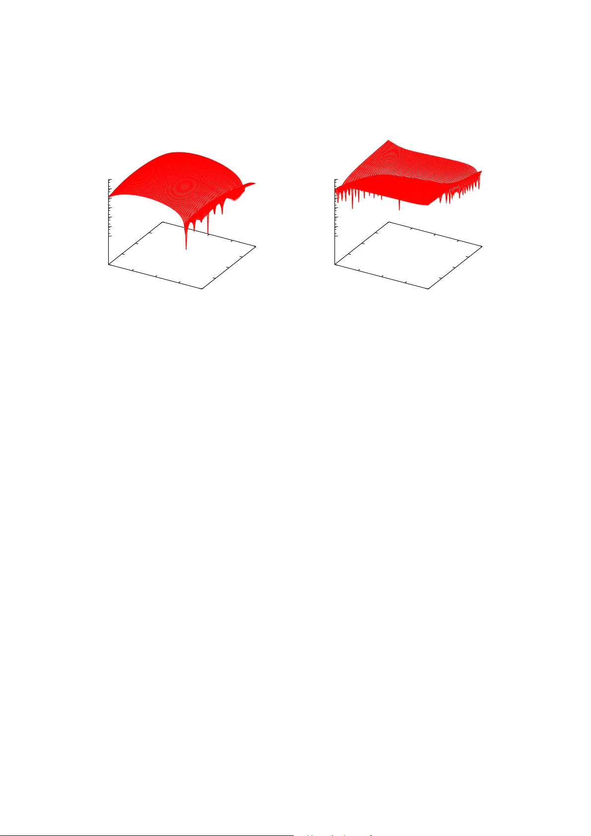
A Dynamic Bi-or thogo nal Field Equat ion Approac h for Efficien t Ba y esian Cali brati o n of Larg e-Scale S y stems ✩ Piyush M. T agade a,1 , Han-Lim Choi a,2, ∗ a Division of A er o sp ac e Engi neering, KAIST, Daeje on 305-701, R e public of Kor e a Abstract This pap er propos es a novel computationally efficient dynamic bi-or thogonality based approa ch for cali- bration of a computer simulator with high dimensional para metric and model str ucture uncertaint y . The prop osed method is based on a deco mp os ition of the solution into mea n and a ra ndom field us ing a generic Karhunnen-Lo eve e xpansion. The random field is repres e n ted as a conv olution of separable Hilber t s pa ces in sto chastic a nd spatial dimensions that are sp ectrally repre s ent ed using respec tiv e orthog onal bases. In particular, the pr esent pa per inv estigates generalize d Polynomial Chaos bas es for sto chastic dimension and eigenfunction bases for spatial dimension. Dyna mic orthogo nality is used to derive closed form equations for the time evolution of mean, spatial and the sto chastic fields. The r esultant system of equations consists of a partial differential equatio n (P DE) that define dynamic evolution of the mea n, a set of PDEs t o define th e time evolution of eigenfunction bases, while a set of ordinary differential equations (ODEs) define dynamics of the sto chastic field. This system of dynamic evolution equations efficiently propag ates the prior para- metric uncertaint y to the system respo nse. The resulting bi-ortho g onal expansion of the system resp o nse is used to reform ulate the Bay esian inference for efficie nt explor ation o f the p oster ior distribution. Efficacy of the propo sed metho d is inv estigated for calibration o f a 2D trans ien t diffusion simulator with unce r tain source lo cation and diffusivity . Computational e fficie ncy of the method is demonstra ted a gainst a Monte Carlo metho d and a ge ne r alized Polynomial Chaos approa ch. Keywor d s: Bay esian F ramework, Dynamically Bi-ortho g onal Field Equations, Kar hun nen-Lo eve Expansion, Ge ner alized Polynomia l Chao s Bas is 1. I n tro duction Recent adv ancements in digita l technologies have facilitated the use o f computer simulators for investi- gation of lar ge scale systems. How ev er, computer s im ulators a re fraught with uncerta inties due to po or ly known/unkno wn mode l, para meters, initial and b ounda ry conditions etc. [ 15 ]. V ar ious rese archers hav e in- vestigated effect of these uncertain ties o n the c r edibilit y of a computer simulator and established uncertaint y quantification and calibratio n a s an in tegral asp ect of a mo deling and simulation pro cess [ 28 , 29 , 32 , 27 ]. This pap er fo cuses o n the Bay esian appr oach that provide a forma l framework to identify , characterize and quantify the uncertainties, and provides a gener ic inference metho d for ca libration of a computer simulator using limited and no isy ex p er imen tal da ta [ 12 , 3 , 1 1 , 13 , 7 ]. The Ba yesian framework is preferre d ov er more traditional calibration metho ds due to its a bilit y to provide complete p oster ior statistics of the par ameters of interest. Sampling techniques s uc h as Markov ✩ This w ork was supported by Basic Science Researc h Program through the National Research F oundation of Korea (NRF) funded by th e Mini stry of Education, Science and T echnology (2010-0025484 ). ∗ Corresp onding Author Email addr esses: piy ush.tagade@ kaist.ac.kr (Piyush M. T aga de), hanlimc@kaist.a c.kr (Han-Lim Choi) 1 Po stdoctoral Research F ello w 2 Assistant Professor Pr eprint submitt ed to Computational Statistics and Data A nalysis Novemb er 7, 2018 Chain Mont e Car lo (MCMC) metho d [ 9 , 2 ] a re used for explor ation of the pos terior statistics, espe cially for calibration of nonlinear dynamical simulators in non-Gauss ian settings. Satisfactory a pproximation o f the po sterior distribution a nd asso cia ted s tatistics using MCMC requires ev aluation of the sim ulator at large nu mber of input settings, o ften in the r ange of 10 3 − 1 0 6 . Collection of la rge num b er o f sa mples bec ome computationally prohibitive for simulation of a large sca le sy stem, imp osing k ey ch allenge for implementation of the Bayesian framework. T o make the Bay esian framework accessible to large-sca le problems, it is necessary to develop co mputationally efficient uncerta in ty propaga tion a nd ca libration techniques. Marzouk et a l. [ 33 ] hav e pr op osed c o mputationally efficient implementation of the Bayesian framework using sto chastic spectra l methods. Stochastic sp ectral pro jection (SSP) based metho ds a re extensively used for uncertaint y pro pagation as a computationally efficient alterna tiv e to Monte Car lo metho ds with comparable accura cy . Homogeneo us Chaos theory in tro duced by Wiener [ 16 , 17 ] is a n ea rliest exp osition of SSP metho d, where r a ndom v ariables a re repr esented as an ex pa nsion ser ies in orthogo nal Hermite po lynomials that conv erges in mean-sq uare sense [ 23 ]. Presen t state of the art in the field of SSP ba sed metho ds for uncertaint y pro pa gation is base d on the gener alized Polynomial Chaos (gPC) metho d. The metho d has be e n succ e s sfully implemented for solution of sto chastic finite element metho ds [ 2 1 , 19 , 22 ] and sto chastic fluid flow pro ble ms [ 18 , 5 ]. Xiu and Ka rniadakis [ 6 ] hav e ex tended the metho d to a set of Askey sc heme of orthog o nal polyno mials. Subsequently , the metho d has b een applied by v arious researchers for uncertaint y pro pagation through simulators of systems o f engineering impo rtance [ 4 , 10 , 30 , 8 ]. The Bay esian ca libration fo rmulation pr op osed by Marzo uk et a l. [ 33 ] us e s the gPC metho d to propag ate the prior par ametric uncertaint y to the s im ulator pre dic tio n. Resultant gPC expa nsion of the predictio n is used in the Bayes theorem to define the likelihoo d. The methodo logy is further extended by Marzouk and Na jm [ 34 ] for inference o f s pa tially/temp orally v arying uncertain parameters . Although the gPC metho d pr ovides computationa lly efficient estimation of the uncerta int y , computa- tional co st of the implementation g rows significantly as the num ber of sto chastic dimensio ns increa ses [ 25 ]. Such a high dimensio nal uncerta int y typically arises for a simulator with a la r ge num ber of uncertain pa- rameters, a nd mo r e predo minantly in the case of a spatially/ tempo rally v arying uncertain pa rameter with rapidly decaying cov aria nce functions. The resea rch work pr esented in this pap er addresse s the B ay esian framework for ca libration of a simulator with high dimensional uncertaint y . Sapsis and Lermusiaux [ 24 ] hav e pr o po sed dyna mica lly orthogo nal field equa tions (DOFE) metho d for efficient propaga tion of high-dimensional uncertaint y . The metho d uses decompositio n o f the s ystem respo ns e int o a mean and sto chastic dynamical comp onent using a tr unca ted genera lized Karhunnen-Loeve expansion. The sto chastic comp onent is sp ectra lly represented in t erms of orthog o nal eigenfunction basis in spatial dimension, while th e respective co efficien ts define the time v a r ying sto chastic dimensio n. The Dyna mic Orthogo nality (DO) co ndition [ 24 ] is use d to derive the clos ed form evolution equations for the mean, eigenfunction ba sis and the s to chastic co efficients. How ev er, the dynamic evolution equations of Sapsis and Lermusiaux [ 24 ] do es not impos e any geometric structure on s to c hastic dimension, w hich ma kes it hard to directly apply the DOFE metho dology for Bay esian calibration pr oblems. This paper propos es a dynamic b i-orthog onality-based a pproach that extends the DOFE metho d for the Bay esian calibration of a computer simulator with high dimensional uncertaint y . The prop osed bi-orthog o nal metho d uses s p ectr a l expansio n of the sto chastic field in the g PC ba s is, impo sing geometric structure on the sto chastic dimension. The rando m coefficients of the trunca ted genera lized Karhunnen-Lo eve expansion, o bta ined using dynamica lly ortho gonal field e q uations, a r e pro jected on the gPC basis using Galerk in pr o jection [ 22 ]. The resultant field equations are termed her e as dynamically bi- orthogo nal field equa tio ns (DBFE). The Bay esian c a libration approach pro po sed in this pap er use s DBFE to pro ject the pr ior pa rametric uncer taint y to the system resp ons e . The resultant bi-o rthogona l expansion is used in the likelihoo d dur ing MCMC sampling for Bayesian infere nce o f the uncertain par ameters. The prop osed DBFE metho d provides substantial computatio nal sp eedup ov er gPC based metho d for Bayesian calibration. Efficacy of the propo sed method is demonstrated for calibration of a 2D transien t diffusion equation simulator with uncertain source lo cation and the diffusivity field. Note that a pr e liminary version of this work was repo rted in [ 26 ], while this a rticle includes (a) extension of the metho d to take in to acc o unt mo del structura l uncertaint y; (b) substantially refined and expanded theo r etical analysis ; and (c) a dditional nu merical r esults demo nstrating computational efficiency of the prop osed metho dolo gy . 2 The res t of the pap er is org anized a s follows. In section 2, statistical formulation is dis cussed in detail. The prop osed DBFE-bas e d Bay esian metho d is presented in section 3 . Section 4 pr ovides numerical results for 2 D transient diffusion equatio n. Finally , the pap er is summariz e d and concluded in section 5 . 2. Statistical F orm ulation The prop os ed Bayesian framework is dev elop ed for a s im ulator T ( x , t, θ ( ω )), where t ∈ R ≥ 0 is time, x ∈ X ⊂ R d is a spa tial dimension and θ ( ω ) is a set o f uncer tain par a meters that induces uncer taint y in the predictions. No te that the simulator T ( x , t, θ ( ω )) is defined over a pro bability space (Ω , F , P ) , wher e ω ∈ Ω is a set of elementary even ts, F is asso c iated σ -algebr a and P is a pr obability measur e defined over F . In this pa per , the pr op osed metho d is particular ly developed for simulators with a mo del g iven by the partial differential equation of type ∂ u ( x , t ; ω ) ∂ t = L [ u ( x , t ; ω ); θ ( ω )] , ( SPDE ) where u ( x , t ; ω ) is the s ystem resp ons e a nd L is an arbitrary differential oper ator. Equation ( SPDE ) is kno wn as stochastic partial differential eq ua tion (SPDE). ( SPDE ) is initialize d using a random field u ( x , 0; ω ), while, the b oundary condition is given by B ( β , t ; ω ) = h ( β , t ; ω ); β ∈ ∂ X , ω ∈ Ω , (1) where B is a linear differential op era tor. The simulator T ( x , t, θ ( ω )) approximates the physical phenomena within the limits of av ailable knowl- edge. Let ζ ( x , t ) b e the ‘true’ but unknown mo del that p erfectly represents the physical phenomena. Since T ( x , t, θ ( ω )) is an a pproximate repr esentation of the physical phenomena, the sim ulator predictions deviates from ζ ( x , t ) by δ ( x , t ), wher e δ ( x , t ) is known as the discr epancy function. The r elationship b et ween ζ ( x , t ) and T ( x , t, θ ( ω )) is given by [ 12 ] ζ ( x , t ) = T ( x , t, ˆ θ ( ω )) + δ ( x , t ) , (2) where ˆ θ ( ω ) denotes the ‘true’ v alue of the uncertain para meter s. The prop osed Ba yesian framework uses ex per imen tal observ ations at finite lo cations for inference of the uncer tain par a meters. At time t , let the system b e experimentally observed at M spa tial lo cations { x i ; i = 1 , . . . , M } . The measur e men t at x i , denoted a s y e ( x i , t ), is given by y e ( x i , t ) = ζ ( x i , t ) + ǫ ( x i , t ) , (3) where ǫ ( x i , t ) is the measurement uncertaint y . Let y e = { y e ( x i , t ); i = 1 , ..., M } b e the set of av ailable exp erimental o bserv ations. Using y e , the uncertain parameter s θ a nd the discrepancy function δ ( x , t ) ca n be inferred through the Bay es theo rem as f  ˆ θ ( ω ) , δ ( x , t ) | y e  ∝ f  y e | T ( x , t, ˆ θ ( ω )) , δ ( x , t )  × f  ˆ θ ( ω ) , δ ( x , t )  , (4) where f ( ˆ θ ( ω ) , δ ( x , t )) is the pr ior, f ( y e | T ( x , t, ˆ θ ( ω )) , δ ( x , t )) is the likelihoo d and f ( ˆ θ ( ω ) , δ ( x , t ) | y e ) is the p os terior pro bability distribution. Uncertaint y in the exp er imental observ ations, ǫ ( x , t ), is assumed to be specified using a zer o mean Gaussian distributio n with cov ariance matrix Σ e = σ 2 e I M , (5) where I is the M × M identit y matrix . In this pa p er , the pro po sed Bayesian framework is develope d for independent pr ior uncerta int y in ˆ θ ( ω ) and δ ( x , t ), with the prior for δ ( x , t ) given by a zero - mean Gaussian pro cess with a cov a riance function of the form Σ δ ( x 1 , x 2 ) = σ 2 δ exp − d X i =1 λ i  x i 1 − x i 2  2 ! , (6) 3 where σ 2 δ is the v ariance and λ i is the correla tion strength of the cov ariance function, w hich ar e treated as uncertain h yper -parameters . In the pr esent pap er, inv erse Gamma prior I G ( α σ , β σ ) is used for σ 2 δ , while, the Gamma pr ior G ( α λ i , β λ i ) is used for λ i [ 12 , 20 , 1 ]. The uncertaint y in δ ( x , t ) is s pecified us ing hiera rchical zero-mea n Gaussia n pro ces s prio r as f ( δ ( x , t ) , σ 2 δ , λ i ) ∝| Σ δ | − 1 2 exp  − 1 2 δ T Σ − 1 δ δ  × ( σ 2 δ ) − α σ − 1 exp  − β σ σ 2 δ  × d Y i =1 ( λ i ) α λ i − 1 exp ( − β λ i λ i ) (7) where δ = { δ ( x i , t ); i = 1 , ..., N } . Use ( 7 ) and ( 5 ) in the Bay es theorem ( 4 ) and marginalize δ ( x , t ) to obtain f ( ˆ θ ( ω ) , σ 2 δ , λ i ) ∝| Σ | − 1 2 exp  − 1 2 η T Σ − 1 η  × ( σ 2 δ ) − α σ − 1 exp  − β σ σ 2 δ  × d Y i =1 ( λ i ) α λ i − 1 exp ( − β λ i λ i ) × f ( ˆ θ ( ω )) , (8) where Σ = Σ δ + Σ e and η = { y e ( x i , t ) − T ( x i , t, ˆ θ ( ω )); i = 1 , ..., M } . 3. Prop osed Metho dology Equation ( 8 ) can b e solved by sampling fr om the po sterior distribution using MCMC, which requires ev aluation of T ( x i , t, ˆ θ ( ω )) for each sample, which is computationally prohibitiv e for large-scale system simulators. The approa ch pro po sed in this pap er requires single ev aluation of ( SPDE ) using dynamica lly bi-orthogo nal field equations. The DBFE is used for propagating the pr ior uncertaint y in ˆ θ ( ω ) to the system resp onse. The resulta n t bi-orthog o nal expansion of the s ystem resp onse is us e d in ( 8 ) to define the p osterio r distribution, which is explored using the MCMC. The prop osed metho d is describ ed in detail in this section. 3.1. Dynamic al ly Bi-ortho go nal Field Equations The pro p os ed DBFE metho d is bas ed o n the dynamica lly orthogo nal field equa tions (DOE F) prop osed by Sapsis and Lermusiaux [ 24 ]. Co nsider a generic Kar hunnen-Lo eve expansio n of u ( x , t ; ω ) truncated at N terms as u ( x , t ; ω ) = u ( x , t ) + N X i =1 Y i ( t ; ω ) u i ( x , t ) , (9) where u ( x , t ) is the mea n, u i ( x , t ) are the functions that form the complete o r thonormal bas is on L 2 ( X ), while Y i ( t ; ω ) are the zero-mean independent random v ar iables. Note that thr oughout this paper the equa lity sign, =, is used to represent the approximate equalit y , if no confusion is expected. Substituting the expansion ( 9 ) in ( SPDE ) g ives ∂ u ( x , t ) ∂ t + N X i =1 u i ( x , t ) d Y i ( t ; ω ) dt + N X i =1 Y i ( t ; ω ) ∂ u i ( x , t ) ∂ t = L [ u ( x , t ; ω ); θ ( ω )] . (10) Note that the quan tities u ( x , t ), Y i ( t ; ω ) and u i ( x , t ) are dep endant on each other through ( 9 ). Thus, v arying u ( x , t ), Y i ( t ; ω ) and u i ( x , t ) concurr ent ly ma kes ( 10 ) r edundant, necessita ting imp osition of the additiona l constraint to de r ive the indep endent evolution equations for unknown quantities. Sapsis and Ler m usiaux [ 24 ] prop ose d impo sition of dynamic orthog o nality (DO) condition to derive the independent evolution equa tions for u ( x , t ), Y i ( t ; ω ) and u i ( x , t ). The DO condition constraints the time evolution o f u i ( x , t ) such that  ∂ u i ( x , t ) ∂ t , u j ( x , t )  X = 0; ∀ i, j = 1 , ..., N , (11) where h· , ·i is inner pro duct. Note that the DO co ndition ensures that u i ( x , t ) pres erves o rthonormality o ver the time evolution of ( SPDE ). 4 Remark 1. In this p ap er, inner pr o duct is define d over sp atial and sto chastic dimensions. Inner pr o duct over the sp atial dimension is define d as h u ( x , t ; ω ) , v ( x , t ; ω ) i X = Z X u ( x , t ; ω ) v ( x , t ; ω ) d x , (12) while t he inner pr o duct over t he sto chastic dimension is define d as h u ( x , t ; ω ) , v ( x , t ; ω ) i Ω = Z Ω u ( x , t ; ω ) v ( x , t ; ω ) d P ( ω ) . (13) Using the DO co ndition, the indep endent ev olution equations for u ( x , t ), u i ( x , t ) and Y i ( t ; ω ) ar e der ived as fo llows [ 24 ]. 3.1.1. Dynamic al ly Ortho gonal Field Equations Apply the e x pecta tion op erator to ( 10 ) to o bta in the evolution equatio ns for u ( x , t ) as ∂ u ( x , t ) ∂ t = E ω [ L [ u ( x , t ; ω ); θ ( ω )]] . (14) Multiply ( 10 ) by Y j ( t ; ω ) and apply the exp ectation op era tor to hav e N X i =1 C Y i ( t ) Y j ( t ) ∂ u i ( x , t ) ∂ t + N X i =1 C d Y i ( t ; ω ) dt Y j ( t ; ω ) u i ( x , t ) = E ω [ L [ u ( x, t ; ω ); θ ( ω )] Y j ( t ; ω )] , (15) where C Y i ( t ) Y j ( t ) denote the cov ariance betw een Y i ( t ; ω ) a nd Y j ( t ; ω ). By m ultiplying u k ( x , t ) to ( 15 ), taking the inner pr o duct and applying the exp ectation op erator gives C d Y k ( t ) dt Y j ( t ) = h E ω [ L ( u ( x, t ; ω ); ω ) Y j ( t ; ω )] , u k ( x, t ) i X , (16) which o n substitution in ( 15 ) provides N X i =1 C Y i ( t ) Y j ( t ) ∂ u i ( x , t ) ∂ t = E ω [ L [ u ( x , t, ω ); θ ( ω )] Y j ( t ; ω )] − N X k =1 h E ω [ L [ u ( x , t, ω ); θ ( ω )] Y j ( t ; ω )] , u k ( x , t ) i X u k ( x , t ) . (17) Equation ( 17 ) can b e written in the matrix form U = Γ − 1 D , (18) where Γ is the cov a riance matrix with ( i, j ) th element Σ ij = C Y i ( t ) Y j ( t ) . T o der ive the evolution equa tion for Y j ( t ; ω ), mult iply b oth sides of ( 10 ) by u j ( x , t ) a nd take the inner pro duct to o btain  ∂ u ( x , t ) ∂ t , u j ( x , t )  X + N X i =1 h u i ( x , t ) , u j ( x , t ) i X d Y i ( t ; ω ) dt + N X i =1 Y i ( t ; ω )  ∂ u i ( x , t ) ∂ t , u j ( x , t )  X = hL [ u ( x , t ; ω ); θ ( ω )] , u j ( x , t ) i X . (19) Note that the third term of left hand side in ( 19 ) v anishes completely due to the DO condition ( 11 ), while, the s econd ter m v anishes for all i 6 = j owing to the orthonor mality of u i ( x , t ), thus d Y i ( t ; ω ) dt +  ∂ u ( x , t ) ∂ t , u i ( x , t )  X = hL [ u ( x , t ; ω ); θ ( ω )] , u i ( x , t ) i X . (20) 5 Note that multiplying ( 14 ) by u i ( x , t ) a nd ta king inner pro duct g ives  ∂ u ( x , t ) ∂ t , u i ( x , t )  X = h E ω [ L [ u ( x , t ; ω ); θ ( ω )]] , u i ( x , t ) i X . (21) Using ( 21 ) in ( 2 0 ) gives the evolution eq uation for Y i ( t ; ω ) as d Y i ( t ; ω ) dt = hL [ u ( x , t ; ω ); θ ( ω )] − E ω [ L [ u ( x , t ; ω ); θ ( ω )]] , u i ( x , t ) i X . (22) 3.1.2. Bi-ortho go nal Exp ansion Note that the numerical so lution of ( SPDE ) using the DOFE metho d pr ovide the samples of u ( x , t ; ω ) through the co efficie n ts Y i ( t ; ω ), whereas, the Bayesian inference r equires analy tic for m o f the pro ba bilit y distribution of the system respons e , th us, the DOFE method can not directly b e used f or the Bay esian inference. In the present paper, a bi-orthogo nal ex pansion approach is prop os ed to impos e the orthogo nality based g eometric structure on the sto chastic dimension. Consider a gPC expansio n of Y i ( t ; ω ) trunca ted at P terms as Y i ( t ; ω ) = P X p =1 Y i p ( t ) ψ p ( ξ ( ω )) , (23) where ψ p ( ξ ( ω )) are the o r thogonal p olynomials from the Askey sc heme, while ξ ( ω ) ∈ L 2 (Ξ) a re the random v ariables with appropria te probability densit y function [ 6 ]. Use ( 23 ) in ( 9 ) to g et u ( x , t ; ω ) = u ( x , t ) + N X i =1 P X p =1 Y i p ( t ) ψ p ( ξ ( ω )) u i ( x , t ) . (24) Equation ( 24 ) is termed her e as the b i-orthog o nal expa nsion. Differentiate ( 2 3 ) with r esp ect to time a nd use the Galer kin pro jection to o bta in d Y i p ( t ) dt = 1  ψ 2 q  Ω D h F [ u ( x , t ; ω ); θ ( ω )] − E ω [ F [ u ( x, t ; ω ); θ ( ω )]] , u i ( x , t ) i X , ψ p ( ξ ( ω )) E Ω . (25) Equations ( 14 ), ( 17 ) and ( 25 ) fo r ms dynamically bi-o rthogonal field equations (DBFE) that define the dynamic evolution of the mean u ( x , t ), the eigenfield u i ( x , t ) a nd the asso cia ted co e fficien ts Y i p ( t ). The resultant bi-orthogonal expansion ( 24 ) approximates the system resp onse u ( x , t ; ω ) to a n arbitra ry accuracy depe nding on the num b er of eig enfunctions used, N , and the n um ber of expansion co efficients for each eigenfunction, P . 3.1.3. Boundary Conditions T o define b oundar y co nditions for DBFE, co ns ider a gener ic Karhunnen-Lo eve expansion of h ( β , t ; ω ) h ( β , t ; ω ) = h ( β , t ) + N X i =1 Y i ( t ; ω ) u i ( β , t ) . (26) Applying the exp ectation o pe rator to ( 26 ), b ounda ry co ndition for the mea n is given by B ( u ( x , t )) = h ( β , t ) . (27) By multip lying Y j ( t ; ω ) t o ( 26 ) a nd applying the expectation o pe rator to obtain boundary co nditio n for u i ( x , t ) B ( u i ( β , t )) = N X j =1 C − 1 Y i ( t ) Y j ( t ) E ω [ h ( β , t ; ω ) Y j ( t ; ω )] . (28) 6 3.2. Bayesian In fer enc e Without los s of genera lit y , the pro po sed metho d is des crib ed here for a spatially v a r ying uncertain parameter with prior given by a scalar s to chastic pro cess v ( x ; ω ), i.e. θ ( ω ) = { v ( x ; ω ) } . Us e a KL expansion o f v ( x ; ω ) as v ( x ; ω ) = v ( x ) + N X i =1 p λ i v i ( x ) χ i , (29) where χ i are independent identically distributed zero-mea n r andom v ariables, while, λ i and v i ( x ) a re the eigenv alues and eig e nfunctions of the c ov ariance function of v ( x ; ω ). F o r the cov ariance function C v ( x 1 , x 2 ), λ i and v i ( x ) a re solution of the eigenv a lue pro blem Z X C v ( x 1 , x 2 ) ν i ( x 1 ) d x 1 = λ i v i ( x 2 ) . (30) F or a Gaussian pro cess prior, χ i are standar d norma l r andom v ariables, whereas, for a g eneric sto chastic pro cess prio r, χ i are given by χ i = 1 √ λ i Z X ( v ( x ; ω ) − v ( x )) v i ( x ) d x . (31) Use the gPC expa nsion o f χ i χ i = P X p =1 ˆ χ i p ψ p ( ξ ( ω )) , (32) where ˆ χ i p are the gP C expans ion co efficients, in ( 29 ) to get the bi-o rthogona l expa nsion of v ( x ; ω ) as v ( x ; ω ) = v ( x ) + N X i =1 P X p =1 p λ i v i ( x ) ˆ χ i p ψ p ( ξ ( ω )) . (33) The expansion ( 33 ) is used in L [ u ( x , t ; ω ); θ ( ω )] to define the RHS of the DBFE gov erning equations (( 14 ), ( 17 ) and ( 2 5 )). The numerical solution o f the res ultant DBFE gov erning equations give the bi-or thogonal expansion ( 24 ) of the system resp onse u ( x , t ; ω ). Remark 2. The numeric al solution is initiate d with the initial c ondition for the me an u ( x , t ) given by u ( x , t ) = E ω [ F [ u ( x , 0; ω ); θ ( ω )]] , (3 4 ) while, the initial c onditions for the eigenfield ar e given by u i ( x , t ) = v i ( x ) . (35) Sinc e the st o ch asticity in ( SPDE ) emanates due to the unc ertainty in ν ( x ; ω ) , ( SPDE ) is initialize d with a deterministic initial c ondition. Thus, the initial c ondition for the exp ansion c o effici ents Y i p ( t ) is given by Y i p (0) = 0; ∀ i = 1 , .., N ; p = 1 , ..., P. (36) The bi-orthog onal expansion of u ( x , t ; ω ) is used in ( 8 ) to define the likeliho o d f ( y e | ξ , σ 2 δ , λ i ) ∝| Σ | − 1 2 exp  − 1 2 η T Σ − 1 η  , (37) where η = ( y e ( x k , t ) − u ( x k , t ) + N X i =1 P X p =1 Y i p ( t ) u i ( x k , t ) ψ p ( ξ ( ω )) ! ; k = 1 , ..., M ) . (38) 7 Note that co nditional on the hyper-par a meters of the discre pa ncy function, σ 2 δ and λ i , ξ a re the o nly uncertain pa rameters in ( 37 ). Thus, the Bayesian ca libr ation problem is r e formulated in the space L 2 (Ξ) as the inference of ξ . In the pr e sent pap er, the pr op o sed metho d is demons trated for Hermite p olyno mials as g PC basis, wher e ξ ar e the indep endent identically distributed s ta ndard no rmal r andom v ariables, th us, the pr ior for ξ is given by f ( ξ ) ∝ N z Y k =1 exp  − ξ 2 k 2  , (39) where N z is the dimens io n of s tochasticity . Using ( 39 ) a nd ( 37 ) in ( 8 ), the pro po sed fo rmulation for the Bay esian inference is f ( ξ , σ 2 δ , λ i ) ∝| Σ | − 1 2 exp  − 1 2 η T Σ − 1 η  × ( σ 2 δ ) − α σ − 1 exp  − β σ σ 2 δ  × d Y i =1 ( λ i ) α λ i − 1 exp ( − β λ i λ i ) × N z Y k =1 exp  − ξ 2 k 2  . (40) Note that ( 40 ) do e s not inv olve the solution of T ( x , t, θ ( ω )), thus, the p oster ior distribution can can b e explored efficiently using MCMC. In the present pap er, Metro po lis-Hastings algor ithm [ 14 , 31 ] is used to sample fr o m the p osterio r distribution. 4. Numerical Example: 2D T ransien t Diff usion Equation The efficacy and efficiency o f the prop osed metho d is inv estigated for calibra tion of a tw o-dimensional transient diffusion simulator with uncer tain sour ce lo cation and diffusivit y field. Presen t pap er co nsiders a sto chastic tra nsient diffusion equa tio n defined ov er a tw o-dimensiona l do main X = [ − 1 , 1] × [ − 1 , 1] with adiabatic b oundar y conditions as ∂ u ( x , t ; ω ) ∂ t = ∇ ( ν ( x ; ω ) ∇ u ( x , t ; ω )) + N s X l =1 s l 2 π σ 2 exp − ( z l − x ) 2 2 σ 2 l ! (41) ∇ u ( x , t ; ω ) · ˆ n = 0 (42) u ( x , t ; ω ) = 0 , (43) where ν ( x ; ω ) is spatially v ar ying diffusivity field, while tota l N s source term are activ e a t lo ca tions z l with s ource strength S l . The diffusivity field, ν ( x ; ω ), and the lo cation of the sour ce, z , ar e ass umed to be uncertain. Efficacy of the pro po sed metho d is demonstrated using the ‘hypothetica l test b ed’ da ta , which is defined us ing the numerical solution of ( 43 ) for co mpletely k nown source lo cation and the diffusivity field. In the pres e nt pap er , the pro p os ed metho d is demonstra ted for a single so urce lo cated at (0 . 2 , − 0 . 2), which is ac tive during time [0 , 0 . 01]. The spatia l v ariation of the diffusivity is assumed to take the form ν ( x ) = 0 . 05( ν 0 + 10 . 0 + 0 . 25 x + 0 . 65 y + x 3 + y 3 ) , (44) where ν 0 is a user defined constant. Figure 1 (a) shows spatial v ariation of the diffusivit y . The deterministic nu merical solution is o bta ined using a second or der central difference scheme in spa tial dimensio n with uni- form grid spacing h = 0 . 02, while the explicit fourth or der Runge- Kutta s cheme is used for time integration with the time step ∆ t = 0 . 0 001. Fig ure 1 (b) s hows the numerical s olution at t = 0 . 05 s , while the so lution at t = 0 . 1 s is shown in Fig ure 1 (c). Note that the source has p eak streng th at z l and reduces ex po nen tially with the dis ta nce, res ulting in the p ea k v alue of u a t the sour c e lo catio n and the subsequent diffusion with time to other lo cations . Up on re mov al o f the source, diffusion of u is no n-uniform owing to the non-linear diffusivit y . 8 -1 -0.5 0 0.5 1 -1 -0.5 0 0.5 1 0 1 2 v Diffusivity x y v (a) s patial v ariation of diffusivit y -1 -0.5 0 0.5 1 -1 -0.5 0 0.5 1 0 2 4 6 8 u time=0.05s x y u (b) u-field at t = 0 . 05 s -1 -0.5 0 0.5 1 -1 -0.5 0 0.5 1 0 2 4 6 8 u time=0.1s x y u (c) u- field at t = 0 . 1 s Figure 1: Solution of tw o-dimensional transient diffusion equation 4.1. DBFE F ormulation F or no tational conv enience, define S ( x ; ω ) = s 2 π σ 2 exp − ( z − x ) 2 2 σ 2 ! , (45) which is uncertain owing to the unce r taint y in the sour ce loca tion z . The prior uncertaint y in z is expanded in a g PC basis, while the Galerkin pro jection is used to obtain the r esultant g PC co efficien ts, ˆ S ( x ), o f S ( x ; ω ) = P X p =1 ˆ S ( x ) ψ p ( ω ) . (46) The pr ior uncer taint y in ν ( x ; ω ) is represented using a Ga us sian pro cess, whic h is spe ctrally r epresented using the bi-o rthogona l expa nsion a s ν ( x ; ω ) = ν ( x ; ω ) + N X i =1 P X p =1 V i p ν i ( x ) ψ p ( ω ) , (47) where ν ( x ; ω ) is the mean, ν i ( x ) are the eigenfunctions of the c ov ariance function of ν ( x ; ω ) and V i p are the resp ective expansion co efficients. Use ( 46 ) and ( 4 7 ) in ( 43 ) to o btain the differential op erator in ( SPDE ) as L [ u ( x , t ; ω ); θ ( ω )] = ∇ [ ν ( x ) ∇ u ( x , t ) + ν ( x ) N X i =1 P X p =1 Y i p ( t ) ψ p ( ξ ( ω )) ∇ u i ( x , t ) + N X i =1 N X j =1 P X p =1 P X q =1 V i p Y j q ( t ) ν i ( x ) ψ p ( ξ ( ω )) ψ q ( ξ ( ω )) ∇ u j ( x , t ) + N X i =1 P X p =1 V i p ν i ( x ) ψ p ( ξ ( ω )) ∇ u ( x , t )] + P X p =1 ˆ S ( x ) ψ p ( ξ ( ω )) . (48) Use ( 48 ) in ( 1 4 ), ( 17 ) a nd ( 25 ) to obtain the DBFE gov erning equa tio ns for the t wo-dimensional transient- diffusion equa tio n. 9 10 -1 10 0 10 1 10 2 10 3 10 4 10 5 1 2 3 4 5 6 7 Time, s No. of eigenfunctions, N MC dbfe, p=1 dbfe, p=2 dbfe, p=3 gpc, p=1 gpc, p=2 gpc, p=3 (a) C P U tim e 0.01 0.1 1 1 2 3 4 5 6 7 Error No. of eigenfunctions, N dbfe, p=1 dbfe, p=2 dbfe, p=3 gpc, p=1 gpc, p=2 gpc, p=3 (b) L 1 -error Figure 2: Compari son of accuracy and computational efficiency of DBFE with gPC and Monte Carlo method 4.2. Solution of F orwa r d Pr oblem The prior uncertaint y in the s o urce lo cation is sp ecified using indep endent Gaus sian distribution fo r x and y co -ordinate with mean 0 a nd standard deviation 0 . 3 , while, the prior for diffusivity ν ( x ; ω ) is sp ecified using a Gauss ian pro c e ss with mean ν ( x ) = 0 . 05( ν 0 + 10 . 0 + 0 . 25 x + 0 . 65 y ) (49) and the squa red exp onential cov ariance function C ( x 1 , x 2 ) = σ 2 ν exp  − λ 1 ( x 1 − x 2 ) 2 − λ 2 ( y 1 − y 2 ) 2  , (50) where σ 2 ν is the v ariance of the Gaus sian pr o cess a nd λ i is the cor relation leng th. Efficacy and the computatio nal efficiency o f the pro p os ed B ay esian inference dep ends o n the ability of the DBFE method to accura tely so lve the forward forward pr oblem. In the presen t subsection, accuracy and the computational co st for the numerical implementation of DBFE is compar ed a gainst the Monte Carlo and the ge ner alized Polynomial Chao s metho d (see [ 33 ] for the g PC for m ulation of ( 4 3 )). Figure 2 shows the accura c y and computational efficiency of the DBFE and the gPC metho d for different v alues of num b e r of eigenfunctions used, N , and the or der of the p olynomia l chaos basis, p . The accurac y is compared using the Monte Carlo metho d with 1000 0 s amples, whic h ar e collected at the computational cost of 6616.1 7 s econds. The computational co st for solution of the forward problem increases with incre ase in N and p for b oth the DBFE and g PC metho d. Note that the sto chastic dimensio n for the present pro blem is N + 2 ( N dimensio ns represe nting the truncated KL expansion, while 2 dimensions r epresenting unce r taint y in the sour ce lo catio n), for which the num ber of p olynomia l chaos terms is g iven by P = ( N + 2 + p )! ( N + 2)! p ! + 1 . (51) Since implemen tation o f the gPC metho d requir es n umerical solution of P PDEs (see [ 34 ] for details), whereas, the DBFE metho d inv olv es numerical solution of ( N + 1 ) PDEs and N × P ODEs, the incr ease in computational cost with p is significa nt ly higher for the gP C metho d as compar ed with the DBFE metho d. The c omputational cost of the gPC metho d is comparable t o the Mon te Ca rlo metho d for N = 6 a nd 10 second order p olynomial chaos basis , while the computational cost is higher than the Monte Car lo metho d for third order p olynomia l chaos basis with N ≥ 3, render ing the g PC metho d computationa lly intractable. The DBFE metho d is numerically implemented at a computational cost comparable to the g PC metho d for p = 1 , while, the co mputational cost fo r the DBFE metho d for p ≥ 2 is consider a bly low er than the gPC metho d. The L 1 -error in v ariance is shown in Figure 2 (b). The err or is compa rable for b oth the DBFE and the gPC metho d, which decrease with N and rea ches the limiting v alue for N ≥ 4 , though the limiting v alue is higher for p = 1. Note that the trans ie n t diffusion equatio n inv olves multiplication of the diffusivity ν with ∇ u , thus, a ppropriate sp ectral representation r equires use of the seco nd order p olynomial chaos bas is . F rom the results, it may b e concluded that ( 43 ) can be numerically solved using the DBFE meth o d at significantly lower co mputational c o st than the gP C metho d with the compar able accura cy . 4.3. Solution of Sou rc e Inversion Pr oble m The prop osed metho d is used for inference of the s o urce lo c a tion and the diffusivity . Prior uncer taint y in the so urce lo ca tion is given by indep endent Gaussian pro ce s ses in x a nd y directions , with N (0 . 0 , 0 . 3) prior. Prio r uncertaint y in the diffusivity is sp ecified using the Ga ussian pr o cess with the mea n ( 49 ) a nd the cov ar iance function ( 50 ) with σ 2 = 0 . 3 and λ = 1 . 5 . The pr ior uncertaint y is propa gated to the system resp onse using t he DBFE metho d with N = 5 and p = 2. The deterministic solution o f the 2D transient diffusion equation at time t = 0 . 02 seconds with the so urce remov ed at t = 0 . 01 seconds is us e d as exp erimental o bserv ations. The sour c e is ass umed to b e lo cated at [0 . 2 , − 0 . 2]. T otal 2 5 uniformly spaced data p oints are used for the Bay esian inference. 1% exp er imen tal uncertaint y is ass umed in each da ta p oint. The mo del s tructure uncer ta in ty is defined by s pecifying the prior pro bability distribution for σ 2 δ and λ δ . Inv erse Gamma distribution I G (6 . 0 , 2 . 0 ) is used for σ 2 δ , while, the prior for λ δ is giv en b y the Gamma distribution G (6 . 0 , 2 . 0). Posterior dis tribution is explor ed by collected 100 00 s amples using MCMC, after burnout p erio d o f 100 0 samples. Figure 3 shows the p os ter ior pro bability density co ntours for the sour c e lo cation. The contour is shown for the p osterior density obtained using the pr op osed metho d (dashed line) and the direct MCMC sampling from the p os ter ior distribution (solid lines). The source lo ca tion is predicted a ccurately , while, the p osterior density obtained using the pr op osed metho d agree s closely with the direct MCMC sampling, demonstrating the e fficacy of the DBFE base d Bay esian inference. Figure 4 (a) sho ws the L 1 -error in p osterio r v ariance of the diffusivit y b etw een the DBFE the dire c t MCMC sampling. The ma ximu m er ror is o f the or der of 1 0 − 3 , indica ting the c lo se agre e men t in v ariance for the p osterior pr obability o f the diffusivit y o btained us ing the DBFE a nd the direct MCMC sampling metho ds. Figure 4 (b) shows the L 1 -error for pos terior mea n of the diffusivity for the DBFE method obtained against the ‘true’ diffusivity . Note that the error reduces non- uniformly , indicating the effect of the lo ca tion of the exp erimental obse r v ations o n the prop os ed Bayesian inference. Figure 5 shows the c o mparison of the p osterio r probability distr ibution of σ 2 δ and λ δ obtained using the direct MCMC sampling and the pro po sed metho d. The po sterior distribution for λ δ obtained using the prop osed metho d ma tc hes clo sely with the direct sampling, how ever, the match is compar atively p o or for the p os terior distribution of σ 2 δ . No te that the bi-ortho g onal expansio n obtained using the DBFE metho d acts as an emulator of the 2D transient diffusio n equation, which is used in the Bayesian inference a s against the simulator in the direct MCMC sampling. Thus, any remnant error in the bi- o rthogona l expansio n is considered as the uncer taint y in the mo del structure, r esulting in the differ ence in the p oster io r probability distribution for σ 2 δ . The posterio r probabilit y fo r λ δ has mo ved tow ards the left for b oth the cases, indicating increased correlation for the mo del structure uncertaint y , while, the posterio r distribution for σ 2 δ mov es tow ards right, indicating higher p osterior confidence on the simulator. Figure 6 shows the L 1 -error in the p osterior mean for the system resp onse u , which is defined aga inst the true spa tia l distribution of u . The p osterior mean o f the system resp onse is calculated by s ubstituting the mean o f ξ in the bi-orthog onal expansio n. The maximum L 1 -error is of the or der o f 10 − 1 , which is lo ca ted in the b oundar y region where exp erimental data is not provided for the Bay esian inference. In the r e gion where e x per iment al observ ations are av a ilable, the er ror is significa ntly low with the minimum v alue of the order o f 10 − 7 . 11 direct dbfe 0.05 0.1 0.15 0.2 0.25 0.3 0.35 x -0.35 -0.3 -0.25 -0.2 -0.15 -0.1 -0.05 y Figure 3: Posterior Probability Con tours for the Source Lo cation 5. Concluding R emarks The pap er has presented a dynamic bi-o rthogona lity based a ppr oach for co mputationally efficient im- plement ation of the Bay esian inference. Th e prop osed metho d can b e a pplied for ca libration of a simulator represented using partia l differential equatio n with high dimensio nal uncerta in ty . Though the metho d re - quires reformulation o f the gov erning equations, existing schemes can be extended in a stra ightf orward manner fo r numerical solution o f the DBFE. Efficacy of the prop osed metho d is demonstrated for calibratio n of a tw o-dimensional tra nsient diffusion equation with uncertain source lo ca tion and the diffusivity . Computational cost of the pr op osed metho d for uncertain ty propaga tion is compared against the gP C a nd the Monte Ca rlo method. Note that for low dimensional uncertaint y , co mputational cost of the g P C metho d is compara ble to the DBFE, howev er, as dimensionality of the uncertaint y inc r eases, the DBFE method provide the solution of the SPDE at a significantly less computational co st than the gPC method with co mparable accuracy . Accura cy of the prop osed metho d to infer the uncerta in pa rameters is compar ed aga inst the direct MCMC sampling. The metho d provide a ccurate inference of the source lo cation with the marginal p osterio r dis tribution matching closely w ith the MCMC sampling. The metho d is found to accur ately infer the p osterio r distribution o f the spatially/temp ora lly v arying par ameters. In the present paper , the pro p os ed method is demonstrated in the Gaussian context. In the future, efficacy of the prop osed metho d will b e demonstrated for a mo r e gener ic non-Gaussian non-stationar y setting. References [1] OHagan A. Bay esian Analysis of Computer Co de Outputs: A Tutorial . R eliability Engine ering and Sy stem Safet y , 91:1290–130 0, 2006. [2] Gamerman D. and Lopes H.F. Markov Chain Monte Carlo: Sto chastic Simulation for Bayesian Infer enc e . Chapman and Hall/CRC, Boca Raton, 2006. [3] Higdon D., Kennedy M., Cav endish J.C., Cafeo J.A., and Ryne R.D. Combining Field Data and Computer Simulations for Calibration and Prediction. SIAM Journal of Scientific Computing , 26(2):448 –446, 2005. 12 -1 -0.5 0 0.5 1 -1 -0.5 0 0.5 1 10 -9 10 -8 10 -7 10 -6 10 -5 10 -4 10 -3 Error x y Error (a) L 1 -error in P osterior V ariance f or DBFE and Direct MCMC Sampling -1 -0.5 0 0.5 1 -1 -0.5 0 0.5 1 10 -7 10 -6 10 -5 10 -4 10 -3 10 -2 10 -1 Error x y Error (b) L 1 -error in Posterior Mean for DBFE Figure 4: L 1 -error in posterior v ariance and mean for diffusivity [4] Lucor D., Xiu D., Su C.H., and Karniadakis G.E. Predictability and Uncertain ty in CFD. International Journal for Numeric al Metho ds in Fluids , 43:483–505, 2003. [5] Xiu D. and Kar niadakis E. The Weiner-Askey Polynomial Chaos for Stochastic Different ial Equations. SIAM Journal of Scientific Computing , 24:619–644, 2002. [6] Xiu D. and Karniadakis G. E . Modeling U ncertaint y in Flow Simulation s via Generalized Polynomial Chaos. Journal of Computational Physics , 187:137–167, 2003. [7] Kelly D.L. and Smi th C.L. Bay esian Inference in Probabilistic Risk Assessm ent - The Cur ren t State of the Art. R eliability Engine ering and Sy stem Safet y , pages 628–643, 2009. [8] P o ette G., Despres B., and Lucor D. Uncertaint y Q uan tification for Systems of Conserv ation Laws. Journal of Compu- tational Physics , pages 2443–2467, 2009. [9] Besag J., Green P .J., Higdon D., and Mengersen K. Bay esian Computation and Sto c hastic Systems. Stati st ic al Scienc e , 10:3–41, 1995. [10] M athelin L., Hussaini M.Y., Zang T.A., and Bataille F. Uncertain ty Pr opagation f or a Tur bulen t, Compressi ble Nozzle Flow usi ng Stochast ic Metho ds. AIAA Journal , 42:1669–1676, 2004. [11] Goldstein M. and Rougier J. Probabilistic Form ulations for Transferring Inferences from Mathematical Models to Physica l Systems. SIAM Journal of Scientific Computing , 26(2):467–487, 2005. [12] K ennedy M.C. and O’Hagan A. Bay esian Cali bration of Comput er Mo dels. Journal of the Ro yal Statistic al So ciety. Serie s B (Statistic al Metho dolo gy ) , 63(3):425–4 64, 2001. [13] B ay arri M.J., Berger J.O., P aulo R., Sacks J., Cafeo J.A., Cav endish J. , Lin C.H., an d T u J. A Framew ork for Validation of Computer Mo dels. T e chno metrics , 49(2):138 –153, 2007. [14] M etropolis N., Rosenbluth A.W., Rosenbluth M.N ., T eller A. H., and T eller E. Equation of State Calculations by Fast Computing Mac hines. The Journal of Chemic al Physics , 21(6):108 7–1092, 1953. [15] O resk es N., Shrader-F rec hett K., and B el i tz K. V eri fication, Vali dation and Confirmation of Numerical Mo dels in Earth Sciences. Science , 26 3(5147):641– 647, 1994. [16] Wiener N. The Homogeneous Chaos. Americ an Journal of Mathematics , 60:897–936, 1938. [17] Wiener N. Nonline ar Pr oblems in R andom The ory . John Wiley & Sons, New Y ork, 1958. [18] K nio O.M . and Maitre O.P . Uncertain t y Propagation in CFD using Polynomial Chaos Decomposition. Fluid Dynamics R ese a r ch , 38:616–640, 2006. [19] Ghanem R. and Red-Horse J. Propagation of Probabilis tic Uncertain ty in Complex Physical Systems using a Sto cha stic Finite Element Approac h. Physic a D , 133:137–144, 1999. [20] Paulo R. D ef ault Priors for Gaussian Pro cesses. The Annals of Statist ics , 33:556–582, 2005. [21] Ghanem R.G. and Spanos P .D. Spectral Stochastic Finite-El emen t Formulation for Reli ability Analysis. Journal of Engine ering Me chanics , 117:2351–2372, 1991. [22] Ghanem R.G. and Spanos P .D. Sto chastic Finite Elements: A Sp e ctr a l Appr o ach . D ov er Publications, 2003. [23] C amer on R.H. and Martin W.T. The Orthogonal Developmen t of Non-linear Functionals in Series of Fourier-Hermite Functionals. The Annals of Mathematics , 48:385–392, 1947. [24] Sapsis T. and Lermusiaux P . Dynamically Or thogonal Field Equations f or Contin uous Sto c hastic Dynamical Systems. 13 0 5 10 15 20 25 30 35 40 45 50 pdf σ 2 prior posterior (direct) posterior (dbfe) (a) P r obability distri bution for σ 2 δ 0 5 10 15 20 25 30 35 40 45 pdf λ prior posterior (direct) posterior (dbfe) (b) Probability distribution for λ δ Figure 5: Compari son of probability distribution of σ 2 δ and λ δ Physic a D , 238:2347–2360, 2009. [25] Sapsis T . and Lermusiaux P . Dynamical C r iteria for the Evolution of t he Stochast ic Dimensionalit y in Fl ows with Uncertain t y . Physic a D , 241:60–76, 2012. [26] P .M. T agade and H.- L. Choi. An efficien t bay esian calibr ation approach using dynamically biorthogonal field equations. In ASME Inte rnational Design Engine ering T echnic al Confer enc e and Computers and Information in Engine ering Con- fer enc e, Chic ago, USA , 2012. [27] T rucano T.G., Swiler L.P . , Igusa T., Ob erk ampf W.L., and Pilch M. Calibration, Vali dation, and Sensitivity Analysis: What’s What. Relia bility Engine ering and System Safety , 91(10-11):133 1–1357, 2006. [28] M eh ta U. B. Some Asp ects of U ncertaint y in Computational Fluid Dynamics Results. Journal of Fluid Engine ering , 113(4):538 –543, 1991. [29] M eh ta U.B. Guide to Credible Computer Simu lations of Fluid Flows. Journal of Pr opulsion and Power , 12(5):940–9 48, 1996. [30] N ara yana n V.A.B. and Zabaras N. Sto cha stic Inv erse Heat Conduction using Sp ectral Appr oach. nternational Journal for Numeric al Metho ds in Engine ering , pages 1569–1593, 2004. [31] H astings W.K. Monte Carl o Sampling Methods using Marko v Chains and their Applications. Biometrika , 57:97–109, 1970. [32] O berk ampf W.L., DeLand S.M. , Rutherford B. M., Diegert K.V. , and Alvin K.F. Error and uncertain t y i n modeli ng and simulation. R eliability Engine ering and System Safety , 75(3):335 –357, 2002. [33] M arzouk Y.M. and Na jm H.N. Sto c hastic Sp ectral Metho ds for Efficient B ay esian Solution of In ve rse Pr oblems. Journal of Computational Physics , pages 560–586, 2007. [34] M arzouk Y. M . and Na jm H.N . Dimensionality Reduction and Polynomial Chaos Acceleration of Bay esian Inference in In ve rse Pr oblems. Journal of Computational Physics , page 18621902, 2009. 14 -1 -0.5 0 0.5 1 -1 -0.5 0 0.5 1 10 -7 10 -6 10 -5 10 -4 10 -3 10 -2 10 -1 Error x y Error Figure 6: L 1 -error in p osterior mean for u 15