The Variational Garrote

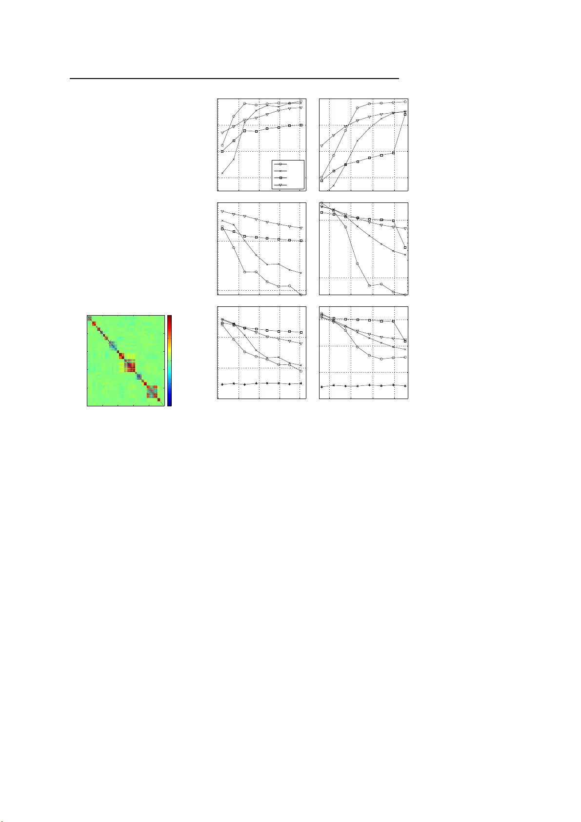
– man uscript No. (will be inserted by the editor) The V ariational Garrote Hilb ert J. K app en · Vicen¸ c G´ omez Receiv ed: date / Accepted: date Abstract In this pap er, we present a new v ariationa l metho d for spa rse re- gressio n using L 0 regular iz ation. The v ariationa l parameters appear in the approximate mo del in a wa y that is similar to Breiman’s Garro te model. W e refer to this metho d as the v ariatio nal Gar rote (VG). W e show that the com- bination of the v ar iational approximation a nd L 0 regular iz ation has the effect of making the problem effectively of max imal r a nk even when the n umber of samples is small compared to the num b er of v ariables. The VG is co mpared nu- merically with the Lasso metho d, r idge regr ession and the recently introduced paired mean field metho d (PMF) [1]. Numerical results show that the V G and PMF yield mor e a ccurate pr e dic tio ns a nd more accura tely reco ns truct the tr ue mo del than the other metho ds. It is shown that the VG finds co rrect so lutions when the Las s o solution is inconsis ten t due to large input co rrelations . Glob- ally , VG is sig nificantly faster than PMF and tends to p erfor m be tter as the problems b ecome denser a nd in pro blems with str ongly cor related inputs. The naive implementation of the VG scales cubic with the num b er of features. By int ro ducing Lagr ange multipliers we obta in a dual for mulation of the problem that scale s cubic in the num b er of samples , but close to linear in the num b er of features. Hilb ert J. Kapp en Donders Institute for Brain Cognition and Beha viour Radboud Universit y Nijmegen 6525 EZ Nij megen, T he Netherlands E-mail: b.k appen@science.ru.nl Vicen¸ c G´ omez Donders Institute for Brain Cognition and Beha viour Radboud Universit y Nijmegen 6525 EZ Nij megen, T he Netherlands E-mail: v.gomez@science.ru.nl 2 Hilb ert J. K appen, Vicen¸ c G´ omez 1 In tro duction One of the mo st common problems in statistics is linear reg ression. Given p samples of n -dimensiona l input data x µ i , i = 1 , . . . , n and 1-dimensional output data y µ , with µ = 1 , . . . , p , find weigh ts w i , w 0 that be st describ e the rela tion y µ = n X i =1 w i x µ i + w 0 + ξ µ (1) for all µ . ξ µ is zero- mea n noise with inv erse v ariance β . The ordina ry least square (OLS) solution is given by w = χ − 1 b a nd w 0 = ¯ y − P i w i ¯ x i , where χ is the input cov aria nce matrix b is the vector o f input- output cov ariances and ¯ x i , ¯ y ar e the mean v alues. There are several problems with the OLS approach. When p is small, it t ypically has a lo w prediction accuracy due to over fitting. In particula r, when p < n , χ is not of maxima l rank and so its inv erse is not uniquely defined. In addition, the OLS solution is not sparse: it will find a so lutio n w i 6 = 0 for all i . There fo re, the interpretation of the OLS solution is often difficult. These problems are well-known, and there exist a num b er of a pproaches to ov er come these pr oblems. The simplest approa ch is called ridge r egressio n. It a dds a regulariza tion ter m 1 2 λ P i w 2 i with λ > 0 to the OL S criter ion. This has the effect that the input cov ar ia nce ma trix χ gets replac e d b y χ + λI which is of max ima l ra nk for all p . One o ptimizes λ by cro ss v alidation. Ridge regres s ion impr ov es the predictio n accur a cy but no t the interpretabilit y of the solution. Another appr oach is La sso [2]. It so lves the OLS problem under the linear constraint P i | w i | ≤ t . This problem is equiv ale n t to a dding an L 1 regular iz a- tion term λ P i | w i | to the OLS cr iter ion. The optimizatio n o f the quadr atic error under linear c o nstraints can be solved efficiently . See [3] for a rec e nt a c- count. Again, λ or t may b e found through cro ss v alida tion. The a dv antage of the L 1 regular iz ation is that the solution tends to b e sparse. This improv es bo th the prediction accuracy and the interpretabilit y o f the solution. The L 1 or L 2 regular iz ation terms are known as shrink age prio rs b eca use their effect is to shrink the size of w i . The idea of shrink a ge prior has b een generalized by [4 ] to the form λ P i | w i | q with q > 0 and q = 1 , 2 co rresp onding to the Lasso a nd r idge case, resp ectively . Better so lutions can be obtained for q < 1, how ever the resulting o ptimiza tion pr oblem is no lo nger conv ex a nd therefore more difficult to solve. An alternative Bayesian approach to obtain a sparse solution using an L 0 pena lty was prop o s ed b y [5]. They intro duce n v ariational selector v ariables s i such that the pr ior distribution over w i is a mixture of a narrow (spike) and wide (slab) Ga ussian distribution, b o th centered on zer o . The p osterio r distribution ov er s i indicates whether the input feature i is included in the mo del or not. Since the num b er of subsets of features is exp onential in n , for large n o ne cannot compute the solution ex actly . In addition, the p oster ior is a co mplex high dimensional distribution of the w i and the other (hyper) The V ariational Garr ote 3 parameters of the mo del. The co mputation of the p oster ior req uires thus the use of MCMC sa mpling [5] or a v ariatio nal Bay esian approximation [1, 6, 7, 8]. Although Bayesian approa ches tend to over fit less than a maximum likeli- ho o d or maximum a p osterio ri metho d (MAP a pproach), they also tend to be relatively s low. Here we prop o se a partial Bay esian a pproach, where we apply a v ariational a pproximation to integrate out the binar y (selecto r) v ariables in combination with a MAP appr oach for the remaining parameter s. F or clarity , we analyse this idea in its mo st simple form, in the absence of (hierarchical) priors. Ins tead, we infer the sparsity pr ior thro ug h cross v alidatio n. As we will motiv ate b elow, we c all the method the V ariatio na l Garrote (V G). The pap er is orga nized as follows. In section 2 we intro duce the mo del and we derive the v ariationa l appr oximation. W e show tha t the combination of the v aria tional approximation and L 0 regular iz ation has the effect of making the problem effectively of maxima l r ank by introducing a ’v a riational ridge ter m’. As a result, the solution is well defined even w he n p < n as long as the num ber of predictive features is less than p (which is controlled by the spar s it y prior). T o g ain further insight, in section 3 we study the case when the design matrix is orthogo nal. In this case the solutio n can b e co mputed exactly in closed for m with no need to reso rt to a pproximations. In the v ariational a p- proximation, we s how for the uni-v ariate cas e that the solution is either unique or ha s tw o so lutions, dep ending on the input-output correla tions, the num ber of s amples p and on the spar sity prio r γ . W e derive a phase plot and show that the s olution is unique , when the sparsity prior is not to o strong or when the input-output cor relation is no t to o large. The input-output b ehavior o f the VG is shown to b e close to optimal as a smo othed version of ha rd featur e selection. W e ar gue that this behavior also holds in the mu lti-v a riate case. In s ection 4 we compar e the VG with a num b er of other MAP metho ds, such as Lasso and ridge reg ression and with the paired mean field metho d (PMF) [1], a rece ntly prop ose d v ariational bayesian metho d. W e show that the VG and P MF significantly outp erform the Las so a nd ridge regres s ion on a lar ge nu mber of different exa mples b oth in ter ms of the accura cy o f the solution, as well as in prediction err or. In a ddition, we show that the VG do not suffer fro m the inc o nsistency of the Lass o metho d when the input correla tio ns are lar ge. W e show in deta il how all metho ds compa re as a function of the level of no ise, the spars it y o f the targe t solution, the num b er of samples and the nu mber of irrelev ant predictors. Globally , VG is significa nt ly faster tha n PMF and tends to p er form b etter as the problems b ecome denser and in pro blems with strongly correla ted inputs. 4 Hilb ert J. K appen, Vicen¸ c G´ omez 2 The v ariational approximation Consider the regr ession mo del of the form 1 y µ = n X i =1 w i s i x µ i + ξ µ n X i =1 s i ≤ t (2) with s i = 0 , 1 . The bits s i = 1 will identify the predictive inputs i . Using a Bay esian des cription, and de no ting the data b y D : { x µ , y µ } , µ = 1 , . . . , p , the likelihoo d term is given by p ( y | x , s , w , β ) = r β 2 π exp   − β 2 y − n X i =1 w i s i x i ! 2   p ( D | s , w , β ) = Y µ p ( y µ | x µ , s , w , β ) =  β 2 π  p/ 2 exp   − β p 2   n X i,j =1 s i s j w i w j χ ij − 2 n X i =1 w i s i b i + σ 2 y     (3) with b i = 1 p P µ x µ i y µ , σ 2 y = 1 p P µ ( y µ ) 2 , χ ij = 1 p P µ x µ i x µ j . W e should als o sp ecify pr ior distributions over s , w , β . F or concreteness , we as sume that the pr ior o ver s is factorized ov er the individual s i , ea ch with ident ical prior proba bility: p ( s | γ ) = n Y i =1 p ( s i | γ ) p ( s i | γ ) = exp ( γ s i ) 1 + exp( γ ) (4) with γ given which sp ecifies the spar sity of the so lution. W e denote by p ( w , β ) the prior o ver the in v erse no ise v ar iance β and the feature weigh ts w . W e will leav e this prio r unsp ecified since its choice do es not affect the v a riational approximation. 2 The p o sterior bec o mes p ( s , w , β | D , γ ) = p ( w , β ) p ( s | γ ) p ( D | s , w , β ) p ( D | γ ) (5) Computing the MAP estimate or computing statistics fr o m the po sterior is complex in particular due to the discrete nature or s . W e prop ose to com- pute a v ar iational approximation to the ma rginal p oster ior p ( w , β | D , γ ) = 1 W e assume fr om here on without loss of generality that 1 p P p µ =1 x µ i = 1 p P p µ =1 y µ = 0 2 It can b e sho wn that the regression mo del s pecified by Eqs. 3 and 4 i s iden tical to the spike and slab mo del, with the difference that the latter usually conta ins a (Gaussian) prior o ver the w i which could also be added in the ab o ve representat ion[1]. See appendix C for details. The V ariational Garr ote 5 P s p ( s , w , β | D , γ ) and computing the MAP solution with resp ect to w , β . Since p ( D | γ ) do es not dep end on w , β we ca n ignore it. The poster ior distribution Eq. 5 for g iven w , β is a typical Boltzmann distribution inv olving terms linear and quadratic in s i . It is well-known that when the effective coupling s w i w j χ ij are small, one can o btain g o o d appr ox- imations using metho ds that orig inated in the sta tistical physics communit y and w he r e s i denote binary s pins . Most prominently , one can use the mean field or v ariational approximation [9], the T AP approximation [1 0] or b elief propaga tion (BP) [11]. F or intro ductions into these metho ds a ls o se e [12, 1 3]. Here, we will develop a so lution base d o n the simplest po s sible v ariational approximation and leav e the p os sible improvemen ts using BP or str uctured mean field approximations to the future. W e a pproximate the sum b y the v aria tio nal b ound using Jens e n’s inequal- it y . log X s p ( s | γ ) p ( D | s , w , β ) ≥ − X s q ( s ) log q ( s ) p ( s | γ ) p ( D | s , w , β ) = − F ( q , w , β ) (6) q ( s ) is c alled the v ar iational appr oximation and can b e any po sitive pr obabil- it y distribution on s a nd F ( q , w , β ) is called the v ar ia tional free ener g y . The optimal q ( s ) is found by minimizing F ( q , w , β ) with res p ect to q ( s ) so that the tightest b ound - b est approximation - is obtained. In or de r to b e a ble to compute the v ariational free energy efficient ly , q ( s ) m ust b e a tr a ctable probability distribution, such as a chain or a tree with limited tr ee-width [14]. Here we consider the simplest case where q ( s ) is a fully factorized distribution: q ( s ) = Q n i =1 q i ( s i ) with q i ( s i ) = m i s i + (1 − m i )(1 − s i ), so that q is fully sp ecified by the exp ected v alues m i = q i ( s i = 1), which we collectively denote by m . The exp ectatio n v alues with resp ect to q can now be easily ev alua ted a nd the r esult is F = β p 2   n X i,j m i m j w i w j χ ij + X i m i (1 − m i ) w 2 i χ ii − 2 n X i =1 m i w i b i + σ 2 y   − γ n X i =1 m i + n X i =1 ( m i log m i + (1 − m i ) lo g(1 − m i )) − p 2 log β 2 π (7) where we have omitted terms indep endent of m, β , w . The fir st line is due to the likelihoo d term, the second line is due to the prior on s a nd the entrop y of q ( s ). The approximate mar g inal p os ter ior is then p ( w , β | D , γ ) ∝ p ( w , β ) X s p ( s | γ ) p ( D | s , w , β ) ≈ p ( w , β ) exp( − F ( m , w , β , γ )) W e can compute the v ariational approximation m for given w , β , γ b y min- imizing F with resp ect to m . In addition, p ( w , β | D , γ ) needs to b e maximized 6 Hilb ert J. K appen, Vicen¸ c G´ omez with resp ect to w , β . Note, tha t the v ar iational approximation only dep ends on the likelihoo d term a nd the prior on γ , since these are the only ter ms that depe nd on s . Thus, for given w , the v ariational appr oximation do es not dep end on the particular c hoices for the prior p ( w , β ). F or concreteness, w e assume a flat prior p ( w , β ) ∝ 1. W e set the deriv atives o f F with r e s pe ct m , w , β equa l to zero. This gives the following set of fixed p oint equa tio ns: m i = σ  γ + β p 2 w 2 i χ ii  (8) w = ( χ ′ ) − 1 b χ ′ ij = χ ij m j + (1 − m j ) χ j j δ ij (9) 1 β = σ 2 y − n X i =1 m i w i b i (10) with σ ( x ) = (1 + exp( − x )) − 1 and where in Eq. 10 we hav e use d E q. 9 . Eqs. 8- 10 pr ovide the final so lution. They can b e solved by fixed p o in t iteration as outlined in Algo rithm 1: Initialize m at ra ndom. Compute w by solving the linear system E q . 9 and β from E q. 10. Compute a new s o lution for m fro m Eq.8. Within the v ariational/ MAP appr oximation the predictive mo del is g iven by y = X i m i w i x i + ξ (11) with  ξ 2  = 1 /β and m , w , β a s es tima ted by the ab ov e pro cedure. Eq. 11 has some similarity with Breiman’s non-nega tive G arr ote metho d [15]. It computes the solution in a t wo step appr o ach: it c o mputes first w i using OLS and then finds m i by minimizing X µ y µ − n X i =1 x µ i w i m i ! 2 sub ject to m i ≥ 0 X i m i ≤ t Because of this similar it y , we refer to our metho d as the v a riational Gar rote (V G). Note, that b ecause of the OLS step the non-negative gar rote req uires that p ≥ n . Instead, the v ariational solutio n Eqs. 8-10 computes the entire solution in one step (and as we will see do es not require p ≥ n ). Let us paus e to make some obs erv atio ns ab out this so lution. One might naively expect that the v a riational approximation w ould simply cons ist of replacing w i s i in Eq. 2 by its v aria tional ex pe c ta tion w i m i . If this were the case, m w ould disa pp e ar entirely from the equations and one would exp ect in Eq. 9 the OLS s olution with the normal input cov ariance matrix χ instea d of the new ma trix χ ′ (note, tha t in the s p ecia l case that m i = 1 for a ll i , χ ′ = χ and Eq. 9 do es r educe to the OLS solution). Instead, m and w ar e b o th to b e optimized, giving in genera l a different so lution than the O L S solution 3 . 3 The technical r eason that this do es not occur is that in the computation of the exp ec- tation with resp ect to the distribution q that results in Eq. 7 one has h s i s j i = m i m j for i 6 = j , but  s 2 i  = h s i i = m i . The V ariational Garr ote 7 When m i < 1 , χ ′ differs fro m χ by resca ling with m i and adding a p o s itive diagonal to it, a ’v ar iational ridge’. This is simila r to the mechanism of ridge regres s ion, but with the impo rtant difference that the diagonal term dep ends on i and is dynamically adjusted dep ending o n the solution for m . Thus, the sparsity prior tog e ther with v ar iational approximation provides a mechanism that solves the ra nk pr o blem. When a ll m i < 1, χ ′ is of max ima l rank. Ea ch m i that a pproaches 1, r educes the rank by o ne. Thus, if χ has rank p < n , χ ′ can b e still o f rank n when no more than p of the m i = 1, the remaining n − p of the m i < 1 ma king up fo r the rank deficiency . Note, that the size of m i (and thu s the ra nk of χ ′ ) is cont rolled by γ through Eq. 8. In the ab ove pro ce dur e, we compute the VG solution for fixed γ and choos e its optimal v a lue through cross v alida tion on independent data [1 6]. This has the adv ant age that our result is indepe ndent of our (po ssibly inco rrect) prior belie f. But a no ther imp orta n t adv antage of v ar ying γ manually is that it helps to av oid lo cal minima. When we increase γ from a negative v alue γ min to a maximal v alue γ max in small steps, we o btain a sequence of so lutions with decreasing spar seness. These solutions will b etter fit the data and a s a result β increases with γ . Thus, increas ing γ implemen ts a n a nnealing mechanism where we sequentially obtain s olutions at low er noise levels. W e found empir- ically that this a pproach is effective to re duce the problem of lo c a l minima. T o further deal with the effect of hysteresis (see sectio n 3) we re c ompute the solution from γ max down to γ min and c ho ose the s o lution with low est free energy . The minimal v alue of γ is chosen a s the la r gest v a lue such tha t m i = ǫ , with ǫ small. W e find fro m E qs. 8-10 that γ min = − pb 2 i χ ii 2 σ 2 y + σ − 1 ( ǫ ) + O ( ǫ ) (12) with σ − 1 ( x ) = log( x/ (1 − x )). W e heuristically set the maxima l v alue of γ a s well as the step size. In a ppe ndix B we provide an alter native fixe d p oint iteratio n scheme that is more efficient in the large n small p limit. Whereas E qs. 8-10 requir e the rep eated so lution of a n -dimensio nal linear system, the dua l fo r mulation, Eqs. (8) ,(21),(24)-(27), requires the r ep eated s o lution o f a p dimensional linear system. Algorithm 1 summarizes the V G metho d. 3 Orthogonal and uni -v ariate case In order to obtain fur ther insight in the solution, conside r the case in which the inputs ar e uncorr elated: χ ij = δ ij . In this cas e , we can derive the MAP so lution of Eq. 5 exactly , without the need to r esort to the v ariationa l approximation. Eq. 5 r educes to a dis tribution that fac to rizes ov er i with lo g pr obability 8 Hilb ert J. K appen, Vicen¸ c G´ omez input : Data D : { x µ , y µ } , µ = 1 , . . . , p ; ǫ and step-size ∆γ output : w , m , β , γ solution wi th minimal cross v alidation error 1 Prepro cess data suc h that P µ x µ i = P µ y µ = 0 and partition D i n D train , D v al 2 Compute b i = 1 p P µ x µ i y µ and if n < p compute χ ij = 1 p P µ x µ i x µ j 3 Compute γ min from ǫ and γ max from γ min and ∆γ 4 for γ = γ min : ∆γ : γ max do // F OR W ARD P ASS 5 η ← 1 6 while not co nver ge d do 7 Compute w , β fr om Eqs. (9)-(10) ( n < p ) or Eqs. (21), (24)-(27) ( n > p ); 8 Compute m ′ using a smo othed version of Eq. (8): m ′ i ← (1 − η ) m i + η σ ( . . . ) 9 if max i | m ′ i − m i | > 0 . 1 then 10 η ← η / 2 11 m ← m ′ 12 Store solution ( w 1 , m 1 , β 1 ) γ and F 1 ( γ ) ← F (( w 1 , m 1 , β 1 ) γ ) from Eq. (7) 13 for γ = γ max : − ∆γ : γ min do // BACKW ARD P ASS 14 As 5 − 11 15 Store solution ( w 2 , m 2 , β 2 ) γ and F 2 ( γ ) ← F (( w 2 , m 2 , β 2 ) γ ) from Eq. (7) 16 for γ = γ min : ∆γ : γ max do 17 Choose solution ( w , m , β ) γ that has minimal F 1 , 2 ( γ ) 18 Compute cross v ali dation error on D v al using Eq. (11) 19 Select w , m , β , γ wi th minimal cross v alidation error Algorithm 1: The V a riational Garrote algorithm. prop ortiona l to L = p 2 log β − β p 2 n X i =1 s i ( w 2 i − 2 w i b i ) + σ 2 y ! + γ n X i =1 s i Maximizing wrt w i , β yields w i = b i , β − 1 = σ 2 y − P n i =1 s i b 2 i and L = p 2 log β + n X i =1 s i  β p 2 b 2 i + γ  − β p 2 σ 2 y Assume without los s of generality that b 2 i are sorted in decreas ing order. L is maximized by setting s i = 1 w he n β p 2 b 2 i + γ > 0 and s i = 0 o therwise. Thus, the o ptimal s olution is s 1: k = 1 , s k +1: n = 0 , β − 1 = σ 2 y − P k i =1 b 2 i with k the smallest in teger such that β p 2 b 2 k +1 + γ < 0 (13) By v a r ying γ from small to lar ge, we find a sequence of solutions with decreas - ing sparsity . In the v a riational a pproximation the s o lution is very similar but no t iden- tical. Eq. 9 gives the same solution w i = b i . Eqs. 8 and 10 beco me m i = σ  γ + β p 2 b 2 i  1 /β = σ 2 y − X i b 2 i m i The V ariational Garr ote 9 which we can interpret as the v a riational a pproximations of E q. 1 3, with m 1: k ≈ 1 a nd m k +1: n ≈ 0. The term P i b 2 i m i is the expla ined v aria nce and is subtracted from the total o utput v ar ia nce to give a n e s timate of the no ise v aria nce 1 / β . Note that the po sterior is factorized in s i , the v a riational approximation is not ident ical to the exa ct map solutio n Eq. 1 3, a lthough the results are very similar. The relation is s i = 0 ⇔ m i < 0 . 5 and s i = 1 ⇔ m i > 0 . 5. In o rder to fur ther analyze the v ariational solution, we consider the 1- dimensional case. The v a r iational equations b eco me m = σ  γ + p 2 ρ 1 − ρm  = f ( m ) (14) 1 β = σ 2 y (1 − mρ ) (15) with ρ = b 2 /σ 2 y the squared corr elation co efficient. In Eq. 14, we have eliminated β and w e must find a s o lution for m fo r this non-linear equation. W e see tha t it dep ends o n the input-output co rrelation ρ , the num ber o f s amples p and the s parsity γ . F or p = 100, the solution for different ρ, γ is illustra ted in fig ure 10 (see app endix A). E q. 14 ha s o ne o r three so lutions for m , de p ending on the v alues o f γ , ρ, p . The thr e e solutions corres p o nd to tw o lo cal minima and one lo cal maximum o f the free energ y F . F or γ = − 40 and γ = − 1 0, we plot the stable solution(s) for different v alues of ρ in the ins e rts in fig. 1. The b est v aria tio nal so lution for m is given by the solution with the low est free energ y , indicated b y the so lid lines in the inser ts in fig. 1. Fig. 1 further shows the phas e plot of γ , ρ that indica tes that the v ariational solution is unique fo r γ > γ ∗ or for ρ < ρ ∗ . The solid line for 0 < ρ < ρ ∗ in fig. 1 indicates a smo o th (second order) pha s e transition from m = 0 to m = 1. F or ρ > ρ ∗ , the transition fr o m m = 0 to m = 1 is dis contin uo us: for each ρ there is a ra nge of v a lue s o f γ where tw o v ariationa l so lutions m ≈ 0 and m ≈ 1 co-exist. F or comparison, w e also show the line γ = − pρ/ 2 that s e pa rates the solution s = 0 and s = 1 acco rding the the exact (non-v ar iational) solution Eq. 13. The multi-v alued v ariational solution results in a hysteresis e ffect. When the s olution is computed for incre asing γ , the m ≈ 0 solution is obtained until it no longer exists. If the s equence of solutions is computed for dec reasing γ the m ≈ 1 so lution is obtained for v alues of γ where pre v iously the m ≈ 0 solution was obtained. F rom this simple o ne-dimensional cas e we may infer that the v ariational approximation is re la tively easy to co mpute in the uni-mo dal regio n (small ρ or γ not to o negative) and b eco mes more ina ccurate in the regio n where m ultiple minima exist (region b etw een the dot-da s hed a nd dashed lines in fig. 1) . It is interesting to co mpare the uni-v ariate solution of the v ariationa l gar - rote with r idge reg ression, Lasso or Br eiman’s Garro te, which was previo usly done for the latter three metho ds in [2]. Supp ose that data are generated fro m 10 Hilb ert J. K appen, Vicen¸ c G´ omez 0 0.2 0.4 0.6 0.8 1 −80 −70 −60 −50 −40 −30 −20 −10 0 ρ γ 0 0.5 1 0 0.5 1 ρ m 0 0.5 1 0 0.5 1 ρ m Fig. 1 Phase plot ρ, γ for p = 100 giving the different solutions for m . Dashed and dot- dashed lines for ρ > ρ ∗ = 0 . 28 ar e from Eq. 18 where t wo solutions for m exist. Solid li ne for ρ < ρ ∗ is the solution for γ when m = 1 / 2, to indicate the transition from the unique solution m ≈ 0 to the unique solution m ≈ 1. Dotted line is the exact transition from s = 0 to s = 1 from Eq. 13. Insets indicate solutions for m versus ρ for γ = − 10 , p = 100 (top-righ t) and for γ = − 40 , p = 100 (bottom-left). In the low er left corner of the insets, the unique solution m ≈ 0 is found. In the top right corner, the unique solution m ≈ 1 is found. Betw een the dot-dashed and the dashed l ine, the tw o v ariational solutions m ≈ 0 and m ≈ 1 co-exist. the mo del y = wx + ξ with  ξ 2  =  x 2  = 1. W e co mpare the s olutions as a function o f w . The OL S solution is approximately given by w ols ≈ h xy i = w , where we ignor e the statistical deviations of or der 1 /p due to the finite data set size. Similarly , the ridge regr ession solution is given b y w ridge ≈ λw , with 0 < λ < 1 dep ending o n the r idge prior. The Lasso solution (for non-nega tive w ) is g iven by w lasso = ( w − γ ) + [2], with γ dep ending on the L 1 constraint. Breiman’s Gar rote so lution is given by w garrote = (1 − γ w 2 ) + w [2], with γ de- pending on the L 1 constraint. The VG solutio n is g iven by w vg = mw , with m the solutio n of Eq . 14. Note, that the VG solution dep ends, in addition to w, γ , on the unex plained v aria nce σ 2 y and the num b er of sa mples p , wherea s the other metho ds do not. The qualita tive difference of the solutions is shown in fig. 2. The ridge regres s ion solution is off by a constant multip licative factor . The Lasso solution is zero for small w and for larg er w gives a solution that is shifted down wards by a c o nstant factor. B r eiman’s Garrote is identical to the La sso for small w and shrinks less for larger w . The V G gives an almost ideal behavior and can be int erpreted as a so ft v ersio n of v ar iable selection: F or small w the solution is clo se to zero a nd the v ar ia ble is igno red, and ab ov e a thres hold it is identical to the OLS solution. The V ariational Garr ote 11 0 0.5 1 1.5 0 0.5 1 1.5 w w estimated vg ridge garrote lasso Fig. 2 Uni-v ariate solution for different r egression methods. All methods yield a shrinke d solution (deviation fr om di agonal line). V ariational Garr ote (VG ) with γ = − 10 , p = 100 and σ 2 y = 1. R i dge r egression with λ = 0 . 5. Garrote with γ = 1 / 4. Lasso with γ = 1 / 2. The q ua litative natur e of the phase plot fig. 1 and the input-o utput b e- havior fig. 2 extends to the multi-v ariate orthog onal case. The symmetry breaking o f feature i is indep endent of all other features, ex cept for the ter m δ = P j 6 = i b 2 j m j that enters through β . If we increas e γ , δ increas e s in steps each time that o ne of the features j switches from m j ≈ 0 to m j ≈ 1 . Thus δ is cons tant a lmost a lwa ys, e x cept at the step p o ints. Since the cr itical v alues of ρ and γ dep e nd in a simple wa y on δ , the pha se plot for the mult iv a riate orthogo nal case is qualitatively the same as for the uni-v ariate case. 4 Numerical example s In the following exa mples, we compare the VG with Las so, r idge regres sion and in some cases, with the paired mean field approach (PMF) [1]. F or most of the examples, we generate a training set, a v alidation set and a tes t s et. Inputs a re generated from a ze r o mea n m ulti-v a riate Ga ussian distribution with sp ecified cov ar iance structure. W e generate outputs y µ = P i ˆ w i x µ i + dξ µ with dξ µ ∈ N (0 , ˆ σ ) a nd ˆ w i depe nding on the problem. F or V G, ridg e regre s sion and La sso, we o ptimize the model pa r ameters on the training set and, when necessary , o ptimize the hyper parameter s ( γ in the cas e o f VG, λ in the case o f ridge re g ression and Lasso) that minimize the quadr a tic err or on the v a lidation s e t. F or the Lasso , we used the metho d describ ed in [3] 4 . 4 http://w ww- stat.stanford.edu/ ~ tibs/glm net- matlab/ . 12 Hilb ert J. K appen, Vicen¸ c G´ omez Compariso n with P MF is p erfor med using the soft ware av ailable online for the regres s ion case with o ne-dimensional output 5 . Since P MF o ptimizes hyperpara meters as well, we merg e b oth training and v a lidation sets and the resulting datas et is used a s input for the PMF metho d. This ensures that all metho ds use the same data for parameter estimation. W e define the solution vector for a given metho d as v . F or VG, the co mpo - nent s are v i ≡ m i w i . In the case of PMF, m i corres p o nds to the spike-and-slab v aria tional po sterior and w i to the v ariational mean for the weigh ts 6 . F or Ridge and Lasso v i ≡ w i . 4.1 Small Example 1 In the first example, we take indep endent inputs x µ i ∈ N (0 , 1) and a teacher weigh t vector with only one non- zero ent ry: ˆ w = (1 , 0 , . . . , 0), n = 10 0 and ˆ σ = 1 . The tr aining set size p = 5 0 , v alidation set size p v = 50 and test se t size p t = 4 0 0. W e choo se ǫ = 0 . 001 in E q. 12, γ max = 0 . 0 2 γ min , ∆γ = − 0 . 02 γ min (see Algorithm 1 for details). Results for a single run o f the V G are shown in fig. 3. In fig. 3 a , we plot the minimal v ariational free ener gy F versus γ for b oth the forward and backw ard run. Note, the h ysteresis effect due to the lo cal minima . F or each γ , we use the solution with the low est F . In fig. 3b, we plot the training error and v alidation error versus γ . The optimal γ ≈ − 2 1 is denoted by a star and the cor resp onding σ = 1 / √ β = 1 . 05 . In fig. 3c, w e plot the non- z ero c omp onent v 1 = m 1 w 1 and the ma x im um abs olute v alue of the remaining compo nent s versus γ . Note the robustness of the VG s o lution in the sense of the larg e range o f γ v a lues for which the correct solution is found. In fig. 3d, we plot the o ptimal so lution v i = m i w i versus i . In fig . 4 we show the Lasso (top row) and ridge regr ession (b ottom row) results for the same da ta set. The optimal v alue for λ minimizes the v alidation error (star). In fig . 4b,c we see that the Lasso selects a num ber of inc o rrect features a s well. Fig . 4b als o shows that the La sso solution w ith a larger λ in the range 0 . 45 < λ < 0 . 95 could select the sing le cor rect featur e, but would then es tima te ˆ w 1 to o small due to the lar ge shrink age effect. Ridge regre ssion gives very bad results. The non-zero fea ture is to o small and the r emaining features hav e large v alue s . Note from fig . 4e, that r idge regress ion yields a non-spars e solution for all v alue s of λ . T able 1 shows tha t the VG s ignificantly outp erforms the L a sso metho d and ridge r e gressio n b oth in terms o f prediction erro r, the accura cy of the estimation of the par ameters and the n umber of non-zero par ameters. In this simple example, there is no significa nt difference in the prediction erro r of Lasso, P MF and VG, but the Lasso solution is significantly les s sparse . There is no significant difference b etw e e n the solutions found b y PMF and VG. 5 http://w ww.well.ox. ac.uk/ ~ mtitsias /software.h tml . 6 The notation in [1] uses ˜ w i for w i and γ i for m i . The V ariational Garr ote 13 −30 −20 −10 0 0 10 20 30 40 50 60 γ F (a) forward backward −30 −20 −10 0 0.5 1 1.5 2 2.5 error γ (b) train val −30 −20 −10 0 0 0.5 1 1.5 2 γ (c) v 1 max |v(2:n)| 1 50 100 0 0.5 1 v component (d) Fig. 3 T op left (a): Minim al v ar iational free energy versus γ . The tw o curves corr espond to wa rm start solution f rom small to large γ (’forward’) and from large to smal l γ (’bac kward’) (see also Algorithm 1 ). T op ri gh t (b): T raining and v ali dation error versus γ . The optimal γ minimizes the v alidation error. Bottom l ef t (c): Solution v 1 = m 1 w 1 and max i =2: n | m i w i | . The correct solution is found in the range γ ≈ − 20 to γ ≈ − 5. Bottom ri gh t (d): Optimal solution v i = w i m i v ersus i . T rain V al T est # non-zero k δ v k 1 Ridge 0 . 60 ± 0 . 43 1 . 72 ± 0 . 39 1 . 80 ± 0 . 12 − 3 . 97 ± 1 . 23 Lasso 0 . 78 ± 0 . 26 1 . 07 ± 0 . 20 1 . 17 ± 0 . 20 8 . 65 ± 6 . 75 0 . 80 ± 0 . 57 PMF − − 1 . 02 ± 0 . 10 1 . 5 ± 1 . 19 0 . 33 ± 0 . 37 VG 0 . 85 ± 0 . 22 0 . 96 ± 0 . 17 1 . 01 ± 0 . 10 1 . 20 ± 0 . 52 0 . 31 ± 0 . 30 T rue 0 . 93 ± 0 . 14 0 . 87 ± 0 . 20 0 . 98 ± 0 . 04 1 0 T able 1 Results for Example 1 av eraged ov er 20 instances. T rain i s mean squared error (MSE) on the training s et. V al is MSE on the v alidation set. T est is MSE on the test s et. # non-zero is the n umber of non-zero elements in the Lasso solution and P n i =1 ( m i > 0 . 5) for VG and PMF. k δ v k 1 = P n i =1 | v i − ˆ w i | . 4.2 Small Example 2 In the second example, we conside r the effect o f co rrelations in the input dis- tribution. F o llowing [2] we genera te input data from a m ulti-v ar iate Gaus sian distribution with cov ar ia nce matrix χ ij = ζ | i − j | , with ζ = 0 . 5. In a ddition, we choose multiple fea tures non-z ero: ˆ w i = 1 , i = 1 , 2 , 5 , 10 , 50 and all other ˆ w i = 0. W e use n = 100 , ˆ σ = 1 and p/ p v /p t = 50 / 50 / 400. In table 2 we compare the perfor ma nce of the VG, La sso, ridge regression and PMF on 14 Hilb ert J. K appen, Vicen¸ c G´ omez 0 0.5 1 1.5 0 0.5 1 1.5 2 2.5 3 λ error (a) train val 0 0.5 1 1.5 0 0.2 0.4 0.6 0.8 1 λ (b) v 1 max |v(2:n)| 1 50 100 0 0.5 1 i v i (c) Lasso 0 5 10 0 0.5 1 1.5 2 2.5 3 λ error (d) train val 0 5 10 0 0.2 0.4 0.6 0.8 1 λ (e) v 1 max |v(2:n)| 1 50 100 0 0.5 1 i v i (f) Ridge Regression Fig. 4 R egressi on solution for Lasso and r idge regression for same data set as in fig. 3. T op row (a,b,c): Lasso. Bottom row (d,e,f ): Ridge regression. Left column (a,d): training and v alidation err ors versus λ . Mi ddle column (b,e): Solution f or the non-zero f eature v 1 and the zero-features max i =2: n | v i | . Right column (c,f ): Optimal Lasso and r idge regression solution v i v ersus i . T rain V al T est # non-zero k δ v k 1 Ridge 0 . 32 ± 0 . 27 3 . 30 ± 0 . 67 3 . 46 ± 0 . 31 − 11 . 09 ± 0 . 93 Lasso 0 . 75 ± 0 . 37 1 . 39 ± 0 . 37 1 . 48 ± 0 . 29 16 . 30 ± 6 . 60 2 . 08 ± 0 . 87 PMF − − 1 . 06 ± 0 . 11 5 . 15 ± 0 . 49 0 . 67 ± 0 . 35 VG 0 . 80 ± 0 . 25 1 . 13 ± 0 . 31 1 . 15 ± 0 . 21 5 . 05 ± 0 . 51 0 . 83 ± 0 . 54 T rue 0 . 93 ± 0 . 14 0 . 87 ± 0 . 20 0 . 98 ± 0 . 04 5 0 T able 2 Results for Example 2. F or definitions see caption of T able 1 abov e. 20 ra ndo m instances. W e see that the VG and P MF significa nt ly outp erfor m the Lasso metho d and ridg e re g ression bo th in terms of predictio n e rror and accuracy o f the estimation of the par ameters. Again, ther e is no significant difference b etw e en P MF and V G. 4.3 Effect of the noise In this subsection we show the accuracy VG, Lasso and PMF a s a function of the noise ˆ σ 2 . W e genera te data with n = 100 , p = 10 0 , p v = 20 and ˆ w i = 1 for 20 rando mly chosen comp onents i . W e v a r y ˆ σ 2 in the r a nge 10 − 4 to 10 for for t wo v alues of the correlatio n strength in the inputs ζ = 0 . 5 , 0 . 95. F or weakly correla ted inputs, Fig . 5a., we distinguish three no ise domains: for large noise all metho ds pro duce err ors of O (1) and fail to find the pr edictive The V ariational Garr ote 15 10 −4 10 −3 10 −2 10 −1 10 0 10 1 10 −4 10 −3 10 −2 10 −1 10 0 10 1 σ 2 || δ v || 1 corr = 0.50 (a) VG Lasso PMF 10 −4 10 −3 10 −2 10 −1 10 0 10 1 10 −4 10 −3 10 −2 10 −1 10 0 10 1 σ 2 || δ v || 1 corr = 0.95 (b) VG Lasso PMF Fig. 5 Accuracy of V G, Lasso and P M F as a f unction of the noise. Errorbars of k δ v k 1 for 10 differen t random instances. Data is generated using n = 100 , p = 100 , p v = 20 and ˆ w i = 1 for 20 randomly chose n comp onen ts i . W e consider t wo v alues of the correlation strength i n the inputs: (a) weakly corr elated inputs ζ = 0 . 5 and (b) strongly correlated inputs ζ = 0 . 95. F or PMF we choose the b est solution (the one with highest v alue of the bound) for 10 differen t random initializations for eac h of the 10 instances. features. F or intermediate and low nois e lev els, V G and P MF a re significantly better than Lasso . In the limit of zero noise, the err or of VG and PMF keeps on decreasing whereas the Lasso error saturates to a constant v alue. F or s tr ongly cor related inputs, Fig . 5b., w e obs erve that whereas the er ror of V G scales approximately as befor e, PMF gets stuck in lo c a l minima in some instances, yielding worse average p er formance tha n VG. See section 5 for a further discussion of this po int. 4.4 Analysis of consistency: V G vs Lasso It is well-known that the Lasso metho d may yield inconsistent r esults when input v ariables are co rrelated. In [17], necessa ry and sufficient conditio ns for consistency are der ived. In addition, they give a num b e r of e x amples wher e Lasso gives inconsistent r esults. Their simplest exa mple has three input v ari- ables, x 1 , x 2 , x 3 . x 1 , x 2 , ξ , e a r e indep e nden t and Nor ma l dis tributed rando m v aria bles, x 3 = 2 / 3 x 1 + 2 / 3 x 2 + ξ and y = P 3 i =1 ˆ w i x i + e , p = 1000 . When ˆ w = ( − 2 , 3 , 0) (Example b) this exa mple is consistent, but when ˆ w = (2 , 3 , 0 ) (Example a ) this example violates the consis tency condition. The La sso and V G solution for Ex a mple a for different v alues of λ a nd γ ar e s hown in fig. 6a,b, resp ectively . The VG solutio n v i = m i w i in terms of m i and w i is shown in fig. 6 c ,d. The av erag e results ov er 100 ins ta nces for Ex ample a and Example b are shown in ta ble 3. W e see that the VG do es no t s uffer from inco nsistency and always finds the c o rrect solutio n. This is remark able as one might hav e feared tha t the non-conv exity of the V G w ould result in sub-optimal local minima. 16 Hilb ert J. K appen, Vicen¸ c G´ omez 0 1 2 3 4 0 0.5 1 1.5 2 2.5 3 3.5 λ w w 1 w 2 w 3 −8 −6 −4 −2 0 0 0.5 1 1.5 2 2.5 3 3.5 −log(− γ ) v v 1 v 2 v 3 −8 −6 −4 −2 0 0 0.5 1 1.5 −log(− γ ) m m 1 m 2 m 3 −8 −6 −4 −2 0 0 0.5 1 1.5 2 2.5 3 3.5 −log(− γ ) w w 1 w 2 w 3 Fig. 6 (Color onli ne) Lasso and VG solution for the inconsistent Example a of [17]. T op left: Lasso solution versus λ is call ed inconsisten t b ecause i t do es not contain a λ for which the correct sparsi ty ( w 1 , 2 6 = 0 , w 3 = 0) is obtained. T op r igh t: the VG solution for v versus γ con tains large r ange of γ for which the correct s ol ution is obtained. Bottom l ef t: VG solution for m (curves for m 1 , 2 are identical). Bottom right: VG solution for w . Example a Example b k δ v k 1 max( | v 3 | ) k δ v k 1 max( | v 3 | ) Ridge 0 . 64 ± 0 . 18 0 . 48 0 . 02 ± 0 . 02 0 . 27 Lasso 0 . 19 ± 0 . 14 0 . 30 0 . 00 ± 0 . 00 0 . 00 VG 0 . 05 ± 0 . 03 0 . 00 0 . 00 ± 0 . 00 0 . 00 T able 3 Accuracy of Ridge, Lasso and VG for Example 1a,b fr om [17]. p = p v = 1000. Pa rameters λ (Ridge and Lasso) and γ (VG) optimized through cross v alidation. k δ v k 1 as b efore, max( | v 3 | ) i s maximum ov er 100 trials of the absolute v alue of v 3 . Example a is inconsisten t f or Lasso and yields muc h larger errors than the VG. Example b is consisten t and the qualit y of the Lasso and VG are simi lar. Ridge regressi on i s bad for b oth examples. 4.5 Boston-ho us ing dataset: VG vs PMF W e now fo cus on comparing in more detail the pe r formance o f VG with P MF. In [1 ], the Boston-ho using dataset 7 is used to test the accura c y of the PMF approximation. This is a linear regress ion problem that co nsists of 4 56 training examples with o ne-dimensional r esp onse v ar ia ble y and 13 pre dic to rs that include hous- ing v alues. W e use here the s ame s e tup as in [1] to compare VG with PMF. F or PMF, hyper parameters were fixed to v alues σ = 0 . 1 × v ar ( y ) , π = 0 . 25 , σ w = 1 7 http://a rchive.ics. uci.edu/ml/datasets/Housing The V ariational Garr ote 17 soft - error extr eme - error PMF [1] 0.208 [0.002, 0.454] 0.204 [ 0.002, 0.454] PMF 0.237 [0. 001, 0.454] 0.209 [0.001, 0.454] VG 0.006 [0. 006, 0.006] 0.006 [0.006, 0.006] T able 4 Comparison of VG and PMF i n the Boston-housing dataset in terms of appro xi- mating the ground-truth ˆ w . A verage err ors k δ v k 1 = P n i =1 | v i − ˆ w i | , wi th v i the approxima- tion of VG or PM F, together with 95% confidence interv als (given by per centiles) obtained after 300 r andom initializations for b oth soft and extreme initializations. where v ar(y) denotes the output v ariance. F or the V G, we use β = 1 / σ 2 , γ = log( π / (1 − π )) a nd h yp erpar ameter σ w is implicitly equal to ∞ in the VG (see App e ndix C for details of how b oth mo dels compar e). Since γ and β ar e given, the VG alg orithm reduce s to iter ate eqs. (8) and (9 ) starting fr om a random m . Similar ly , the PMF reduces to p erform an E-step given the fixe d hyperpara meter v alues. As in [1], we use ra ndo m initial v a lues for the v ariational par ameters b e- twe en 0 and 1 ( soft initia lization) and ra ndo m v alues e qu al t o 0 or 1 ( har d initialization). W e cons ide r ed as gro und truth ˆ w ≡ w tr the result of the effi- cient paired Gibbs sampler developed in [1]. T able 4 shows the r esults. The first and seco nd r ows show the error s re - po rted in [1] and the error s that we obtain using their so ft ware, resp ectively . W e o bserve a s mall discr epancy in the av erage error s. How ever, if w e consider the p ercentiles, the r e s ults are consistent. In prac tice, wha t we observe is that PMF finds tw o lo ca l optima dep ending on the initialization: one is the cor rect solution (err or ≈ 10 − 3 ) where a s the other has error 0 . 454. These t wo s o lu- tions are fo und equally o ften for b oth soft o r hard initia liz ations, showing no depe ndence on the t yp e of initialization, in ag reement with [1 ]. The results of V G are shown on the third row. Contrary to PMF, the V G shows no dependence on the initializa tion and always finds a so lution with an err or o f order 10 − 3 . These r esults give evidence that the combined v aria tional/MAP approach o f V G can b e b etter tha n PMF av oiding loca l minima. 4.6 Dependence on the Num be r of Samples W e now analyze the p er formance of all considered metho ds as a function of the prop ortion of samples av aila ble. W e firs t analyze the case when inputs are no t correla ted and then consider c orrela tio ns of pr a ctical r elev anc e that app ea r in genetic datasets. F or these exp er iments, we genera te the data for dimension n = 50 0 and noise level β = 1. W e explore t wo scenario s: very spa rse problems with only 10% o f active pre dictors and denser pr oblems with 25% of active pr edictors. The weigh ts of the active pr edictors are set to 1. 18 Hilb ert J. K appen, Vicen¸ c G´ omez 0.2 0.3 0.4 0.5 0.6 0.5 0.6 0.7 0.8 0.9 1 area under ROC curve sparsity = 10% VG PMF Lasso Ridge 0.2 0.3 0.4 0.5 0.6 10 −2 10 −1 10 0 reconstruction error 0.2 0.3 0.4 0.5 0.6 10 −1 10 1 10 3 10 5 generalization error proportion examples (p/n) 0.4 0.6 0.8 1 0.5 0.6 0.7 0.8 0.9 1 sparsity = 25% 0.4 0.6 0.8 1 10 −1 10 0 10 1 0.4 0.6 0.8 1 10 −1 10 1 10 3 10 5 proportion examples (p/n) Fig. 7 Uncorrelated c ase : P erformance as a function of num ber of training sampl es p for t wo levels of sparsity (10% and 25% of non-zero entries). F or each v alue av erages ov er 20 runs are pl otted. T op: area under the ROC curves (see text for definition). Middle: recon- struction error, defined as k δ v k 1 = P n i =1 | v i − ˆ w i | . Bott om: generalization err or, defined as the MSE in the test set. F or al l methods except for PMF, train set size is p and v ali- dation s ets size p v = p/ 30. F or PMF the training set has si ze p + p v . Low est curv e shows theoretically optimal generalization error obtained by using the target weigh ts from which the data is generated. 4.6.1 Unc orr elate d Case Figure 7 shows r esults o f p er formance for uncorrelated inputs. T op plots show the a rea under the Receiver Op er ating Chara cteristic (ROC) curve. The R OC curve is calc ula ted by thresho lding the weigh t estimates. Those weights that lie ab ove (be low) the thres hold are consider ed as active (inac tive) predictor s. The ROC curve plots the fraction of true p ositives versus the fraction o f fals e po sitives for a ll threshold v alues. The a rea under the curve mea sures the a bil- it y o f the metho d to co rrectly classify those predicto rs that are and are not The V ariational Garr ote 19 active. A v alue of 1 for the area repre s ents a perfect classification wherea s 0.5 repr esents random class ifica tion. The ROC is plotted as a function of the fraction of samples relative to the num b er of inputs: p/n . F or bo th VG and PMF, we observe in all p e r formance mea sures a tr ansi- tion from a r egime where so lutions a re p o or to a regime with a lmost p erfect recov ery . T his transition, not no ticeable in the other (convex) metho ds, o c- curs at around 3 5% of e xamples for 1 0% of sparsity (left column) and shifts to higher v alues for denser proble ms ( ≈ 6 0% for 25% of spa rsity , right column). If we co mpare VG with PMF we see that in the reg ime wher e b oth metho ds per form well, PMF p erfor ms slightly b etter than V G in terms o f reconstruc- tion erro r but their p erfo rmance is identical in terms of the area under the R OC cur ve. The differ ence b etw e e n VG and PMF is slightly mor e pronounced for denser problems. W e also see that La sso p erforms b etter than Ridge r e gres- sion, but the difference betw een b o th metho ds tends to b e smaller for denser problems. Both Lasso and ridge regres sion ar e significantly worse than VG and PMF. 4.6.2 Corr elate d c ase: Genetic dataset W e now consider cor related inputs. W e use input da ta o btained from a ge- netic domain, where inputs x i denote single nucleotide p olymorphisms (SNPs) that hav e v alues x i = { 0 , 1 , 2 } . SNPs typically show corre lations structure d in blo cks, where near by SNPs are highly c o rrelated, but show no dep endence on distant SNPs. An exa mple o f such cor relation matr ix can be seen in Figure 8 (left). The output data are generated as ab ov e. Figure 8 (rig ht ) shows the r esults. Co ntrary to the uncorr elated case, the existence of strong correla tions b etw een some of the predictors preven ts a clear dis tinction b etw e e n so lution r egimes as a function of training set size. W e obser ve, as b efore , that b oth VG and PMF ar e the prefera ble metho ds for sufficiently large training set size. In the thr e e p erfor mance mea sures cons id- ered, VG p e rforms better or co mparable to PMF. Interestingly , the difference betw een VG and P MF b ecomes more significant for denser problems, when we exp ect more difficulty due to more presence of lo cal minima. 4.7 Scaling with dimension n W e conclude our empiric al study by analy zing how the metho ds sca le, b oth in terms of the quality of the so lution as in terms o f CPU times, as a function of the num b er of features n for a co nstant num b er of samples . W e us e the data as in Example 2 ab ov e, with uncorr elated inputs. Figure 9 shows the re sults for VG, PMF and Las s o. F or the VG, we use the dual method desc r ib ed in the a ppendix B. Fig. 9a shows that the V G and PMF hav e constant qualit y in terms o f the error k δ v k 1 , whereas the quality of the Lasso deterior a tes with n . Fig. 9b shows that the VG and P MF hav e close to optimal nor ms L 0 = 5 a nd that the L 0 norm of the Lasso 20 Hilb ert J. K appen, Vicen¸ c G´ omez Correlation between predictors 100 200 300 400 500 100 200 300 400 500 −1 −0.5 0 0.5 1 0.2 0.3 0.4 0.5 0.6 0.7 0.8 0.9 1 area under ROC curve sparsity = 10% VG PMF Lasso Ridge 0.2 0.3 0.4 0.5 0.6 10 −1 10 0 reconstruction error 0.2 0.3 0.4 0.5 0.6 10 −1 10 1 10 3 10 5 generalization error proportion examples (p/n) 0.4 0.6 0.8 1 0.7 0.8 0.9 1 sparsity = 25% 0.4 0.6 0.8 1 10 0 10 1 0.4 0.6 0.8 1 10 −1 10 1 10 3 10 5 proportion examples (p/n) Fig. 8 Correlat ed ca se : (LEFT) (Color online) Example of input correlation m atri x. (RIGHT) P erformance as a function of nu mber of training samples p for t wo levels of sparsity (10% and 25% of non-zero entries). F or each v alue av erages ov er 20 runs are plotted. T op: area under the ROC curves (see text for definition). Mi ddle: reconstruction error, defined as k δ v k 1 = P n i =1 | v i − ˆ w i | . Bo ttom: generalization error, defined as the MSE in the v alidation set. F or all m ethods except for PMF, train set size is p and v al i dation sets size p v = p/ 10. F or PMF the traini ng set has size p + p v . deteriorates with n . Fig. 9c shows that the computation time of all metho ds scales approximately linear with n . Lasso is significantly faster than VG and PMF, and VG is sig nificantly fas ter than PMF. Note, how ev er that the VG and the PMF methods are implement ed in Matlab whereas the Lasso metho d uses an optimized F ortran implementation. The V ariational Garr ote 21 10 2 10 3 10 4 0 1 2 3 4 n || δ v || 1 (a) VG PMF (dual) Lasso 10 2 10 3 10 4 0 10 20 30 40 50 60 n L 0 (b) 10 2 10 3 10 4 10 −2 10 −1 10 0 10 1 10 2 10 3 n cpu−time (c) Fig. 9 Scaling with n : p erformance of VG, PM F and Lasso as a function of the num b er of features n . Data are generated as in Example 2. p = 100 , p v = 100 , β = 2 , ζ = 0. 5 Discussion In this pap er, we hav e intro duced a new v a riational metho d for spa rse regres- sion us ing L 0 pena lty . W e hav e presented a minimal version of the mo del with no (hiera rchical) prior distributions to highlight so me imp ortant feature s: the v aria tional ridge term that dynamica lly regula rizes the regres sion; the input- output behavior a s a smo othed version of hard featur e s election; a phase plot that shows when the v ariational so lution is unique in the or tho gonal desig n cas e for different p, ρ, γ . W e have a lso shown num erically that the VG is efficie nt and accurate a nd yields res ults that significa n tly o utper form other co nsidered metho ds. The V G suffers fro m local minima a s can b e exp ected for a ny method that needs to solve a non-conv ex pro blem, lik e the PMF. F r om the n umerical exp eriments w e c a n conclude tha t VG is o n average preferable to PMF in practical scena rios with strongly corr elated inputs and/ o r mo derately sparse problems, where the lo cal minima problem is more severe. Although we hav e no principled so lution for the lo cal minima problem, we think that the com- bined v a r iational/MAP approach together with the the annealing pro cedure that results from incr e asing γ , followed by a ”heating” phas e to detect hys- teresis works well in pra c tice , helping to av oid lo ca l minima. Another obvious approach is to use multiple re starts or using more p owerful appr oximations, such as structured mean field a pproximation or b elief pro pa gation. W e remar k that the PMF in the general setting [1] includes a n extr a lay er of flexibility that can b e used to capture corr elations b etw ee n input v ariables. Such ex tens ions can also be considered for V G. W e hav e no t e x plored the us e of different priors on w or o n β . In a ddition, a prior could b e imp o sed on γ . It is likely that for particular pro blems the use of a suitable prior could further improv e the r esults. W e have seen that the p erfor mance o f the VG is excellent in the zer o no ise limit. In this limit, the regress ion pro blem r educes to a c o mpressed sensing 22 Hilb ert J. K appen, Vicen¸ c G´ omez problem [18, 19]. The p erfo rmance o f co mpressed sensing w ith L q sparseness pena lty was ana ly zed theoretically in [20], showing the s upe r iority of the L 1 pena lty in c omparison to the L 2 pena lty and suggesting the optimality of the L 0 pena lty . Our numerical r esult are in a greement with this finding. Our implementation uses para llel up dating of E qs. 8-10, or Eqs. 8 ,21, 24-27 when using the dual formulation. One may c onsider a lso a sequential up dating. This was done success fully for the Lasso based on the idea of the Gauss- Seidel algorithm [3]. The adv ant age of such an a ppr oach is that ea ch up date is linear in bo th n and p , since o nly the non-z ero comp onents nee d to b e upda ted. How ev er, the num ber o f updates to conv erge will b e larg e r. The pro of of co nv er gence for such a co or dinate descend metho d for the VG is likely to b e mor e complex than for the Las so due to non-conv exity . As a res ult, a smo othing parameter η 6 = 1 (see Algo rithm 1) may still be r equired. A cknow le dgments W e would like to thank M. Titsias for providing the co de of PMF and s p ecia lly the Boston Housing files . W e also thank Kevin Sharp and Wim Wiegenrick for use ful discussions and anonymous revie wers for helping on improving the manuscript. References 1. M. Titsias and M. L´ azaro-Gredilla. Spike and Slab V ariational Inference for Multi-T ask and M ultiple Kernel Learning. In A dvanc e s in Neur al Information Pr o c essing Systems 24 , pages 2339–2347, 2011. 2. R. Tibshirani. Regression shri nk age and selection via the Lasso. Journal of the R oyal Statistic al So ciety B , 58(1):267– 288, 1996. 3. J. H. F ri edman, T. Hastie, and R. Tibshirani. Regularization paths f or generalized linear models via co ordinate descent. Journal of Statistic al Softwar e , 33(1):1–22, 2 2010. 4. I. E. F rank and J. H. F riedman. A statistical view of some chemome trics regression tools. T e chnometrics , 35(2):109–135, 1993. 5. E. I. George and R. E. McCullo ch. V ariable Selection Via Gibbs Sampling. Journal of the Americ an Statistica l Asso ciation , 88(423):881–889 , 1993. 6. B. A. Logsdon, G. E. H offman, and J. G. Mezey . A v ariational Bay es algorithm for fast and accurate multiple lo cus genome-wide asso ciation analysis. BMC Bioinformatics , 11:58, 2010. 7. R. Y oshida and M. W est. Bay esian learning in s pars e gr aphical factor mo dels via v ari- ational mean-field annealing. Journal of Machine Le arning R ese ar ch , 99(Aug):1771– 1798, 2010. 8. D. Hern´ andez-Lobato, J. M. Hern´ andez-Lobato , T. Hel l eputte, and P . D upont. Exp ec- tation propagation for ba yesian multi-task feature s election. In Pr o c e e dings of the 2010 Eur op ean c onfer ence on Machine le arning and know le dge disc overy in datab ases: Part I , pages 522–537. Springer-V erlag, 2010. 9. M. I. Jordan, Z. Ghahramani, T. S. Jaakkola, and L. K. Saul. An introduction to v ari ational methods for graphical models . Machine L e arning , 37(2):183–233, 1999. 10. H. J. Kappen and J. J. Spanjers. Mean field theory for asymmetric neural netw orks. Physic al Review E , 61:5658–566 3, 2000. 11. K. P . M urphy , Y. W eiss, and M . I. Jordan. Lo opy Belief Propagation f or approximate inference: A n empi r ical study . In Pr o c e e dings of t he 15th Annua l Confer e nce on Un- c e rtainty in Artificial Intel ligenc e , pages 467–475. M organ K aufmann P ubl i shers, 1999. The V ariational Garr ote 23 12. M. Opp er and D . Saad. A dvanc e d M e an Field Metho ds: The ory and Pr actic e . M IT press, 2001. 13. M. J. W ain wright and M. I. Jordan. Graphical mo dels, exponential famil ies, and v ari - ational inference. F oundations and T r ends in Machine Le arning , 1(1-2):1–305, 2008. 14. D. Barb er and W. Wiegerinck. T ractable v ari ational structures f or approximating graph- ical mo dels. In A dvanc es in Neur al Information Pr o c essing Systems II , pages 183–189. MIT Press, 1999. 15. L. Breiman. Better subset regression using the nonnegat ive garr ote. T e chnometrics , 37(4):373– 384, 1995. 16. T. J. Mitchell and J. J. Beauc hamp. Bay esian v ariable selection in linear regression. Journal of the Americ an Statistic al Asso ciation , 83(404):pp. 1023–1032, 1988. 17. P . Zhao and B. Y u. On Mo del Selection Consistency of Lasso. Journal of M achine L ear ning Rese ar ch , 7(Dec):2541–2 563, 2006. 18. E. J. Candes and T. T ao. Decoding by linear programming. IEEE T r ansactions on Information The ory , 51(12):4203–4 215, Decem ber 2005. 19. D. L. Dono ho. Compressed sensing. IEEE T ra nsactions on Information The ory , 52(4):1289 –1306, 2006. 20. Y. Kabashima, T. W aday ama, and T. T anak a. A typical reconstruction limit for com- pressed sensing based on L p -norm minimization. Journal of Statist ic al Me chanics: The ory and Exp eriment , 2009(09):L09 003, 2009. A : Phase plot computation for the orthogonal case In the uni-v ariate case, f ( m ) in Eq. 14 is an increasing function of m and crosses the line m either 1 or three times, depending on the v alues of p and γ (see fig. 10). In the multiv ariate orthogonal case, this is stil l true, si nce the influence of other features is only through β . W e can thus wr ite β − 1 = σ 2 y (1 − ρm − δ ), where 0 ≤ δ < 1 is a function of the v ariational parameters of the other features. Thus, there are regions of parameter space γ , p, ρ where 0 0.2 0.4 0.6 0.8 1 0 0.2 0.4 0.6 0.8 1 m f(m) 0 0.2 0.4 0.6 0.8 1 0 0.2 0.4 0.6 0.8 1 m f(m) Fig. 10 (Color online) f ( m ) vs m . Left (a): p = 100 , γ = − 10, differ ent l ines corresp ond to different v alues of 0 < ρ < 1 (higher lines are higher ρ ). The solution for m is given by the i nt ersection f with the diagonal line. The solution for m is unique and increases with increasing ρ . Right (b): Same as left, but with p = 100 , γ = − 30. Dep ending on ρ , there are one or three solutions for m . The solutions close to m ≈ 0 , 1 corresp ond to lo cal minima of F . The int ermediate solution corr esponds to a lo cal maximum of F . the uni-v ariate solution is unique and others for which there are tw o stable sol utions. The transi tion b etw een these t wo r egions i s when f ′ ( m ) = 1 and f ( m ) = m . T hese tw o equations imply  1 + p 2  ρ 2 m 2 −  2 ρ (1 − δ ) + p 2 ρ 2  m + (1 − δ ) 2 = 0 (16) 24 Hilb ert J. K appen, Vicen¸ c G´ omez This quadratic equation in m has either zero, one or tw o solutions, corr esp onding to no touc hing, touc hing once and touc hing twice, r espectively . Denote a = (1 + p 2 ) ρ 2 , b = 2 ρ (1 − δ ) + p 2 ρ 2 . The critical v alue for ρ, p is when Eq. 16 has one solution for m , which occurs when D = b 2 − 4 a (1 − δ ) 2 = p 2 ρ 2 ( ρ − ρ ∗ )  p 2 ρ + 2(1 − δ ) + 2(1 − δ ) r 1 + p 2  = 0 ρ ∗ = 4 p (1 − δ )  r 1 + p 2 − 1  (17) Th us, D is posi tiv e when ρ > ρ ∗ and Eq. 16 has t wo solutions for m . W e denote these solutions b y m 1 , 2 = b ± √ D 2 a . Note, that the solutions in these cr itical p oints only dep end on ρ, p . F or each of these solutions we must find a γ such that f ( m ) = m , whi c h is give n by γ i = log m i 1 − m i − p 2 ρ 1 − ρm i i = 1 , 2 (18) It is easy to see that the small est of these solutions m 1 < m 2 corresponds to a lo cal maximum of the free energy and can b e discarded. Th us, when ρ > ρ ∗ and γ 2 < γ < γ 1 t wo stable v ari ational solutions m ≈ 0 , 1 co-exist. When ρ < ρ ∗ , Eq. 16 has no solutions for m . In this case the conditions f ′ ( m ) = 1 and f ( m ) = m cannot b e jointly satisfied and the v ariational solution is unique. F rom Eq. 17 we see that ρ ∗ is a decreasing function of p and when p ≫ 1, ρ ∗ ≈ 2 q 2 p . In the cr i tical poi n t, where ρ = ρ ∗ ( p ), m = b/ 2 a ≈ 1 2  1 + q 2 p  and γ ∗ ≈ − p 2 p (1 − δ ) (19) When ρ < ρ ∗ or γ > γ ∗ the v ari ational solution i s unique. W e illustrate the phase pl ot ρ, γ for p = 100 i n fig. 1a. B : Dual F orm ulation The solution of the system of Eqs. 8-10 by fixed p oint iteration requires the rep eated solution of the n dimensional linear system χ ′ w = b . When n > p , we can obtain a more efficien t method using a dual formulation. W e define new v ariables z µ = P i m i w i x µ i and add Lagrange multipliers λ µ : F = − p 2 log β 2 π + β 2 p X µ ( z µ − y µ ) 2 + β p 2 X i m i (1 − m i ) w 2 i χ ii − γ n X i =1 m i + n X i =1 ( m i log m i + (1 − m i ) l og(1 − m i )) + X µ λ µ ( z µ − X i m i w i x µ i ) (20) The V ariational Garr ote 25 W e compute the deriv atives of Eq. 20: ∂ F ∂ w i = m i   β p (1 − m i ) χ ii w i − X µ λ µ x µ i   ∂ F ∂ z µ = β ( z µ − y µ ) + λ µ ∂ F ∂ β = − p 2 β + 1 2 p X µ ( z µ − y µ ) 2 + p 2 X i m i (1 − m i ) w 2 i χ ii ∂ F ∂ m i = β p 2 (1 − 2 m i ) w 2 i χ ii − γ + σ − 1 ( m i ) − X µ λ µ w i x µ i ∂ F ∂ λ µ = z µ − X i m i w i x µ i By setting ∂ F ∂ w i = ∂ F ∂ z µ = 0 we obtain w i = 1 β pχ ii 1 1 − m i X µ λ µ x µ i (21) and z µ = y µ − 1 β λ µ . Setting the remaining deriv ativ es to zero, and eliminating w i and z µ we obtain Eq. 8 and β = 1 p X µν λ µ λ ν A µν (22) β y µ = X ν A µν λ ν (23) with A µν give n by A µν = δ µν + 1 p X i m i 1 − m i x µ i x ν i χ ii (24) F or give n A µν , let ˆ y denote the sol ution of p X ν =1 A µν ˆ y ν = y µ (25) Then it i s easy to verify that 1 β = 1 p X µ ˆ y µ y µ (26) λ µ = β ˆ y µ (27) solve the system of Eqs. 22 -23. C : R e lation with the P aired-Mean Fiel d appro ximation The VG shares many sim ilarities with the recent ly proposed paired mean field (PMF) v ari- ational approac h [1]. H ere we relate both approache s in terms of three differen t asp ects: the probabilistic mo del, the v ariational approx imation and the optimization algorithm. 26 Hilb ert J. K appen, Vicen¸ c G´ omez Mo del : The mo del considered f or the PMF v ari ational appro ximation i s defined for mu ltiple outputs and considers a linear combination of basi s functions go ve rned by a Gaussian process. T o relate this mo del to the one pr esen ted in this work, w e consider the one- dimensional output without the extra input lay er. The spike and slab mo del [5] considers a linear r egression mo del of the form: y = n X i =0 ˆ v i x i + ξ ˆ v i ∼ π N ( ˆ v i | 0 , σ 2 w ) + (1 − π ) δ 0 ( ˆ v i ) , ∀ i. That is , the prior o ver the weigh ts i s factorized, with eac h weigh t di s tributed according to a m ixture distri bution: with probability π , eac h ˆ v i is drawn from a Gaussian centered at zero with v ariance σ 2 w , and wi th probabilit y 1 − π , eac h ˆ v i is zero. The sparsity of the solution is controlled by π , either directly or by s pecifyi ng a prior ov er π . Observe that we can equiv alently wri te ˆ v i as the pro duct of a Bernoulli random v ari able s i ∼ π s i (1 − π ) 1 − s i and a Gaussian random v ariable w i ∼ N ( w i | 0 , σ 2 w ), whi c h is the reparameterization used i n [1]. T o r elate the mo del used in the VG defined by Eqs. (2) and (4 ) to the previous one we mak e the f ollowing identific ations: – The prior on w i is flat, which corresp onds to setting σ w = ∞ in [1]. – γ = log( π / (1 − π )). Th us, the spike and slab mo del [5] and the mo del considered by [1] are identical and both models are identical to the mo del considered in this pap er when a Gaussian prior is pl aced ov er the w eights. V ariational approximation : The PMF v ariational distribution places eac h weigh t w i and bit s i in the same f actor: q ( w , s ) = n Y i =1 q i ( w i , s i ) . (28) On the con trary , the VG r educes to the classical factorized v ariational approach under the restriction that the p osterior for the weigh t is a delta function. Algorithm : The optimization in [1] uses an EM algorithm that alternates b et ween ex- pected v alues of the latent v ariables w , s (E-Step) and optimization of hyperparameters { σ 2 y , σ 2 w , π } (M-Step). The VG method differs mainly i n t wo p oints. The VG method: – Computes exp ectation of s (denoted b y m ) but finds M AP solution for w . – Search es the space of solutions using a forward and a bac kward sequential search o ver h yp erparameter γ using a v alidation set. F or a given γ , the rest of the parameters are optimized using a training set and initiali zed with a ’ wa rm’ solution from the previous step (see Algorithm 1).