Grad-Shafranov reconstruction of magnetic clouds: overview and improvements

The Grad-Shafranov reconstruction is a method of estimating the orientation (invariant axis) and cross-section of magnetic flux ropes using the data from a single spacecraft. It can be applied to various magnetic structures such as magnetic clouds (MCs) and flux ropes embedded into the magnetopause and in the solar wind. We develop a number of improvements of this technique and show some examples of the reconstruction procedure of interplanetary coronal mass ejections (ICMEs) observed at 1 AU by the STEREO, WIND and ACE spacecraft during the minimum following the solar cycle 23. The analysis is conducted not only for ideal localized ICME events but also for non-trivial cases of magnetic clouds in fast solar wind. The Grad-Shafranov reconstruction gives reasonable results for the sample events, although it possesses certain limitations, which need to be taken into account during the interpretation of the model results.

💡 Research Summary

The paper provides a comprehensive review and a set of methodological upgrades to the Grad‑Shafranov reconstruction (GSR) technique, which is used to infer the orientation (invariant axis) and cross‑sectional structure of magnetic flux ropes—particularly magnetic clouds (MCs)—from single‑spacecraft in‑situ measurements. The authors first recapitulate the physical basis of GSR: the assumption of magnetohydrostatic equilibrium (∇p = j × B) and translational symmetry along an invariant axis, which reduces the problem to solving the two‑dimensional Grad‑Shafranov equation ∂²A/∂x² + ∂²A/∂y² = −μ₀ d(p + Bz²/2μ₀)/dA, where A is the magnetic vector potential.

A major limitation of the original implementation is its reliance on simple finite‑difference approximations for second‑order derivatives. Real spacecraft data contain significant high‑frequency noise, causing numerical instabilities and the growth of singularities during the iterative solution. To address this, the authors replace the standard central‑difference scheme with a noise‑robust differentiator introduced by Holoborodko (2008). This filter suppresses high‑frequency components while preserving the underlying signal, dramatically improving the stability of the second‑derivative calculation and preventing the runaway growth of numerical errors.

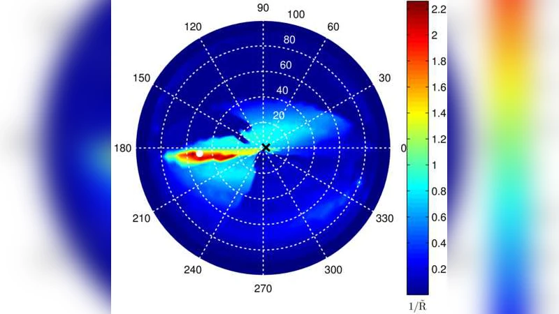
The second critical step in GSR is the determination of the invariant axis. Traditionally, the method projects magnetic‑field data onto a plane perpendicular to a trial axis, computes the transverse pressure Pt(A) curve, and seeks the axis direction that yields two coincident branches (inward and outward spacecraft motion) with minimal residual R. However, the residual map often contains spurious minima caused by short branch lengths or noisy data, leading to ambiguous axis identification. The authors introduce a combined metric ˜R = R · N²/L², where L is the number of data points belonging to each branch and N is the total number of observations. By weighting the residual with branch length, the new “combined residual map” effectively suppresses false minima and highlights the true axis direction. Figures in the paper demonstrate that the filtered map provides a clear, single minimum, whereas the original map shows multiple red zones.

The improved GSR is applied to three case studies. The first event, observed by STEREO‑A on 2008‑11‑07, is a well‑defined MC with low variance magnetic rotation, declining bulk speed, low proton temperature, and low plasma β. The reconstructed axis (θ ≈ 4.3°, φ ≈ 26.1° in RTN coordinates) is nearly perpendicular to the radial solar‑wind flow, consistent with the spacecraft crossing near the flux‑rope apex. The reconstructed magnetic‑potential map shows a clear central maximum and a boundary defined by the minimum of A where the Pt(A) branches still coincide. The second case, a fast ICME recorded by ACE and WIND on 2004‑11‑09, exhibits average speeds >750 km s⁻¹ and two leading shocks. Despite the dynamic environment, the upgraded GSR yields a stable axis (θ ≈ ‑27°, φ ≈ 43° in GSE) for both spacecraft, and the independent reconstructions agree closely, confirming the robustness of the new algorithm under fast‑flow conditions. The third set of events is used to compare the reconstructed transverse‑pressure profiles with the classification scheme of Jian et al. (2006), which groups MCs into three categories based on the shape of Pt(A). The authors find that events classified as “Group 1” (well‑defined pressure peak) tend to have axes nearly perpendicular to the radial direction, whereas “Group 2” (plateau) and “Group 3” (decreasing pressure) show more varied orientations, matching the physical expectation that the spacecraft trajectory relative to the flux‑rope apex influences the observed pressure profile.

The paper also discusses intrinsic limitations of the GSR approach. Because the method assumes a static, two‑dimensional configuration, it cannot fully capture rapid expansion, strong shocks, or significant curvature of the flux rope that occur in fast ICMEs. Moreover, the lack of externally imposed boundary conditions means that the outer parts of the reconstructed map rely on extrapolation of the Pt(A) fit, reducing confidence in the inferred size beyond the region where the two branches overlap. Finally, single‑spacecraft reconstructions are inherently ambiguous; while the authors demonstrate consistency between ACE and WIND when treated separately, a true multi‑spacecraft implementation would benefit from a joint inversion framework.

In summary, the authors present two key methodological enhancements—noise‑robust differentiation and a combined residual‑branch‑length metric—that substantially improve the numerical stability and axis‑identification reliability of Grad‑Shafranov reconstruction. The upgraded technique successfully reproduces the geometry of both typical magnetic clouds and more challenging fast ICMEs, providing more accurate estimates of axis orientation, impact parameter, and cross‑sectional shape. These improvements make GSR a more powerful tool for space‑weather research, particularly for assessing the geoeffectiveness of magnetic clouds and for probing the large‑scale magnetic topology of interplanetary coronal mass ejections.