Sparse recovery with unknown variance: a LASSO-type approach

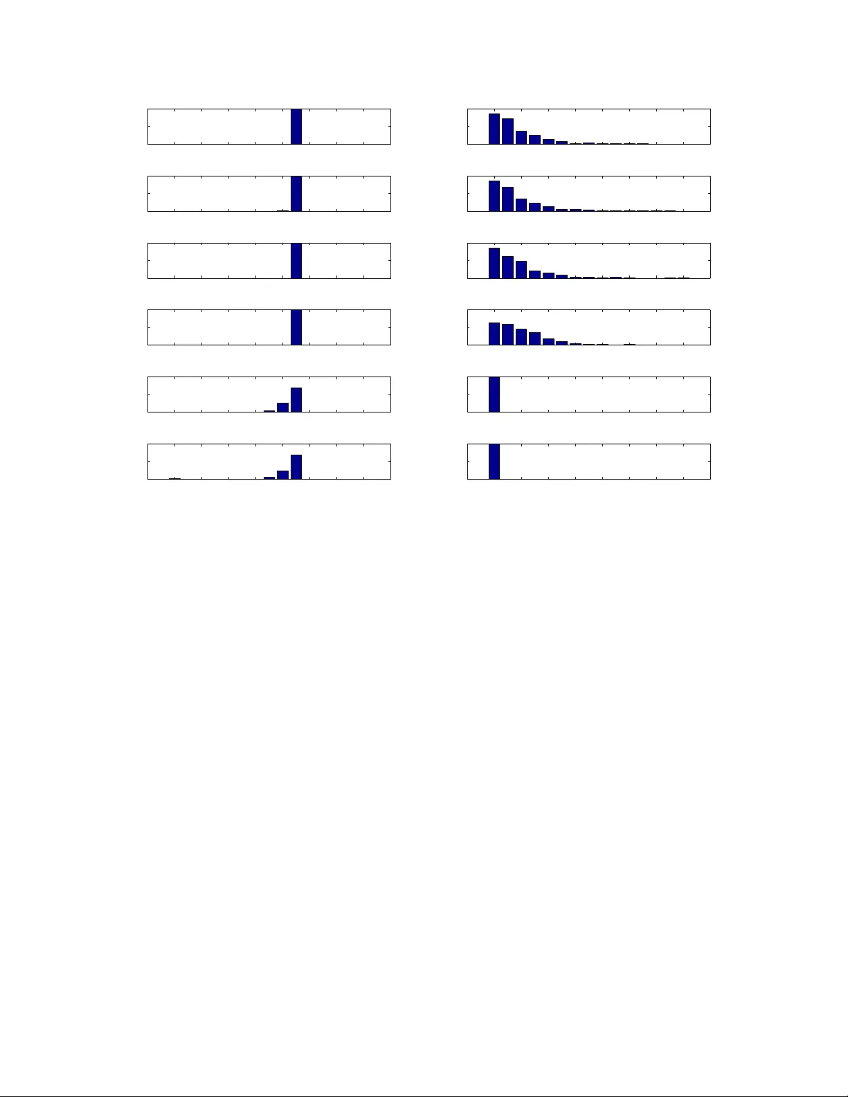
1 Sparse reco v er y with unkno wn v ar iance: a LASSO-type approach Stéphane Chrétien, Sébastien Darses Abstract We addre ss the issue of estimating the regression v ector β in the generic s -sparse line ar mod el y = X β + z , with β ∈ R p , y ∈ R n , z ∼ N (0 , σ 2 I ) and p > n whe n t he v a riance σ 2 is unknown. W e study two L ASSO-type metho ds that jointly esti mate β and the v ar iance. These estimato rs are min imizers of the ℓ 1 penal ized least-square s functional , where the relaxation p arameter i s tuned accordi ng to two different strategies. In the first strategy , the relaxatio n paramete r i s of the order b σ √ log p , where b σ 2 is the empir ical v aria nce. In the second strategy , the relaxati on pa rameter is chosen so as to enforce a tr ade-of f b etween the fidelity and th e penalty terms at op timality . F or bot h estimators, our assumption s are similar to the on es proposed by Cand ès and Plan in An n . Stat. (20 09) , for the case wh ere σ 2 is known. We prov e that ou r estimators en sure e xact recov e ry of the suppo r t and sign patt ern of β with high pro babilit y . We present simulations re sults showing tha t the first estimator enjoys nearly t he same performances in practice a s th e standard LA SSO (known v ar iance case) f or a wide range of the sign al to noise ratio. Our second estimator is shown to outperfor m both in ter ms of f alse detection, when the signal to noise ratio is low . Index T e rms LASSO , sparse regression, ℓ 1 penal ization, hi gh dimensional regression, unknown v ar iance. ✦ 1 I N T R O D U C T I O N 1.1 Pr oblem sta tement The well-known standar d Gaussian linear model r eads y = X β + z , (1.1) wher e X denotes a n × p design matrix , β ∈ R p is an unknown parameter and the components of the erro r z a re assumed i.i.d. with normal distribution N (0 , σ 2 ) . The present paper aims at studying this model in the case where the number of covariates is gr e ater than the number of observations, n < p , and the r e gr ession vector β and the variance σ 2 ar e both unknown. The estimation of the parameters in this case is of course impossible without furt her assump- tions on the regr ession vector β . One such assumption is sparsity , i.e. only a few components of β are dif ferent fro m zero, say s components; β is then said to be s -sparse. There has been a great inter est in the study of this problem recently . R ecovering the support of β has been extensively studied in the context of Compr essed Sensing, a new paradigm for designing observation matri- ces X . I n this framework, it is now a standar d fact that matrices X can be found (e.g. with high pr obability if drawn fr om sub-Gaussian i. i. d distributio ns) such that the number of observations needed to r e cover β exactly is propo rtional to s log ( p/n ) . • S. Chrétien is with the Laboratoire de Mathématiques, UMR 6623, Un iversité de Franche-Comté, 16 route de Gray , 25030 Besancon, France E-mail: stephane.chretien@univ-fcomte.fr • S. Darses is with the LA TP , UMR 6632, Université Aix-Marseille, T echnopôle Château-Gombert, 39 rue Joliot Curie, 1 3453 Marseille Cedex 13, France E-mail: darses@cmi.univ-mrs.fr Manuscript received ?, 201 1; revised ?, 2012. 2 1.2 Existing results in the known v ariance case When the variance is known and positive, two popular techniques to estimate the r egression vector β ar e the Least Absolute Shrinkag e and Selection Operator (LASSO) [33], and t he Dantzig selector [10]. W e r e fe r to [2] for a recent simultaneous analysis of these two methods. The standar d LASSO estimator b β λ of β is defined as b β λ ∈ argmin b ∈ R p 1 2 k y − X b k 2 2 + λ k b k 1 , (1.2) wher e λ > 0 is a r egularization parameter contr olling the sparsity of the estimated coef ficients. Sparse recovery cannot hold without some geometric assumptions on the dictionary (or the design matrix), as recalled in [22] pp. 4–5. The papers [37] and [38] introduced very pe rtinent assumptions for the study of variable selection problem using the LASSO in the finite sample (r esp. asymptotic) contexts. One common assumption for the precise study of the statist ical performance of these estimators is an incoher ence property of the matrix X . This means that the coher ence of X , i.e. the maximum scalar pr oduct of two (normalized) columns of X , is very small. Coherence based conditions appeared first in the context of Basis Pursuit for sparse app r oximation in [13], [17] and [14]. It then had a significant impact on Compress ed Sensing; see [29] and [9]. The recent refer ences [2], [5] and [21] contain interesting assumptions on the coherence in our context of interest, i.e. high dimensional sparse r egr e ssion. For instance, [2] and [5] r equire a bound of the or der p log n/n whereas [21] requir es a bound of the or der 1 /s . The r ece nt paper [8] requir es that the coherence of X is le ss than Cst / log p . Under the additional assumptions that β is sparse and assuming that the support and sign pattern are uniformly distributed, they pr ove that b β has the same support and sign pattern as β with pro bability 1 − p − 1 ((2 π log p ) − 1 / 2 + sp − 1 ) − O ( p − 2 log 2 ) . Notice, as commented on in e.g. [8], that various assumptions in the literatur e, such as the invertibility of the r estricted covariance matrix [37] indexed by the signal’s true support and the Irrepr e se ntable Condition in [38] can be de rived from their incoherence condit ion, althoug h with possibly suboptimal or de rs in certain instances. 1.3 Existing results in the unknown v ariance case The problem of estimating the variance in the sparse regr ession model has been a ddr e ssed in only a few r eferences until now . In [1] the authors analyze in the unknown variance sett ing AIC, BIC and AMDL based est imators, as we l l as estimator s using a mor e general co mplexity penalty . As well known among practitioners, the LASSO pr ocedure, at the price of certain assumptions on X , a voids t he enumeration o f all s ubsets of covariates, an intractable task when the number of covariates is lar ge. This last property mot ivates the theor etical analysis pr ovided in the pr esent paper . In a r e cent work [4], a joint estimation pr ocedure for both the r egr ession vector and the variance is proposed. The authors give a detailed study of the risk under quite general conditions. In [31], it is pr oven in particular that, for the variance estimato r of [4], under a compatibilit y condition introduced i n [36], λ k β k 1 /σ = o (1) if and only if b σ /σ = (1 + o P (1)) , for λ such that P ( λ > a k X t ( Y − X β ) / n k ∞ /σ ) → 1 wher e a > 1 is any constant. The problem of support a nd sign pattern reco very as well as the one of pro viding non-asymptotic results with explicit constants ar e not addressed. 1.4 Our contribution W e study two dif fe rent strategies in the present pa per . 3 1.4.1 Strateg y (A): Plugging in the variance estimator Our work mainly aims at understanding when the result s of [8] extend to the case where σ 2 is unknown. In the case wher e σ 2 is known, it is prov en in [8] that the right order of magnitude for λ is σ √ log p . W e first study the very natural estimator consisting of r e placing σ by b σ = k y − X b β k 2 / √ n in the expressio n of λ . A s is standard in the study of the LASSO, the r egr e ssion vector β ’ s co effi cients have to be sig nificantly larg er than the noise level for exact r ecovery of the support and sign pattern. The main differ ences between the known and the unknown variance cases are summarized in the following table. Known variance Unknown variance: Strategy (A) b β ∈ argmin b ∈ R p k y − X b k 2 2 2 + λ k b k 1 b β λ ∈ argmin b ∈ R p k y − X b k 2 2 2 + λ k b k 1 T une λ to b λ s.t. : b λ = C v ar b σ √ log p λ = cs t σ √ log p with : b σ 2 = k y − X b β b λ k 2 2 n Con ve x problem Non con vex problem Oracle e β Oracle ( e β , e λ ) Conditions holding with high probabilit y Similar conditions Notice that, in this table, b β is defined via b λ and b λ is defined via b β . In other words, b β and b λ jointly satisfy a set of optimality conditions. From a numerical viewpoint, b β and b λ can be computed iteratively using a fixed point-type algorithm; see Section 5.3.1. 1.4.2 Strateg y (B): Enf orcing a trade-off betw een fidelity and penalty Another possible strategy can be used to over come the problem of estimating the r egression vector β and the r e la xation parameter λ when the variance σ 2 is unknown. This strategy consists of pr escribing a trade-of f between the fidelity term and the penalty term. Mor e pr ecisely , we will impos e the constraint b λ k b β k 1 / k y − X b β k 2 2 = C . Enfor cing such a trade-off between fidelity and penalty results in a more complex problem fr om both the statistic al and the computationaly viewpoints. However , since b λ k b β k 1 and k y − X b β k 2 2 ar e, at least approximately , homo geneous functions of σ 2 , using such a criterion allows to bypass the estimation of the variance in a first stage. The variance itself could be estimated in a second stage, using the formula b σ 2 = k y − X b β b λ k 2 2 n . 4 Known variance Unknown variance: Strategy (B) b β ∈ argmin b ∈ R p k y − X b k 2 2 2 + λ k b k 1 b β λ ∈ argmin b ∈ R p k y − X b k 2 2 2 + λ k b k 1 T une λ to b λ s.t. : λ = cst σ √ log p b λ k b β b λ k 1 = C k y − X b β b λ k 2 2 Con ve x problem Non con vex problem Oracle e β Oracle ( e β , e λ ) Conditions holding with Similar conditions high probabilit y + Upp er b ound on k β k 1 1.4.3 Results Our main r e sults ar e Theor em 2.5, for Strategy (A), and Theorem 2.7, for St rategy (B). Both results can be described as follows. Given an arbitrary α > 0 , we pro ve that, for regr ession vectors β satisfying certain natural co nstraints, standard assumptio ns on the number of obs ervations n and the sparsity s imply that our modified LASSO pr ocedur e s fail to identify the support and the signs of β with probabilit y at most of the order p − α . These results ar e non-asymptotic and all our constants are e xplicit. The co her ence assumption on the design matrix made in this paper is r eadily checkable. Many other currently used assumptions in the literatur e are based on concentratio n pro perties of the extr eme sing ular values of a ll or most extracted submatrices of X with bounded number of columns. Y e t, some other are based on the concentration of the singular values of the covariance matrix with r espect to t he covariate’s unde rlying distribution. All such criteria are diffic ult or impossible to check in practice as opposed to the coher ence propert y . W e neither make any uncheckable assumption on the variance σ 2 . The only unverifiable as- sumptions used in the pr esent work ar e on the magnitude of the nonzer o r egr e ssion coef ficients. As in [8], the set of regr essors β which are corr ectly estimated is constrained by imposing that the magnitude of all nonzero components of β should be gr eater than the noise level. Mor eover , for Strategy (B), our analysis requir es the additional assumption that the components of β should not be too large either , the upper bound being in particular a function of C . This r esult suggests that Strategy (B) is pertinent in low SNR situations only . Simulation experiments at the end of this paper confirm the usefulness of Strategy (B) in the low SNR setting. 1.5 Plan of the paper The LASSO est imator , the main r esults Theorem 2.5 and Theorem 2.7, together with the assump- tions used thr oughout the paper are pr e sented in Section 2. The pr oof of Theor e m 2.5 is given in Section 3 and the pro of of Theorem 2.7 in Section 4. The p roofs of certain technical intermediate r esults are gathered in the Appendix. 5 1.6 Notations 1.6.1 Genera lities When E ⊂ { 1 , . . . , N } , we denote by | E | the cardinal of E . For I ⊂ { 1 , . . . , p } and x a vector in R p , we set x I = ( x i ) i ∈ I ∈ R | I | . The usual scalar pro duct is denoted by h· , ·i . The notat ions for the norms on vectors and matrices are also standard: for any vector x = ( x i ) ∈ R N , k x k 2 2 = X 1 ≤ i ≤ N x 2 i ; k x k 1 = X 1 ≤ i ≤ N | x i | ; k x k ∞ = sup 1 ≤ i ≤ N | x i | . For any matrix A ∈ R d 1 × d 2 , we denote by A t its transpose. The set of symmetric r eal matrices in R n × n is denoted by S n . W e denote by k A k the operator norm of A . The maximum (r esp. minimum) singular value of A is de noted by σ max ( A ) (r esp. σ min ( A ) ). Recall that σ max ( A ) = k A k and, if A is invertible, σ min ( A ) − 1 = k A − 1 k . W e use the Loewner o r dering on sy mmetric real matrices: if A ∈ S n , 0  A is equivalent to saying that A is positive semi-definite, and A  B stands for 0  B − A . The notations N ( µ, σ 2 ) (resp. χ 2 ( ν ) and B ( ν ) ) st ands for the normal distribution on the real line with mean µ and variance σ 2 (r esp. the Chi-square distribution with ν degr e es of freedom and the Bernoulli distribution with parameter ν ). 1.6.2 Specific notations related to the design matrix X and the estimators For I ⊂ { 1 , . . . , p } , a nd a matrix X , we denote by X I the submatrix whose columns are indexed by I . W e denote the range of X I by V I and the orthogonal pro jection onto V I by P V I . The coher ence µ ( X ) of a matrix X whose columns ar e unit-norm is defined by µ ( X ) = max 1 ≤ i 6 = j ≤ p |h X i , X j i| . (1.3) As in [34], we consider the ’hollow-gram’ matrix H and the selector matrix R = diag ( δ ) : H = X t X − Id (1.4) R = diag( δ ) , (1.5) wher e δ is a vector of length p whose components are i.i.d. random variables following the Bernoulli distributio n B ( s/p ) . In a similar fashion, we define R s = diag( δ ( s ) ) wher e δ ( s ) is a ran- dom vecto r of length p , uniformly distributed on the set of all vectors with exactly s co mponents equal to 1 and p − s component s equal to 0. The support of b β is always denoted by b T . 2 T H E M O D I FI E D L A S S O E S T I M ATO R S In this section, we p resent the main result s on the e stimators given by Strategy (A ) a nd Strategy (B), and we discuss the underlying assumptions. Practical computability of these estimators will be st udied in Section 5. I n particular "tuning λ to b λ " is achieved by finding a zer o of a function o f λ numerically . W e will show in Section 5 that these zero finding problems are comput ationally very easy to solve. For any a rbitrary value of α > 0 , Theorem 2.5 (r esp. Theor e m 2.7), pr oposes a set of co nditions under which exact reco very of the support and sign pattern of β holds with pr obability at le ast 1 − O ( p − α ) for Strategy (A) (r esp. for Strategy (B)). As will be shortly seen, the ma gnitude of the nonzero coefficients of β has to satisfy certain constraints : as in [8], one will r equire for both Strategies that t he nonzero components of β ar e not too small (in fact, slightly above the noise level). In the case of Strateg y (B), we will mor e over requir e that the nonzer o components of β are not too lar ge. Altho ugh this upper 6 bound assumption may seem to argue in disfavor of St rategy (B), computational experiments will later show that this Strategy has much nicer empirical performance whe n t he signal to noise ratio is small. The same comput ational experiments will also demonstrate that Strategy (A) performs almost as well as a standard L A SSO which would know the variance. 2.1 Definition of the estimators T o de fine our estimators, we first need to work with matrices ensuring that the ma p λ 7→ b β λ , wher e b β λ is given by (1.2), is well defined and enjoys special propert ies, such as continuity . Definition 2.1: The matrix X is said to satisfy the Generic Condition if   h x j , X I ( X t I X I ) − 1 δ I i   < 1 , ∀ δ ∈ {− 1 , 1 } p , ∀ I ⊂ { 1 , . . . , p } s.t. X I non singular and ∀ j 6∈ I . (2.6) As fr om now , we a lwa ys work under the Generic C ondition. W e will use the following r esult about uniqueness of the LASSO estimator . Proposition 2. 2 ([15]): Assume that X satisfies the Generic Condition. Then, for all y ∈ R n , and for all λ ∈ R + , Pr oblem (1.2) has a unique solution b β λ and its support b T λ is such that X b T λ is non singular . The following pro perty is pr oven in Append ix C.2.1: Lemma 2.3: Let the Generic Condition hold. Then, almost sur e ly , the map  (0 , + ∞ ) − → R p λ 7− → b β λ is bounded and continuous. Mor eover , its ℓ 1 -norm is non-incr ea sing. 2.1.1 Strateg y A The estimator of strategy A is defined as b β := b β b λ wher e b λ verifies the implicit equation b λ 2 = C v ar    y − X b β b λ    2 2 n log p. (2.7) The estimators ( b β , b λ ) being implicitly defined, it is not clear , at that point, that they exist. W e will see in the sequel that a suitable choic e of C v ar will ensur e the existence of the e stimator s (under the above mentioned assumptions on X ). The uniqueness follows by showing that the map Γ A : R + → R + given by Γ A ( λ ) := n log p λ 2 k y − X b T λ b β b T λ k 2 2 , is incr e asing, which is pr oven in Appe nd ix C.2. Strategy A simply reduces to finding the value b λ A such that Γ A ( b λ A ) = C v ar . A precise range of inter est for C v ar will be given in Theorem 2.5 below . Mor eover , using the existence a nd uniqueness r esult, one can use a fixed point scheme to find b λ . This scheme is discussed in Section 5.3.1. Remark 2.4: Recall that in the known variance case, it is often assumed that λ 2 = C v ar σ 2 log p, (2.8) 7 for some positive constant C v ar ; see e.g. in [8]. In comparison, Strategy (A) enforces the c hoice (2.7). T h is is the empiric al analog to (2.8). However , as will appear later in the pro of of Theorem 2.5, instead of bei ng an absolute constant, C v ar will have to depend on n , p and k X k 2 as follows C v ar ≍ n p k X k 2 . In the c ase of an i.i.d. Gaussian random de sign matrix, k X k 2 is of the order p/n with hi gh proba bility . Thus C v ar can be basically seen as a constant in the Gaussian setting. 2.1.2 Strateg y B The estimator of strategy B is defined as b β := b β b λ wher e b λ verifies the implicit equation b λ k b β λ k 1 = C    y − X b β b λ    2 2 . (2.9) Again, the estimators ( b β , b λ ) ar e implicitly defined and their existence has to be pro ven. Compared to Strategy A, one specificity of Strategy B is that for any value of C > 0 , existence and uniquene ss of the estimators is gar anteed, with no other assumptions than the Generic Condition. Indeed, we show her e (cf Lemma C.3 in the Append ix) that the map Γ B given by Γ B ( λ ) = λ k b β λ k 1 k y − X b β λ k 2 2 , λ > 0 , (2.10) is increasing, continuous and Γ B ((0 , + ∞ )) = (0 , + ∞ ) . Thus, ther e exists a unique value b λ B > 0 such that Γ B ( b λ B ) = C . Similarly as for Strategy A, a fixed point scheme will be discussed in Section 5. 2.2 Main results 2.2.1 Prelimina r y remarks The main ide a behind the analysis of L A SSO-ty pe methods is the following. First, the ℓ 1 penalty pr omotes sparsity of the est imator b β . Since b β is sparse, we may r estrict the st udy to the subvector b β b T of b β , resp. the submatrix X b T of X , whose components, resp. columns , are in d e xed by b T . T a king this idea a litt le further , since b T is supposed to e stimate the true support T of car d ina lity s , t he first kind of r e sult one may ask for is a pr oof that X T is far fr om singular for every possible T . U nfortunat ely , proving such a strong property with the right or der in the upp e r bound on s , based on incoherence only , seems to be impossible. The idea proposed by C andès and Plan in [8] to overc ome this problem is to assume that T is random and then pr ove that non-singularity occurs with high pr obability , i.e. for most supports. Based on this model, the method first consists of pr oving that X T satisfies, for 0 < r < 1 , 1 − r ≤ σ min ( X T ) ≤ σ max ( X T ) ≤ 1 + r , (2.11) with high probability . The pr oof of this propert y in [8] is based on the Non-Commutat ive Kahane- Kintchine inequalities. I n the pr esent paper , we instead use a resu lt of [11] based on a recent version of the Non-Commutative Che rnof f ine quality pr oposed by T r opp [35], in order to obtain better estimates for the involved constants. The most intuitive conditions to prov e (2.11) are: (i) T is a random support with uniform distribution on ind e x sets with car dinal s ; (ii) s is suf ficiently small; (iii) X is sufficiently incoher e nt. 8 The main part o f the analysis cons ists of pr oving that the least-squar es oracle estimator , which knows the support ahe ad of time, satisfies the opt imality conditions of the LASSO estimator with high probability . This will pr ove that the LASSO automatic ally detects the r ight suppo rt and sign pattern. The proof s of these results highly dep e nd on the q ua si-isometry co ndition (2.11) a nd similar propert ies obtained with the same techniques as for (2.11). W e also need the sign pattern of β to be uniformly distributed and jointly inde pendent of the support of T . This assumption was alr eady invoked in [8]. 2.2.2 Assumptions and main results The first so-called Coherence conditio n deals with the minimum angle between the columns of X . Assumptions 2.1: (Range a nd Coherence condition for X ) The matrix X has unit ℓ 2 -norm columns, is full rank and its coher e nce verifies µ ( X ) ≤ C µ log p , for some numerical constant C µ > 0 . Assumptions 2.2: (Generic sparse model [8]) 1) The support T of β is random and has uniform distribut i on among all index subsets of { 1 , . . . , n } with cardinal s , 2) Given T , the sign pattern of β T is random with uniform distribution over {− 1 , +1 } s , and jointly independent of the support. The last condition concerns the magnitude of the nonzero regr ession coefficients β j , j ∈ T . Let α > 0 , r ∈ (0 , 1 2 ] and κ = 4 √ 1 + α . (2.12) Let us now define H n,s 0 ,p α,r = 4 √ n + √ 2 α log p √ s 0 1 − r √ 1 + r . (2.13) Let us intr oduce the function ℓ α ( x ) = xe − 4 α/x , x > 0 . Since ℓ α ((0 , + ∞ )) = (0 , + ∞ ) , the following constant C ◦ := C ◦ ( α, r ) is well defined: ℓ α ( C ◦ ) = 10 e 1 + r (1 − r ) 2 κ 2 > 0 . (2.14) It will appear in the number n of observations (explaining the index ’ ◦ ’). W e can now de fine the range assumption for the coef ficients of β for Strategy (A). Assumptions 2.3: (Range condition for β : Strategy (A)) The unknown vector β verifies min j ∈ T | β j | ≥ H n,s 0 ,p α,r σ . (2.15) Our main r esults show that the estimators b β d e fined by either Strategy (A) or Strategy (B) r ecovers the support and sign pattern of β exactly with pr obability of the order 1 − O ( p − α ) using 9 similar bounds on the coher ence and the sparsity as in [8]. As fr om now , let us choose r ∈ (0 , 1 2 ] and set: C spar = r 2 (1 + α ) e 2 (2.16) C µ = r 1 + α . (2.17) Theorem 2.5: Let α > 0 and p ≥ e 8 /α . Let Assumption 2.1 hold wit h C µ given above. Let Assumptions 2.2 and 2.3 hold with s ≤ s 0 := p log p C spar k X k 2 (2.18) n ≥ s ( C ◦ log p + 1 ) . (2.19) Then the pro bability that the estimator b β defined by Strategy (A) with C v ar ∈  (1 − r ) 2 20(1 + r ) C spar n p k X k 2 ; (1 − r ) 2 2(1 + r ) C spar n p k X k 2  , (2.20 ) exactly r ecovers the support and sign pattern of β is greater than 1 − 2 28 /p α . Remark 2.6: The choiCe of the constant 20 is unessential and the reader can che ck for himself which range is r e levant for his own specific application. W e now turn to Strateg y (B). Let us define for C > 0 , L n,s,p α,r,C = max  2 √ 1 + 2 C C √ 1 − r √ n − s + √ 2 α log p √ s , 2 √ s + √ 2 α log p √ 1 − r √ s  (2.21) M n,s,p α,r,C = n − s √ log p 1 3 κC p π ( n − s ) p α ! 4 n − s . (2.22) Let us state the corr esponding range assumption for the coef ficients of β . Assumptions 2.4: (Range condition for β : Strategy (B)) The unknown vector β verifies min i ∈ T | β j | ≥ L n,s,p α,r,C σ , (2.23) k β k 1 ≤ M n,s,p α,r,C σ . (2.24) Theorem 2.7: Let α > 0 , p ≥ e 8 /α and set c ◦ = (6 κ ) 2 e 1 − r . Choose C > 0 . Let Assumptions 2.1, 2.2 and 2.4 hold with s ≤ p log p C spar k X k 2 , (2.25) n ≥ c ◦ (1 + 2 C ) s log p + s. (2.26) Then the probabilit y that the estimator b β defined by Strategy (B) exactly recovers the support and sign pattern of β is greater than 1 − 22 9 /p α . 10 2.3 Impor tant comments 2.3.1 About X The normalized Gaussian example is instructive. First, when X is obtained fro m a random matrix with i.i. d . st andard Gaussian random entries by normalizing the columns, the coher e nce is of the order p log p/n (See be low for a short pr oof). Ther efore, taking n of the or der of log 3 p is suf ficient for satisfying the Incoherence Assumption 2.1. Second, it is also well known that k X k 2 is of the or de r p/n , see e.g. [30]. This suggests in particular that the upper bound (2.25) on the number s of nonzer o components of β may be understood in the Gaussian setting as s ≤ p log p C spar k X k 2 = O  n log p  . This or de r of magnitude might be also valid for much mor e general random designs. Notice that the estimate p log p/n of the coher ence for i.i.d. Gaussian matrices with normalized columns easily follows from the Paul Levy concentration of measur e phenomenon on the spher e and the union bound: Since, due to normalization, each column is Haar distributed on the unit spher e, rotatio nal invariance implies that the scalar produc t of two column vectors X j and X j ′ satisfies P ( |h X j , X j ′ i| ≥ u ) = P ( |h X j , X j ′ i| ≥ u | X j ′ ) ≤ 2 exp  − cn u 2  , for some const ant c , by the well known co ncentration of measur e phenomenon on the unit spher e. Thus, the union bound gives P  max 1 ≤ j 0 . T o make a fair comparison, let us also choose α = 1 . 5 > 2 log 2 and r = 1 / 2 . W e obtain: C spar ≃ 1 . 4 10 − 2 , C µ = 0 . 2 . 3 P R O O F O F T H E O R E M 2 . 5 The pr oof is divided into several steps. The main two steps ar e as follows. First, we prov ide the description and consequences of the optimality conditions for the standard LASSO estimator as a function of λ . Second, we pr ove that these optimality conditions are satisfied by a simple and natural oracle estimator . 12 3.1 Enf orc ing the in ver tibility assumption W e r e call the ba sic result we proved in [11] regar d ing the invertibility of random submatrices via the Non-commutative Chernoff I nequality . Theorem 3.1: Let r ∈ (0 , 1) , α ≥ 1 . Let X be a full-rank n × p matrix and s be positive integer , such that µ ( X ) ≤ r 2(1 + α ) log p s ≤ r 2 4(1 + α ) e 2 p k X k 2 log p . Let T ⊂ { 1 , . . . , p } be a set with cardinality s , chosen randomly fro m the uniform distribution. Then the following bound holds: P  k X t T X T − Id s k ≥ r  ≤ 216 p α . (3.28) By Theor e m 3.1, we have (1 + r ) − 1 ≤ k  X t T X T  − 1 k ≤ (1 − r ) − 1 (3.29) (1 − r ) 1 / 2 ≤ k X T k ≤ (1 + r ) 1 / 2 (3.30) with probability gr eater than 1 − 216 p − α . Thus, thr oughout this section, we will assume that (3.29) and (3.30) hold, i.e. we will r educe all events consider e d to their intersection with the event that (3.29) and (3.30) ar e satisfied. 3.2 The orac le estimator f or b β and b λ W e now discuss the next step of the proof of Theorem 2.5, which consists of studying some sort of oracle estimators for β which enjoys the p roperty of knowing the support T of β ahead of time. For a given e λ , one might like to consider the following oracle for b β : β ∈ argmax b ∈B − 1 2 k y − X b k 2 2 − e λ k b k 1 , (3.31) wher e B = { b ∈ R p , supp( b ) = T , sgn( b ) = sgn( β T ) } . However , it is not so easy to derive a closed form expr ession for β . Therefo r e, it might be mor e inter esting to consider instead the following oracle: e β ∈ argmax b ∈ R p , supp( b )= T − 1 2 k y − X b k 2 2 − e λ sgn( β T ) t b. (3.32) Indeed, e β satisfies X t T  y − X T e β T  − e λ sgn( β T ) = 0 , and we obtain that e β is given by e β T =  X t T X T  − 1  X t T y − e λ sgn( β T )  . (3.33) 13 This formula is the same as in the pr oof of Th. 1.3 in [8], but here, e λ is a variable. Now let us r e call that in the known variance case, Candès and Plan assume that λ 2 = C v ar σ 2 log p, (3.34) for some positive constant C v ar . It is then relevant to see k our oracle e λ as: e λ 2 = C v ar k y − X T e β T k 2 2 n log p. (3.35) Replacing e β by its value (3.33), we obtain C v ar k y − X T  X t T X T  − 1  X t T y − e λ sgn( β T )  k 2 2 = n log p e λ 2 . Thus, C v ar k P V ⊥ T y + e λX T  X t T X T  − 1 sgn( β T ) k 2 2 = n log p e λ 2 , and using the orthogo nality r e l a tions, we obtain C v ar k P V ⊥ T y k 2 2 + e λ 2 C v ar k X T  X t T X T  − 1 sgn( β T ) k 2 2 = n log p e λ 2 , which is equivalent to e λ 2 = k P V ⊥ T z k 2 2 n C v ar log p − k X T ( X t T X T ) − 1 sgn( β T ) k 2 2 (3.36) W e he nce forth work with this de finition of e λ . Notice that e λ is well defined whenever C v ar ≤ n k X T ( X t T X T ) − 1 sgn( β T ) k 2 2 log p . (3.37) The choice of C v ar will be done in the next section. 3.3 Study of the orac le e λ In this section, we provide a confidence interval for e λ . In particular , the first subsection shows that e λ is well defined. 3.3.1 Bound s on k X T ( X t T X T ) − 1 sgn( β T ) k 2 2 Using the lower bound on σ min ( X T ) and the upper bound on σ max ( X T ) g iven by (3.29) and (3.30), we have, with high pro bability: 1 − r (1 + r ) 2 s ≤ k X T ( X t T X T ) − 1 sgn( β T ) k 2 2 ≤ 1 + r (1 − r ) 2 s. (3.38) W e write the choice of C v ar made in (2.20) as 1 20 (1 − r ) 2 1 + r n s 0 log p ≤ C v ar ≤ 1 2 (1 − r ) 2 1 + r n s 0 log p , (3.39) wher e s 0 is the maximum sparsity allowed in Inequality (2.18), namely , s 0 = p log p C spar k X k 2 . In particular , the condition (3.37) is satisfied which garantees that e λ is indeed well defined. 14 3.3.2 Bound s on k P V ⊥ T z k 2 Using some well known pr operties o f the χ 2 distribution recalled in Lemma B.1 in the Appe nd ix, we obtain that P  k P V ⊥ T ( z ) k 2 /σ ≥ √ n − s + √ 2 t  ≤ exp( − t ) (3.40) and P  k P V ⊥ T ( z ) k 2 2 /σ 2 ≤ u ( n − s )  ≤ 2 p π ( n − s ) ( u e/ 2) n − s 4 . (3.41) T une u such that the r .h.s. of (3.41) equals 2 /p α , i.e. u = 2 e p π ( n − s ) p α ! 4 / ( n − s ) . Thus, we obtain that k P V ⊥ T z k 2 2 σ 2 ≤ √ n − s + r 2 log( p α 2 ) ! 2 ≤  √ n − s + p 2 α log p  2 (3.42) and k P V ⊥ T z k 2 2 σ 2 ≥ 2( n − s ) e p π ( n − s ) p α ! 4 / ( n − s ) (3.43) with pr obability gr eater than or equal to 1 − 2 p − α . 3.3.3 Bound s on ˜ λ Lemma 3.2: The following bounds hold: e λ ≤ σ 1 − r √ 1 + r √ n − s + √ 2 α log p √ s 0 (3.44) e λ ≥ κ σ p log p. (3.45) Proo f: Recall that 0 ≤ s ≤ s 0 . Fr om (3.39), we have C v ar ≤ 1 2 (1 − r ) 2 1 + r n s 0 log p . W e then obtain, by virtue of (3.36) and the upper bound in (3.38), e λ 2 ≤ k P V ⊥ T z k 2 2 2 s 0 1+ r (1 − r ) 2 − k X T ( X t T X T ) − 1 sgn( β T ) k 2 2 ≤ k P V ⊥ T z k 2 2 2 s 0 1+ r (1 − r ) 2 − s 0 1+ r (1 − r ) 2 . Using the bound (3.42), we deduce (3.44). On the other hand, the bound (3.43) and n C v ar log p ≤ 20 1 + r (1 − r ) 2 s 0 , 15 yield e λ 2 ≥ 2( n − s ) e  π ( n − s ) p 2 α  2 / ( n − s ) σ 2 20 1+ r (1 − r ) 2 s 0 . Fr om (2.19), we know that n verifies n − s s 0 ≥ n − s 0 s 0 ≥ C ◦ log p. (3.46) Thus, noting that ( π ( n − s )) 2 / ( n − s ) ≥ 1 , e λ 2 ≥ (1 − r ) 2 10 e (1 + r ) p − 4 α/ ( n − s ) C ◦ σ 2 log p. W riting p − 4 α/ ( n − s ) = e − 4 α log p/ ( n − s ) and, using (3.46) again, log p n − s ≤ log p n − s 0 ≤ 1 s 0 C ◦ ≤ 1 C ◦ , we obtain p − 4 α/ ( n − s ) ≥ e − 4 α/C ◦ . Ther efor e , e λ 2 ≥ (1 − r ) 2 10 e (1 + r ) e − 4 α/C ◦ C ◦ σ 2 log p. (3.47) Let us r ecall that the constant C ◦ has been pr ecisely chosen to satisfy ℓ α ( C ◦ ) = C ◦ e − 4 α/C ◦ = 10 e 1 + r (1 − r ) 2 κ 2 . As a conclusion, we have just pro ved (3.45). 3.4 Candès and Plan’ s condi tions T o obt ain the exact recovery of the support and sign patterns of β , we will need similar bounds as the ones in [8, Section 3.5]. Namely , (i) k ( X t T X T ) − 1 X t T z k ∞ ≤ κ σ √ log p (ii) k ( X t T X T ) − 1 sgn( β T ) k ∞ ≤ 3 (iii) k X t T c X T ( X t T X T ) − 1 sgn( β T ) k ∞ ≤ 1 4 (iv) k X t T c (Id − X T ( X t T X T ) − 1 X t T ) z k ∞ ≤ κ σ √ log p (v) k X t T X T − Id s k ≤ r . When r = 1 2 , these conditions were proven to hold with high probability in [8] based on pr evious results due t o T r opp [34]. Most of t he pro ofs that these conditions hold wit h high pr obability are the same as in [8] up to some slight impro vements of the constants. Proposition 3. 3 : The bounds (i-iv) hold with pr obability at least 1 − 10 /p α . Condition (v) holds with pr obability at least 1 − 216 /p α . Proo f: See Section A in the Appen d ix. 16 3.5 Last step of the proof W e now conclude the pr oof using the strategy announced in the beginning of this section: (i) W e pro ve that the proxies e β and e λ satisfy the optimality conditions (C.89) and (C. 9 0), fro m which we deduce that b β = e β and b λ = e λ . (ii) Since the pr oxy e β ha s the right support and sign patt erns, we co nclude that b β e xactly r ecovers these features as well. 3.5.1 e β and β hav e the same suppor t and sign patter n First, it is clear that e β and β have the same support. Next, we must pr ove that e β has the same sign pattern as β . Use Pr oposition 3.3 to obtain k e β T − β T k ∞ ≤ k ( X t T X T ) − 1 X t T z k ∞ + e λ k ( X t T X T ) − 1 sgn( β T ) k ∞ ≤ κ σ p log p + 3 e λ. Using the lower bound (3.45), and the expressio n of κ , we obtain k e β T − β T k ∞ ≤ 4 e λ. (3.48) A sufficient condition t o guarantee that the sign patt ern is r ecovered is that this last upper bound be lower than the minimum absolute value of non-zero component s of β , i.e. 4 e λ ≤ min j ∈ T | β j | . (3.49) Using the upper bound on e λ in (3.44), this is achieved in particular when 4 σ √ n − s + p 2 α log( p ) √ s 0 1 − r √ 1 + r ≤ min j ∈ T | β j | , which is implied by Assumption 2.4. 3.5.2 e β and e λ satisfy the optimal ity conditions Using the lower bou nd (3.45) on e λ , the pr oof of the fact e β and e λ satisfy the optimality conditions is exactly the same as in [8, Section 3.5]. W e r epeat the ar gument for the sake of completeness. On one hand, by constr uction, we clearly ha ve X t T ( y − X e β ) = − e λ sgn( β T ) . Since e β and β have the same sign pattern, we a ctually ha ve: X t T ( y − X e β ) = − e λ sgn( e β T ) . On the other hand, k X t T c ( y − X e β ) k ∞ = k X t T c P V ⊥ ( z ) + e λ X t T c X T ( X t T X T ) − 1 sgn( β T ) k ∞ ≤ k X t T c P V ⊥ ( z ) k ∞ + e λ k X t T c X T ( X t T X T ) − 1 sgn( β T ) k ∞ ≤ κ σ p log p + 1 4 e λ (3.50) ≤ 3 4 e λ < e λ. Hence, the two parts of the subgradient conditions (C.89-C . 9 0) ar e satisfied by e β and e λ , which means that e β = b β e λ . (3.51) 17 In other wor ds, e β corr esponds t o the solution of pro blem (1.2) with the penaliz a tion λ = e λ . Mor eover , e λ bas been determined so that it verifies (3.35) e λ 2 = C v ar k y − X T e β T k 2 2 n log p, i.e., plugging (3.51), e λ 2 = C v ar k y − X T ( b β e λ ) T k 2 2 n log p. Ther efor e , e λ is a solution of Eq . (2.7). By virtue of uniqueness proved in Ap p e ndix C.3, we deduce that b β = e β b λ = e λ. 3.5.3 Conclusion of the proof The two pr eceding sub-sect ions pr ove that b β has same support and sign pattern as β . This occurs when (3.2 9) and (3.30) (both implied by the invertibility condition (v) in Sec. 3.4), Candè s and Plan’s conditions (i-iv) in Sec. 3.4 and the bound on k P V ⊥ T z k 2 in Sec. 3.3.2 are satisfied simultaneously . Ther efor e, this occurs with pro bability at least 1 − 216 + 10 + 2 p α , as announced. 4 P R O O F O F T H E O R E M 2 . 7 As in the proof of Theor e m 2.5, the quasi-isometry pr operty (3.29) and (3.30), and C a ndès and Plan’s conditions of Section 3.4 will be assumed. Notice also that the results of Section C.1 are still valid with the assumption of Theor em 2.7. 4.1 The orac le estimator As in the case of Section 3.2, the oracle for β is given by e β T =  X t T X T  − 1  X t T y − e λ sgn( β T )  . (4.52) W e now seek e λ verifying 1 2 k y − X T e β T k 2 2 = C e λ sgn( β T ) t e β T . (4.53) Replacing e β by its value (3.33), we obtain 1 2 k y − X T  X t T X T  − 1  X t T y − e λ sgn( β T )  k 2 2 = C e λ sgn( β T ) t   X t T X T  − 1  X t T y − e λ sgn( β T )  . Thus, 1 2 k P V ⊥ T y + e λX T  X t T X T  − 1 sgn( β T ) k 2 2 = − C e λ 2 h sgn( β T ) ,  X t T X T  − 1 sgn( β T ) i + C e λ sgn( β T ) t  X t T X T  − 1 X t T y . 18 Using the orthogo nality r e lations, we then obtain 1 2 k P V ⊥ T y k 2 2 + e λ 2 2 k X T  X t T X T  − 1 sgn( β T ) k 2 2 = C e λ sgn( β T ) t  X t T X T  − 1 X t T y − C e λ 2 h sgn( β T ) ,  X t T X T  − 1 sgn( β T ) i , which is equivalent to  1 2 + C  e λ 2 k  X t T X T  − 1 2 sgn( β T ) k 2 2 − C e λ sgn( β T ) t  X t T X T  − 1 X t T y + 1 2 k P V ⊥ T z k 2 2 = 0 . (4.54) The ro ots of the quadratic equation are e λ = C sgn( β T ) t ( X t T X T ) − 1 X t T y ± √ ∆ (1 + 2 C ) k ( X t T X T ) − 1 2 sgn( β T ) k 2 2 , (4.55) wher e ∆ =  C sgn( β T ) t  X t T X T  − 1 X t T y  2 − (1 + 2 C ) k  X t T X T  − 1 2 sgn( β T ) k 2 2 k P V ⊥ T z k 2 2 . 4.2 Study of the orac le ˜ λ Following the same strategy as for Strategy (A), we now pro vide a confidence interval for ˜ λ . 4.2.1 Premilina ries W e have sgn( β T ) t  X t T X T  − 1 X t T y = sgn( β T ) t  X t T X T  − 1 X t T ( X T β + z ) = sgn( β T ) t β + sgn( β T ) t  X t T X T  − 1 X t T z = k β k 1 + h X T  X t T X T  − 1 sgn( β T ) , P V T z + P V ⊥ T z i . Hence, sgn( β T ) t  X t T X T  − 1 X t T y = k β k 1 + h X T  X t T X T  − 1 sgn( β T ) , P V T z i . (4.56) Note that the Cauchy-Schwarz inequality yields    h X T  X t T X T  − 1 sgn( β T ) , P V T z i    ≤ k  X t T X T  − 1 2 sgn( β T ) k 2 k P V T z k 2 . (4.57) 4.2.2 Bound on k P V T z k 2 Using some well known pr operties o f the χ 2 distribution recalled in Lemma B.1 in the Appe nd ix, we obtain P  k P V T ( z ) k 2 /σ ≥ √ s + √ 2 t  ≤ exp( − t ) . (4.58) T une t such that e − t = 2 p − α , i.e. t = log( p α / 2) . Hence, P  k P V T ( z ) k 2 /σ ≥ √ s + p 2 log ( p α / 2)  ≤ p − α . (4.59) 19 4.2.3 P ositivit y of ∆ W e begin with the study of sgn( β T ) t ( X t T X T ) − 1 X t T y and k ( X t T X T ) − 1 2 sgn( β T ) k 2 2 k P V ⊥ T z k 2 2 , two key quantities in the analysis. W e first study sgn( β T ) t ( X t T X T ) − 1 X t T y . By (3.29), we have k  X t T X T  − 1 2 sgn( β T ) k 2 ≤ r s 1 − r . (4.60) Thus, using (4.59), (4.57) and the lower bound (2.23) fr om Assumption 2.4 on the non-zero components of β , we can write    h X T  X t T X T  − 1 sgn( β T ) , P V T z i    ≤ σ √ s √ 1 − r  √ s + p 2 α log p  ≤ 1 2 k β k 1 . Ther efor e , fr om (4.56) we deduce that 1 2 k β k 1 ≤ sgn ( β T ) t  X t T X T  − 1 X t T y ≤ 3 2 k β k 1 . (4.61) Second, we study k ( X t T X T ) − 1 2 sgn( β T ) k 2 2 k P V ⊥ T z k 2 2 . W e have k  X t T X T  − 1 2 sgn( β T ) k 2 k P V ⊥ T z k 2 ≤ σ r s 1 − r  √ n − s + p 2 α log p  . Thus ∆ ≥ C 2 4 k β k 2 1 − σ 2 (1 + 2 C ) s 1 − r  √ n − s + p 2 α log p  2 (4.62) ≥ C 2 4 s 2 min 1 ≤ j ≤ p | β j | 2 − σ 2 (1 + 2 C ) s 1 − r  √ n − s + p 2 α log p  2 (4.63) and Assumption 2.4 shows that ∆ > 0 , which ensures that e λ is well defined. 4.2.4 Bound s on ˜ λ First, let us write √ ∆ =  C sgn( β T ) t  X t T X T  − 1 X t T y  × v u u u t 1 − (1 + 2 C ) k ( X t T X T ) − 1 2 sgn( β T ) k 2 2 k P V ⊥ T z k 2 2  C sgn( β T ) t ( X t T X T ) − 1 X t T y  2 . On one hand, due to √ 1 − δ ≤ 1 − δ 2 on (0 , 1) , we obtain √ ∆ ≤  C sgn( β T ) t  X t T X T  − 1 X t T y  − (1 + 2 C ) k ( X t T X T ) − 1 2 sgn( β T ) k 2 2 k P V ⊥ T z k 2 2 2 C sgn( β T ) t ( X t T X T ) − 1 X t T y . 20 Combining this last equation with (4.55), we obtain that e λ ≥ k P V ⊥ T z k 2 2 2 C sgn( β T ) t ( X t T X T ) − 1 X t T y . (4.64) On the other hand, we also have √ 1 − δ ≥ 1 − δ on (0 , 1 ) . Thus we can write √ ∆ ≥  C sgn( β T ) t  X t T X T  − 1 X t T y  − (1 + 2 C ) k ( X t T X T ) − 1 2 sgn( β T ) k 2 2 k P V ⊥ T z k 2 2 C sgn( β T ) t ( X t T X T ) − 1 X t T y and combining this last equation with (4.55) and the previo us upper bound, we thus obtain e λ ≤ k P V ⊥ T z k 2 2 C sgn( β T ) t ( X t T X T ) − 1 X t T y . Using (4.61), we finally get k P V ⊥ T z k 2 2 3 C k β k 1 ≤ e λ ≤ 2 k P V ⊥ T z k 2 2 C k β k 1 . (4.65) Combining this last equation with (3.43), we obtain: σ 2 ( n − s )  √ π ( n − s ) p α  4 n − s 3 C k β k 1 ≤ e λ ≤ 2 σ 2  √ n − s + √ 2 α log p  2 C k β k 1 . (4.66) Using Assumption 2.4 and (2.22), we thus obtain e λ ≥ κ σ p log p. (4.67) 4.3 Last step of the proof 4.3.1 e β and β hav e the same suppor t and sign patter n As in the case of Strategy (A) it is clear that ˜ β and β have the same support. Let us now verify that they have the same sign pattern. As in Section 3.5.1 and based on (4.67), we obtain k e β T − β T k ∞ ≤ 4 e λ, exactly as for Strategy (A). U sing the upper bound on e λ in the right hand side of (4.66), we thus need 8  √ n − s + √ 2 α log p  2 C ≤ min j ∈ T | β j | k β k 1 σ 2 to garantee that e β T and β T have the same sign pattern. In view of this inequality , and since k β k 1 ≥ s min j ∈ T | β j | , an even str onger sufficient conditio n is 8  √ n − s + √ 2 α log p  2 C s ≤ min j ∈ T | β j | 2 σ 2 . Noting that 2 √ 2 √ C ≤ 2 √ 1+2 C C √ 1 − r , we conclude that this condition is also implied by Assumption 2.4. 21 4.3.2 e β and e λ satisfy the optimal ity conditions The pro of is exactly the same as in Section 3.5.2 after replacing (3.45) by (4.67). 4.3.3 Conclusion of the proof The two pr e ce d ing sub-sections prove that b β has same support and sign pa ttern as β . This occurs under the same conditions as those mentioned in the conclusion of the pr oof of The or em 2.5, Sec. 3.5.3, plus the bound on k P V T z k 2 in Sec. 4.2.2. Hence, this occurs with pr obability at least 1 − 216 + 10 + 2 + 1 p α , as announced. 4.4 Epilogue: Nonempty range for k β k 1 W e need to ensure that the range of admissible values for β is suffi ciently large. The intuition says that this can be achieved by allowing suf ficiently larg e values of n . In other wo r ds, we would like to know the additional constraints on the various parameters ensuring s L n,s,p α,r,C < M n,s,p α,r,θ,C . It then suf fices to know when the following inequalities are satisfied: m α,r,C s √ n − s + √ 2 α log p √ s ≤ n − s √ log p p π ( n − s ) p α ! 4 n − s (4.68) wher e m α,r,C = 6 κ √ 1 + 2 C √ 1 − r . First, notice that under the condition n − s ≥ 8 α s log p ≥ 8 α log p, (4.69) we have log  √ π ( n − s ) p α  4 n − s = 4 ( n − s )  1 2 (log( π ) + log ( n − s )) − α lo g p  ≥ − 1 2 , and then e − 1 / 2 ≤ p π ( n − s ) p α ! 4 n − s . Ther efor e , since we also have √ 2 α log p ≤ √ n − s , (4.68) is fulfilled if 2 m α,r,C √ s √ n − s ≤ e − 1 / 2 n − s √ log p , i.e. n − s ≥ 4 e m 2 α,r,C s log p. This explains the constraint (2.26) with the constant c ◦ := 4 e m 2 α,r,C > 8 α . 22 5 A L G O R I T H M S A N D S I M U L AT I O N S R E S U LT S In this section, we p r opose one iterative algorithm for Strategies (A) and (B) and we study their practical performance via Monte Carlo experiments. W e performed Mo nte Carlo experiments in the following sett ing. W e too k p = 600 , n = 75 and s = 9 and we ran 500 experiments with σ 2 = 1 and the coefficients of β were randomly drawn independently as B times a Bernoulli ± 1 random variable plus a n independent center ed Gaussian perturbation with variance one. 5.1 Preliminaries Our algorithms will be well defined under the assumption that for each positive value of the r elaxation parameter , the value b β λ of the r egr e ssion vector is unique and the trajectory of b β λ is continuous and piecewise af fine. This pro perty is well known under various assumptions on the design matrix X . It is a basic prer equisite for the theory behind Least Angle Re gr ession and Homotopy methods. W e refer the reader to [26] and [16] for information on these problems. See also [15] for a r ecent account on the study of b β λ as a function of λ under generic condit ions on the design matrix. The subgradient conditions for the LASSO imply that X t b T λ ( y − X b T λ b β b T λ ) = λ sgn( b β b T λ ) . (5.70) wher e X b T λ is non-singular , and we ob tain the well known fact that, for a ny λ > 0 such that b β λ 6 = 0 , b β b T λ = ( X t b T λ X b T λ ) − 1  X t b T λ y − λ sgn  b β b T λ  . (5.71) The following r esult is straightforw ar d but useful. Lemma 5.1: (Nontriviality of the estimator) Let Σ be the set Σ =  ( S, δ ); S ⊂ { 1 , . . . , p } , δ ∈ {− 1 , 1 } | S | , | S | ≤ n, σ min ( X S ) > 0  . (5.72) The inequality inf ( S,δ ) ∈ Σ   ( X t S X S ) − 1 ( X t S y − λ δ )   1 > 0 (5.73) holds with pro bability one. Proo f: This is an immediate consequence of the Gaussian distribution of z . 5.2 The standar d LASSO with known v ariance 5.2.1 Simul ations results: high SNR W ith the choice B = 40 , in all of the 500 experiments, we found that the support was exactly r ecover ed . 5.2.2 Simul ations results: low SNR Figur e 5.2.2 below shows the histogram of the number of pr operly recover ed components (left column) and the number of false components (r ight column) fo r the L A SSO estimator with known variance and λ = 2 σ √ 2 log p . 23 −2 0 2 4 6 8 10 12 14 16 0 0.2 0.4 Number of recovered components, mean =6.614, stdev=1.2776 Frequency −2 0 2 4 6 8 10 12 14 16 0 0.5 1 Number of recovered components, mean =8.372, stdev=0.75016 Frequency −2 0 2 4 6 8 10 12 14 16 0 0.5 1 Number of recovered components, mean =9, stdev=0 Frequency −2 0 2 4 6 8 10 12 14 16 0 0.5 1 Number of recovered components, mean =8.996, stdev=0.089443 Frequency −2 0 2 4 6 8 10 12 14 16 0 0.2 0.4 Number of incorrectly detected components, mean =2.536, stdev=1.8186 Frequency −2 0 2 4 6 8 10 12 14 16 0 0.2 0.4 Number of incorrectly detected components, mean =3.39, stdev=2.4646 Frequency −2 0 2 4 6 8 10 12 14 16 0 0.1 0.2 Number of incorrectly detected components, mean =3.62, stdev=2.9511 Frequency −2 0 2 4 6 8 10 12 14 16 0 0.1 0.2 Number of incorrectly detected components, mean =4.042, stdev=3.6164 Frequency Figure 1. Histogr am of the numb er of pro perly recov ered components (le ft column) an d the numb er of f alse compo nents (right column) for the LASSO estimator with known variance and λ = 2 σ √ 2 log p f or coeff . mean le vel B = 1 , 2 , 5 , 10 (from top to bottom) 5.3 Strategy (A) 5.3.1 The algorithm As was discussed in Section 2.1.1, finding the estimator ( b β , b λ ) in Strategy A is equivalent to solving the equation Γ A ( λ ) = C v ar . Since the function Γ A is increasing (see Appendix C.2), ther e is a number of Newton-type methods which can be used to solve this equation very ef ficiently and globally , i.e. without a ny condition on the initial iterate λ (0) ; see e.g. [28]. I nstead of such a refined me thod, we propo se below a simpler fixed point iteration which was observed to work very well in practice. Notice that the first step of the fixed point iteration pr ocedur e is similar to the correct ion of the standar d estimator of σ proposed by [31]. 5.3.2 Simul ations results: high SNR As for the case of the standard LASSO with known variance of Section 5.2.1 we found that, for B = 40 , the support was exactly recov ered in all of the 500 experiments. 24 Algorithm 1 Fixed point iterations for the LASSO with unknown variance Input λ (0) , l = 1 and ε > 0 while | λ ( l +1) − λ ( l ) | ≥ ε do Compute b β λ ( l ) as a solution of the LASSO pr oblem b β λ ( l ) ∈ argmin b ∈ R p 1 2 k y − X b k 2 2 + λ ( l ) k b k 1 (5.74) Set λ ( l +1) = C v ar √ n k y − X b β ( l ) λ ( l ) k 2 l ← l + 1 end while Set b λ ( L ) = λ ( L ) , b β ( L ) = b β λ ( L ) and b σ ( L ) = 1 √ n k y − X b β ( l ) λ ( l ) k 2 . Output b β ( L ) , b σ ( L ) and b λ ( L ) . 5.3.3 Simul ations results: low SNR W e pe rformed Mont e Carlo experiments in the same setting as for the LA SSO in Section 5.2.2. In real situations where the level of magnitude of the regr ession coeffi cients may not be much higher than the noise level, one observ es that false positives often occur for the LA SSO estimator with known variance. A s seen from these r esults, the LASSO estimator where the variance is estimated using the pe nalty b λ = 2 b σ √ 2 log p performs at least as well as the standard LASSO estimator to which the tr ue variance is available. The estimator b σ of the standard deviation is a slightly biased as shown in Figur e 5.3.3. 5.4 Strategy (B) 5.4.1 The algorithm Basic computations show that the derivative of Γ with respect to λ is given by d Γ B dλ ( λ ) = −k b β b T λ k 1 − λ k ( X t b T λ X b T λ ) − 1 / 2 sign  b β b T λ  k 2 2 k y − X b β λ k 2 2 on e a ch ˚ I k , wher e ˚ I k , is a maximal open interval on which the support of b β λ is const ant, for k ∈ K and ∪ k ∈K I k is a connected interval of [0 , + ∞ ) . See for instance [12, Section 4]. In order to compute the LASSO estimators ( b β , b λ ) satis fying the penalty vs. fidelity tradeoff constraint, we need to find b λ such that Γ B ( b λ ) = C . Since Γ is strictly decreasing by Lemma C.3, this task is not diffi cult to p e rform. A simple Newton-Raphson pr ocedur e for solving this equation is summarized in Algorithm 5.4.1 below . 5.4.2 Simul ations results: high SNR As for the case of the standard LASSO with known variance of Section 5.2.1 we found that, for B = 40 , the support was exactly recov ered in all of the 100 experiments. 5.4.3 Simul ations results: low SNR W e pe rformed Mont e Carlo experiments in the same setting as for the LA SSO in Section 5.2.2. Figur e 5. 4 .3 below shows the histogram of the number of properly r ecover e d components (left column) and the number of false components (right column) for the LASSO estimator with unknown variance and the pe nalty vs. fidelity tradeoff constr aint for the values C = . 01 , . 1 , . 5 . 25 −2 0 2 4 6 8 10 12 14 16 0 0.2 0.4 Number of recovered components, mean =6.564, stdev=1.2904 Frequency −2 0 2 4 6 8 10 12 14 16 0 0.5 1 Number of recovered components, mean =8.36, stdev=0.75335 Frequency −2 0 2 4 6 8 10 12 14 16 0 0.5 1 Number of recovered components, mean =9, stdev=0 Frequency −2 0 2 4 6 8 10 12 14 16 0 0.5 1 Number of recovered components, mean =8.996, stdev=0.089443 Frequency −2 0 2 4 6 8 10 12 14 16 0 0.2 0.4 Number of incorrectly detected components, mean =2.008, stdev=1.6448 Frequency −2 0 2 4 6 8 10 12 14 16 0 0.2 0.4 Number of incorrectly detected components, mean =2.782, stdev=2.1381 Frequency −2 0 2 4 6 8 10 12 14 16 0 0.2 0.4 Number of incorrectly detected components, mean =2.988, stdev=2.7755 Frequency −2 0 2 4 6 8 10 12 14 16 0 0.1 0.2 Number of incorrectly detected components, mean =3.376, stdev=3.4973 Frequency Figure 2. Histogr am of the number of properly recover ed components (left column) and the number of f alse components (right col umn) f or t he LA SSO e stimator with un known v ar iance usin g Strategy (A) and b λ = 2 b σ √ 2 log p f or coeff . mean le vel B = 1 , 2 , 5 , 10 (from top t o b ottom). The instances wher e Newton’s iterations did not converge wer e simply discar de d although implementing a line search or a tr ust r egion strategy could easily have p roduced a corr ect r esult at the price of increasing the computational time for the Monte Carlo simulations study . The number of well recov er ed components of β is always e qual to the true value 9 as C incr e ases for all values of C . On the other hand, the number of false positives increases with C . Our estimator with penalty vs. fide lity tradeoff constraint is seen to have quite better perfor - mances than the standar d LASSO and LASSO with e stimated variance of the previous section with respect to the number of false posit ives; compar e Figur e 5.4.3 wit h the second row of Figur e 5.2.2 or Figur e 5.3. 3 . This was the main objective for proposing this strategy and the presented simulations show encouraging evidence of its r obust behavior in the low SNR case. The low dependency on C is a property which might be well app reciated in practice when neither the signal nor the noise levels are p r ecisely known ahe ad of time. 5.5 Comments The simulations resu lts confirmed the theoretical findings that, in the high SNR case, S trategy (A) and Strategy (B) perform a s well, without knowing the variance ahe ad of time, as the standar d LASSO which uses the tr ue value of the variance. Althoug h the results ar e pr esented for a particular set of parameters, this behavior was observed more generally for a large number of numerical experiments with differ ent parameter configurations, for which the standard LASSO 26 −0.5 0 0.5 1 1.5 2 2.5 0 0.2 0.4 −0.5 0 0.5 1 1.5 2 2.5 0 0.2 0.4 −0.5 0 0.5 1 1.5 2 2.5 0 0.2 0.4 −0.5 0 0.5 1 1.5 2 2.5 0 0.2 0.4 Figure 3. Histogr am of b σ for the LASSO estimator with unkno wn variance using Strate gy (A) and b λ = 2 b σ √ 2 log p f or coeff . mean le vel B = 1 , 2 , 5 , 10 (from top to bottom). Algorithm 2 Newton’s method for the LASSO with penalty vs. fidelity tradeof f constraint Input λ (0) , l = 1 and ε > 0 while | λ ( l +1) − λ ( l ) | ≥ ε do Compute b β λ ( l ) as a solution of the LASSO pr oblem b β λ ( l ) ∈ argmin b ∈ R p 1 2 k y − X b k 2 2 + λ ( l ) k b k 1 (5.75) Set λ ( l +1) = λ ( l ) − d Γ B dλ ( λ ( l ) ) − 1 Γ( λ ( l ) ) l ← l + 1 end while Set b λ ( L ) = λ ( L ) , b β ( L ) = b β λ ( L ) and let b σ ( L ) 2 be given by b σ ( L ) 2 = k y − X b β ( L ) k 2 2 + 2 b λ ( L ) k b β ( L ) k 1 n (5.76) Output b β ( L ) , b σ ( L ) 2 and b λ ( L ) . exactly recovers the true support and sign pa ttern. I n the low SNR setting, the standard L A SSO and Strategy (A) perform poorly in the sense that many false components ar e selected. The Monte Carlo experiments show that Strategy (B) is more ro bust in the low SNR setting, in the sense that the e stimated support contains much le ss false components. Surprisingly , this phenomenon was observed over a wide range of values for the constant C . In other words, the dep e ndence of Strategy (B)’s performance on C appeared as rather unessential for the recovery problem in the low SNR setting. A s a pr eliminary practical conclusion, Strategy (A ) appeared to be more 27 −2 0 2 4 6 8 10 12 14 16 0 0.5 1 Number of recovered components, mean =8.998, stdev=0.044721 Frequency −2 0 2 4 6 8 10 12 14 16 0 0.5 1 Number of recovered components, mean =8.994, stdev=0.077304 Frequency −2 0 2 4 6 8 10 12 14 16 0 0.5 1 Number of recovered components, mean =9, stdev=0 Frequency −2 0 2 4 6 8 10 12 14 16 0 0.5 1 Number of recovered components, mean =9, stdev=0 Frequency −2 0 2 4 6 8 10 12 14 16 0 0.5 1 Number of recovered components, mean =8.524, stdev=1.1663 Frequency −2 0 2 4 6 8 10 12 14 16 0 0.5 1 Number of recovered components, mean =8.474, stdev=1.3465 Frequency −2 0 2 4 6 8 10 12 14 16 0 0.2 0.4 Number of incorrectly detected components, mean =1.6076, stdev=2.0281 Frequency −2 0 2 4 6 8 10 12 14 16 0 0.2 0.4 Number of incorrectly detected components, mean =1.7726, stdev=2.3703 Frequency −2 0 2 4 6 8 10 12 14 16 0 0.2 0.4 Number of incorrectly detected components, mean =1.6687, stdev=2.0299 Frequency −2 0 2 4 6 8 10 12 14 16 0 0.2 0.4 Number of incorrectly detected components, mean =2.0703, stdev=2.1879 Frequency −2 0 2 4 6 8 10 12 14 16 0 0.5 1 Number of incorrectly detected components, mean =0.875, stdev=2.4749 Frequency −2 0 2 4 6 8 10 12 14 16 0 0.5 1 Number of incorrectly detected components, mean =0, stdev=0 Frequency Figure 4. Histogr am of the number of properly recover ed components (left column) and the number of f alse components (right col umn) f or t he LA SSO e stimator with un known v ar iance usin g Strategy (B) f or C = 0 . 01 , . 01 , 0 . 5 , 1 , 5 , 10 (from top to bottom) with le vel B = 5 . suitable for the high SNR sett ing and Strategy (B) mor e suitable for the low SNR sett ing. In practice, the choice of C in Strategy B could be based on standar d model selection proc edures (AIC, BI C, Foster and Georg e, etc) for comparing the obtained supports over a large range of possible values. The limited number of possible support s occur ring in practice as C varies makes this comparison numerically tractable. Another inter e sting question is the one of the convergence of the algorithms pr oposed for Strategies (A) and (B). Fr om the practical viewpoint, let us report that converg ence was observed except in rar e cases d uring the Monte Ca rlo experiments. However , we decided not to pursue their theor etical ana lysis here, since more r obust methods enjoying global conver gence have been pr oposed in the literature during the last twenty years. W e r e fer the interested r e ader to e.g. [28] for a globally converg ent damped Newton method. Such methods are however more delicate to implement and the algorithms pr oposed in the present paper seem to be a goo d choice to start with in most practical experiments. Finally , there r emains the question of choosing between Strategy A and Strategy B on a given practical pro blem. One reaso nable way to proc eed might simply be as follows: compar e the supports obtained via both methods, using a standard model selection pr ocedure such as BIC, AIC, Foster and Geor ge’s criterion, etc. 28 A P P E N D I X A P R O O F O F P R O P O S I T I O N 3 . 3 First, let us r e call a technical result we obtained in [11]: Lemma A.1: The following bound holds: P ( k RH k 1 → 2 ≥ v ) ≤ p  e s p k X k 2 v 2  v 2 /µ ( X ) 2 , (A.77) pr ovided that e s p k X k 2 v 2 ≤ 1 . Let us intr oduce the events: E = {k X t T X T − Id k ≤ r } B =  k RH k 1 → 2 ≤ c √ log p  . The proofs that Conditions ( i ) and ( ii ) hold with high probabilit y are trivial modifications of the ones given in [8] up to the constants. The proofs that Conditions ( iii ) and ( iv ) hold with high probabilit y can be performed using the following by-pr oduct ine quality fr om our Lemma A.1: P ( B c ) ≤ p exp  c 2 C 2 µ log  e C spar c 2  log p  , (A.78) instead of using [8, Lemma 3.5] and [8, Lemma 3.6]. Here, we take c 2 ≥ max( e 2 C spar ; (1 + α ) C µ ) , (A.79) so that P ( B c ) ≤ 1 p α . (A.80) All the pr oofs are mor eover based on the simple inequality P ( A ) = P ( A ∩ E ∩ B ) + P ( A ∩ ( E c ∪ B c )) ≤ E [ P ( A | R ) 1 E ∩ B ] + P ( E c ) + P ( B c ) , and the bound, for a given vector W : P ( |h W, X i| > t ) ≤ 2 e − t 2 / (2 k W k 2 2 ) . ( A.81) This last bound holds tr ue for sub-Gaussian random vectors with independent co mponents having Bernoulli or standar d Gaussian distribution, for instance. A.1 Condition ( i ) Here, let W i be the i th row of ( X t T X T ) − 1 X t T . Since h W i , z i ∼ N (0 , k W i k 2 2 ) , we have from (A.81 ) and the union bound: P  max i ∈ T |h W i , z i| > t  ≤ 2 s e − t 2 / (2 max i k W i k 2 2 ) . Note that on E : max i ∈ T k W i k 2 ≤ k ( X t T X T ) − 1 k k X t T k ≤ √ 1 + r 1 − r . (A.82) 29 One then obtains P  k ( X t T X T ) − 1 X t T z k ∞ ≤ σ κ p log p  ≥ 1 − 2 p α , whenever κ ≥ p 2(1 + α )(1 + r ) 1 − r . (A.83) A.2 Condition ( ii ) Let us show that the estimate ( ii ) holds with high pr obability . This is an actual consequence of our Lemma A.1. First, as in [8] p.2171 and Lemma 3.3 p.2166, we write the inequality k ( X t T X T ) − 1 sgn( β T ) k ∞ ≤ 1 + max i ∈ T |h W i , sgn( β T ) i| , wher e W i is the i th ro w or column of ( X t T X T ) − 1 − Id . Set A =  max i ∈ J |h W i , sgn( β T ) i| ≥ 2  . Hoef fding’s inequality yields: P ( A| R ) ≤ 2 | J | exp   − 2 2 2 max i ∈ J k W i k 2 2   . (A.84) As in [8] p.2171 and p.2172, we write k W i k 2 ≤ k RH Re i k 2 1 − r . Thus on E : k W i k 2 ≤ k RH R k 1 → 2 1 − r ≤ k RH k 1 → 2 1 − r . Recall that P ( B c ) ≤ 1 p α since c satisfies (A.79). Mor e over E [ P ( A | R ) 1 E ∩ B ] ≤ 1 p α holds tr ue if c 2 ≤ 2(1 − r ) 1 + α . W e can e asily check that this last condition is compatible with (A.79) and C µ = r 1 + α C spar = r 2 (1 + α ) e 2 , whenever r ∈ (0 , 1 / 2 ) . Ther efore, when r ∈ (0 , 1 / 2) , the event k ( X t T X T ) − 1 sgn( β T ) k ∞ ≤ 1 + 2 = 3 holds with pro bability at least 1 − 3 p α . 30 A.3 Condition ( iii ) Here, W i = ( X t T X T ) − 1 X t T X i . Notice that on E ∩ B : max i ∈ T c k W i k 2 ≤ c (1 − r ) √ log p . (A.85) Using (A.80) again and the same pr evious arg uments, we obtain P  k X t T c X T ( X t T X T ) − 1 sgn( β T ) k ∞ ≤ 1 4  ≥ 1 − 3 p α . A.4 Condition ( iv ) If one now sets W i as the i th r ow of Id − X T ( X t T X T ) − 1 X t T and note that on E for any i ∈ T : k W i k 2 ≤ k X i k 2 = 1 , (A.86) then: P  k X t T c  I − X T ( X t T X T ) − 1 X t T  z k ∞ ≤ σ κ p log p  ≥ 1 − 2 p α , whenever κ ≥ p 2(1 + α ) . (A .87) A.5 Choosing κ The parameter κ has to satisfy (A.83) and (A.87). Since r ∈ (0 , 1 2 ] , one has √ 2(1+ r ) 1 − r ≤ 2 √ 3 ≈ 3 . 4 . Thus we simply chose κ = 4 √ 1 + α , which is Eq. (2.12). A P P E N D I X B S O M E P R O P E R T I E S O F T H E χ 2 D I S T R I B U T I O N W e recall the following useful bounds for the χ 2 ( ν ) distribution of degree of freedom ν Lemma B.1: The following bounds hold: P  χ ( ν ) ≥ √ ν + √ 2 t  ≤ exp( − t ) P  χ ( ν ) ≤ √ uν  ≤ 2 √ π ν ( u e/ 2) ν 4 . Proo f: For the first statement, see e.g. [24]. For the second statement, recall that P  χ 2 ( ν ) ≤ uν  = Z u ν 2 0 t ν 2 − 1 e − t Γ( ν 2 ) dt = Z u ν 2 0 t ν 2 − 1 − α t α e − t Γ( ν 2 ) dt. Since max t ∈ R + t α e − t = ( α/e ) α and is attained at t = α , we obtain that P  χ 2 ( ν ) ≤ uν  ≤ ( α/e ) α Γ( ν 2 ) Z u ν 2 0 t ν 2 − 1 − α dt = ( α/e ) α ( ν 2 − α )Γ( ν 2 )  u ν 2  ν 2 − α . 31 T a ke for instance α = ν 4 and obtain P  χ 2 ( ν ) ≤ uν  = ( ν / 4 e ) ν 4 ν 4 Γ( ν 2 )  u ν 2  ν 4 . (B.88) On the other hand, we have Γ( z ) ≥ √ 2 π z z − 1 2 e z and then, ( ν / 4 e ) ν 4 ν 4 Γ( ν 2 ) ≤ r 2 π ( e/ 2) ν 4  ν 2  − ν 4 p ν 2 . Hence, P  χ 2 ( ν ) ≤ uν  ≤ r 2 π ( u e/ 2) ν 4 p ν 2 = 2 √ π ν ( u e/ 2) ν 4 , as desired. A P P E N D I X C P R O P E R T I E S O F T H E S T A N DA R D L A S S O C.1 Reminders on the LASS O subgradient conditions In [18] Section III, it is proven that a necessary and suf ficient optimality condition in (1.2) is the two following conditions: X t T ( y − X b β λ ) = λ sgn( β T ) (C.89) k X t T c ( y − X b β λ ) k ∞ ≤ λ. (C.90) Mor eover , if k X t T c ( y − X b β λ ) k ∞ < λ , then pr oblem (1.2) admits a unique solutio n. Let us also r e call (see [15] and [12]) that the support b T λ ⊂ { 1 , . . . , p } of b β λ verifies | b T λ | ≤ n. (C.91) C.2 General properties of λ 7→ b β λ Recall that b β λ is the standar d LASSO estimator of β parametrized by λ , The following notations will be useful. Define L as the cost function: L : ( (0 , + ∞ ) × R p − → R + ( λ, b ) 7− → 1 2 k y − X b k 2 2 + λ k b k 1 , (C.92) and for all λ > 0 , θ ( λ ) = inf b ∈ R p L ( λ, b ) . Lemma C.1: Let the Generic Condition hold. Then, the function θ is concave and non-decreasing . Proo f: Since θ is the infimum of a set of affine functions of the variable λ , it is concave. Mor eover , we have θ ( λ ) = L ( λ, b β λ ) , 32 wher e, by Pro position 2.2 , b β is the unique solution of (2). Using the filling pr operty [20, C hapter XII], we obtain that ∂ θ ( λ ) is the singleton {k b β λ k 1 } . Thus, θ is differ entiable and its derivative at λ is given by θ ′ ( λ ) = k b β λ k 1 . Mor eover , this last express ion shows that θ is nondecreasing. C .2.1 Proof of Lemma 2.3 (i) k b β λ k 1 is non-incr easi ng – The fact that λ 7− → k b β λ k 1 is non-incr easing is a n immediate conse- quence of the concavity of θ . (ii) Boundedness – Notice that using (5.71), we obtain that k b β λ k 1 ≤ max ( S,δ ) ∈ Σ   ( X t S X S ) − 1 ( X t S y − λ δ )   1 . Thus, λ 7− → b β λ is bounded on any interval of the form (0 , M ] , with M ∈ (0 , + ∞ ) . Moreover , since its ℓ 1 -norm is non-incr ea sing, it is bounded on (0 , ∞ ) . (iii) Cont inuity – Assume for contradictio n that λ 7− → b β λ is not continuous at some λ ◦ > 0 . Using boundedness, we can const ruct two sequences conver ging towar ds b β + λ ◦ and b β − λ ◦ r espectively with b β + λ ◦ 6 = b β − λ ◦ . Since L ( λ ◦ , · ) is continuous, both limits are optimal solutions of the p roblem argmin b ∈ R p L ( λ ◦ , b ) , (C.93) hence contradict ing the uniquen e ss. C .2.2 P ar titioning (0 , + ∞ ) into good inter vals The continuity of λ 7→ b β λ implies that the interval (0 , + ∞ ) can be partitioned into subintervals of the type I k = ( λ k , λ k +1 ] , with (i) λ 0 = 0 and λ k ∈ (0 , + ∞ ] for k > 0 , (ii) the support and sign pattern of b β λ ar e constant on each ˚ I k . Notice further that due to Step 1.a , b T λ 6 = ∅ on at least I 0 . Let K be the nonempty set K = n k ∈ N , ∀ λ ∈ ˚ I k , b β λ 6 = 0 o . On any interval I k , k ∈ K , uniqueness of b β implies that the e xpr ession (5.71) for b β b T λ holds. Multiplying (5.71) on the left by sgn  b β b T λ  t , we obtain k b β λ k 1 = sgn  b β b T λ  t ( X t b T λ X b T λ ) − 1 X t T y − λ sgn  b β b T λ  t ( X t b T λ X b T λ ) − 1 sgn  b β b T λ  . Thus d k b β λ k 1 dλ ( λ ) = − sgn  b β b T λ  t ( X t b T λ X b T λ ) − 1 sgn  b β b T λ  , on (0 , + ∞ ) . Thus, the definition of Σ , we obtain that d k b β λ k 1 dλ ( λ ) ≤ − inf ( S,δ ) ∈ Σ δ t ( X t b T λ X b T λ ) − 2 δ < 0 (C.9 4) on each ˚ I k , k ∈ K and d k b β λ k 1 dλ ( λ ) = 0 33 on each ˚ I k , k 6∈ K , i.e. on each ˚ I k such that k b β b T λ k 1 = 0 for all λ in I k , if any such I k exists. Since λ 7− → k b β λ k 1 is continuous on (0 , ∞ ) , (C.94) implies that: (i) ther e exists τ ∈ (0 , + ∞ ) , such that b β τ = 0 (as an easy consequence of the Fundamental Theor em of Calculus and a contradiction). (ii) b β λ = 0 for all λ ≥ τ . Hence ∪ k ∈K I k is a connected bounded interval. C .2.3 | b T λ | = n fo r λ sufficien tly small. Let ( λ k ) k ∈ N be any positive sequence conver ging to 0 . Let β ∗ be any cluster point of the s equence ( b β λ k ) k ∈ N (this sequence is easily seen to be bounded under various standar d assumptions; see e.g. [12, Lemma 3.5] for a proo f). Fix ε > 0 and b ∈ R p . For all k ∈ N , we have L ( λ k , b β λ k ) ≤ L ( λ k , b ) , (C.95) wher e L is defined by (C.92 ). Sinc e L ( λ k , · ) is continuous, we can also write for k sufficient ly lar ge: L ( λ k , β ∗ ) ≤ L ( λ k , b β λ k ) + ε. Hence, L ( λ k , β ∗ ) ≤ L ( λ k , b ) + ε . Letting λ k → 0 , we obtain 1 2 k y − X β ∗ k 2 2 ≤ 1 2 k y − X b k 2 2 + ε, and thus, 1 2 k y − X β ∗ k 2 2 ≤ inf b ∈ R p 1 2 k y − X b k 2 2 . (C.96) Since range( X ) = R n , (C.96) implies k y − X β ∗ k 2 2 = 0 , and then lim λ ↓ 0 k y − X b β λ k 2 2 = 0 . (C.97) Notice further that { b ∈ R p , | supp( b ) | < n } is a finite union of subs paces o f R p , each with dimension n − 1 . Thus, m := inf { b ∈ R p ; | supp( b ) | 0 , with pr obability one. Ther efor e for λ suf ficiently small, (C.97) implies k y − X b β λ k 2 2 < m , fro m which we deduce that | b T λ | = n since one ha s | b T λ | ≤ n (cf Remind er C .1). C .2.4 T he map λ 7→ k y − X b β λ k 2 is increasing on (0 , τ ] Using (5.71), we obtain y − X b β λ = P V ⊥ b T λ ( y ) − λX b T λ ( X t b T λ X b T λ ) − 1 sgn  b β b T λ  , which implies that k y − X b β λ k 2 2 =     P V ⊥ b T λ ( y )     2 2 − 2 λ h P V ⊥ b T λ ( y ) , X b T λ ( X t b T λ X b T λ ) − 1 sgn  b β b T λ  i + λ 2 sgn  b β b T λ  t ( X t b T λ X b T λ ) − 1 sgn  b β b T λ  34 and thus, by the definition of P V ⊥ b T λ ( y ) , k y − X b β λ k 2 2 =     P V ⊥ b T λ ( y )     2 2 + λ 2 sgn  b β b T λ  t ( X t b T λ X b T λ ) − 1 sgn  b β b T λ  . (C.98) Fr om (C.98), since ( X t b T λ X b T λ ) − 1 is definite, we obtain that λ 7→ k y − X b β λ k 2 is increasing on e ach ˚ I k , and thus on (0 , τ ] by using that λ 7→ k y − X b β λ k 2 is continuous on (0 , τ ] . C.3 Study of Γ A Lemma C.2: Γ A is incr e asing on (0 , τ ] and lim λ → + ∞ Γ A ( λ ) = + ∞ . Proo f: Due to Step 3, and the definition of τ , the set of values λ > 0 such that k y − X b β λ k 2 > 0 is nonempty . Let λ inf denote its infimum value. T ake λ ∈ ˚ I k for some k such that λ ≥ λ inf . In particular , λ 6 = 0 . The n, Γ A ( λ ) = s 1 λ 2     P V ⊥ b T λ ( y )     2 2 + sgn  b β b T λ  t ( X t b T λ X b T λ ) − 1 sgn  b β b T λ  , (C.99) and we d e duce that Γ A is incr e asing on ˚ I k . By continuity , we ha ve that Γ A is incr e asing on ( λ inf , τ ] . Once λ > τ , k y − X b β λ k 2 2 = k y k 2 2 and Γ A ( λ ) = sλ 2 / k y k 2 2 . Thus, lim λ → + ∞ Γ A ( λ ) = + ∞ as desir ed. The fact that Γ A is incr easing proves t hat the eq uation Γ A ( λ ) = C v ar admits at most one solution. C.4 Study of Γ B Recall that Γ B ( λ ) = λ k b β λ k 1 k y − X b β λ k 2 2 . (C.100) W e will use repeatedly that b β λ is unique for all λ > 0 and that the trajectory λ 7→ b β λ is continuous under the Generic Condition, see [15]. Lemma C.3: Under the Generic Position Assumption of [15], the fu nction Γ B defined by (C.100) almost sur ely satisfies lim λ ↓ 0 Γ B ( λ ) = + ∞ . (C.101) Mor eover , a lmost sur ely , there exists τ > 0 such that Γ B is decr easing on the interval (0 , τ ] with Γ B ( τ ) = 0 , while k y − X b β λ k 2 is incr e asing on (0 , τ ] . Proo f: Let us first show that lim λ ↓ 0 Γ B ( λ ) = + ∞ . Let λ 0 > 0 be sufficiently small so that for all λ ≤ λ 0 , | b T λ | = n . Such a λ 0 exists due to Step 1.a . Hence, since X b T λ is nonsingular: P V T λ = Id n . (C.102) 35 Thus, using (5.71), we obtain y − X b β λ = − λX b T λ ( X t b T λ X b T λ ) − 1 sgn  b β b T λ  , (C.103) which implies that k y − X b β λ k 2 2 = λ 2 k ( X t b T λ X b T λ ) − 1 sgn  b β b T λ  k 2 2 . Mor eover , Lemma 5.1 combined with (5.71) gives k b β λ k 1 > inf ( S,δ ) ∈ Σ k ( X t S X S ) − 1 ( X t S y − λ δ ) k 1 := m ′ > 0 . Hence, for λ ≤ λ 0 , Γ B ( λ ) ≥ λm ′ λ 2 k X b T λ ( X t b T λ X b T λ ) − 1 sgn  b β b T λ  k 2 2 . Using the trivial fact that sup ( S,δ ) ∈ Σ k X S ( X t S X S ) − 1 δ k 2 2 < ∞ , the pr oof of Step 1 is complete. Let us now show that Γ B is decr easing on (0 , τ ) by studying the functio n Φ :  (0 , + ∞ ) − → R + λ 7− → λ k b β λ k 1 . (C.104) W e immediately d educe fr om Step 2 and the definition of the intervals I k , k ∈ K , that Φ is diff er entiable on each ˚ I k , k ∈ K . Using (5.71), its derivative on ˚ I k r eads d Φ dλ ( λ ) = k b β b T λ k 1 − λ sgn  b β b T λ  t ( X t b T λ X b T λ ) − 1 sgn  b β b T λ  = k b β b T λ k 1 − λ k ( X t b T λ X b T λ ) − 1 / 2 sgn  b β b T λ  k 2 2 . Now , since X b T λ is non singular , k y − X b β λ k 2 2 = λ 2 k ( X t b T λ X b T λ ) − 1 sgn  b β b T λ  k 2 2 > λ 2 n σ min  ( X t b T λ X b T λ ) − 1  2 > 0 for λ > 0 . Therefor e Γ B ( λ ) < + ∞ on (0 , + ∞ ) , Γ B is continuous on I k and differ entiable on ˚ I k . Mor eover , using (C.98), we have d Γ B dλ ( λ ) = d Φ dλ ( λ ) k y − X b β λ k 2 2 − Φ( λ ) d k y − X b β λ k 2 2 dλ ( λ ) k y − X b β λ k 4 2 = d Φ dλ ( λ ) − 2 Φ( λ ) λ k y − X b β λ k 2 2 . Hence, using (C.105) and (C.98), d Γ B dλ ( λ ) = −k b β b T λ k 1 − λ k ( X t b T λ X b T λ ) − 1 / 2 sgn  b β b T λ  k 2 2 k y − X b β λ k 2 2 ≤ − λ k ( X t b T λ X b T λ ) − 1 / 2 sgn  b β b T λ  k 2 2 λ 2 k ( X t b T λ X b T λ ) − 1 sgn  b β b T λ  k 2 2 ≤ − 1 λ   σ min  ( X t b T λ X b T λ ) − 1 / 2  σ max  ( X t b T λ X b T λ ) − 1    2 , on each ˚ I k . W e can thus conclude, due to the non-singularity of X b T λ , that Γ B is decreasing on (0 , τ ) , as announced. 36 A C K N OW L E D G M E N T The authors ar e very grateful to the refer e es and the editor fo r their thor ough r eading and helpful comments that yield to substantial clarifications and simplifications of the presentation and the argu ments. R E F E R E N C E S [1] Baraud, Y ., Giraud, C., Huet, S. Gauss i an mo del se lection with an unknown varian ce. Ann. Statist. 37 (2009), no. 2, 630–672. [2] Bickel, P . J., Ritov , Y . , T sybakov , A. B., Simultaneous analysis of lasso and Dantzig selector . Ann. Statist. 37 (2009), no. 4, 1705–1 732. [3] Bourgain, J. , Tzafriri, L., Invertibility of “large” s ubmatrices with applications to the geom e try of Banach spaces and harmonic analysis. Israel J. M ath. 57 (1987), no. 2 , 137–224. [4] Städler , N., Bühlman n, P ., and van de Geer , S. (20 10), ℓ 1 -penalization for mixture regression mode ls, T est, 19, 20 9–285 [5] Bunea, F ., T s ybakov , A., and W egkamp, M. (2007a). Sparsity oracle inequalities for the Lass o . Electron. J. Stat., 1 :169–19 4. [6] Candès, E . J. The restricted isometry property and its implications for compressed sensing. C. R. Math. Acad. Sci. Paris 346 ( 2008 ), no. 9-10, 589–592 . [7] Candès, E . J. Mod ern statistical estimation via oracle inequalities . Acta Numer . 15 ( 2006), 257– 325. [8] Candès, E . J. and Plan, Y . Near-ideal model selection by ℓ 1 minimization. Ann. Statist. 37 (2009), no. 5A, 285–2177. [9] Candès, E. and Romberg, J. , Sparsity and incoherence in compress ive sampling. Inverse Prob lems 23 (2007 ), no. 3, 969–985. [10] Candès, E. J. and T ao, T ., The Dantzig Selector: statistical es timation when p is much larger than n . Ann. Stat. 35, no. 6 (2007), 2313–2351. [11] Chrétien, S. and Darses, S., Invertibility of random submatrices via tail decoupling and a Matrix Chernoff Inequality . Statist. Probab. Lett. 82 (201 2), n o. 7, 14 79-1487 . [12] Chrétien, S. and Darses, S., The L ASSO for generic de sign matrices as a function of the relaxation parameter , http://arxiv .org/abs/11 05.1430. [13] Donoho, D. L. and Huo, X., Un certainty principles and id eal atomic decomposition. IEEE T rans. Inform. Theory , 47 (2001) 2845–2 862. [14] Donoho, D.L. and Elad, M.. O p timall y sparse representa tion in general (non-orthogonal) dictiona ries via 1 minimization. Proc. Natl. Acad. Sci. USA, 100 (2 003) 2 197–22 02. [15] Dossal, C., A necessary and suf ficient condition for exact recovery by ℓ 1 minimization. http://hal.ar chives-ouvertes.f r/hal-00164738/en/ [16] Efron, B., Hastie, T ., Johnstone, I. and T i bshirani, R. Least angle regression, An nals of Statistics, 32 (20 04) 407–451. [17] Elad, M. and Bruckstein, A.M., A generalized uncertainty pri nciple and s parse r epresentation in pairs of RN bases. IEE E T rans. In f orm. Theory , 48 (2002 ) 255 8–2567 . [18] Fuchs, J.J., On sparse representations in arbitrary redundant bases, IEEE T rans. Inform. Theory , 50 (200 4) no. 6 1341–1 344. [19] de l a Peña, V ictor H. and Giné, E . Decoupli ng. From dependence to independe nce. Randomly stopped process es. U -s tatistics and processe s. M artingales and beyond. Probab ility and its Applications (New Y ork). Springer-V erlag, New Y or k, 1999. [20] Hiriart-Urruty , J.-B. an d Lemaréchal, C. Convex Analysis and Minimization Algorithms II. Advanc ed theory and bundle methods. Grundlehren der Math ematischen Wissenschaften 306 . Springer V erlag. [21] Kerkyacharian, G.; M ougeot, M.; Picard, D.; T riboule y , K. Learning out of l eaders. Multiscale, nonlinear and adaptive approximation, 295–32 4, Springer , Berlin, 2009. [22] Koltchinskii, V . Sparse recover y in convex hulls via entropy penalization. Ann. St atist. 37 (2009), no. 3, 133 2–1359 . [23] Ledoux, M. an d T alagr and, M. Probability in Banach spaces. Isoperimetry and processes. Ergebnisse der Mathematik und ihrer Grenzgebiete (3) [Re s ults in Mathematics and Related Areas (3)], 23. Springer-V erlag, B erlin, 1991. xi i+480 pp. [24] Massart, P ., Concentrat ion i nequalities and mod e l selection. Lectures from th e 33 rd Summer school on Prob ability Theory in Saint Flour . Lectur e Notes in Math ematics, 1896. Springer V erlag (2007). [25] Oliveira, R. I., Concentration of the adjacency matrix and of the laplacian in random graphs with i ndependent ed ges. ArXiv:0911.0600, (2010). [26] Osborne, M. R . , Presnell, B. and T urlach, B. A., A new approach to vari - able selection in least squares problems, IMA Journal of Numerical Analysis 20(3) (20 00) 38 9–404. [27] de la Peña, V ictor H., and Montgomery-Smith, S.J. Bounds on the tail probability of U -statistics and quadratic forms. B ull. Amer . Math. Soc. (N.S.) 31 (1994), no. 2, 223–227. [28] Ralph, D. , Global convergence of damped Newton’s method for nonsmooth equations via the p ath search. M ath. Ope r . Res. 19 (19 94), no. 2, 352–389. [29] Rudelson, M . and V ershynin, R., Geome tric approach to error cor recting codes and reconstruction of sig nals. Int. M ath. Res. No t. 64 (2005) 401 9–4041 . [30] Rudelson, M . and V er shynin, R., Non-asymptotic theory of ran dom matrices : extreme singular values. Proceedings of the International Congress of Math ematicians. V olume III , 1576–1602, Hindustan Book Agency , New Delhi, 2010. [31] Sun, T . and Zhang C.-H., Comme nts on: ℓ 1 -penalization for mixture regression mode ls, T est (2010) 1 9, 2 70–275 . [32] T ao, T ., The operator norm of a random ma trix, http://terryt ao.wordpress.com/ 2010/01/09/254a-notes-3-the-operator-norm-of-a-random-matrix/ [33] T ibshirani, R. Regression shrinkage and sele ction via the LASSO, J.R.S.S. Ser . B, 58, no. 1 (1996), 267–288. 37 [34] T ropp, J. A. Nor ms of random submatrices and sparse appr oximation. C. R . Math. Acad. Sci. Paris 346 (2 008), no. 23-24, 1271–1 274. [35] T ropp, J. A. "User friendly tail bounds for sums of random matrices", h ttp://arxiv .org/abs/100 4.4389, (2010). [36] van de Geer , S. and Bühlmann, P ., On the conditions used to prove oracle results for the Lasso. E lectron. J. Sta t. 3 (200 9) 1360–1 392. [37] W ainwright, Martin J., Sharp thresholds for high-di me nsional and noisy sp ar sity recovery us i ng ℓ 1 -constrained quadratic programming (Lasso). IEEE T rans. Inform. T heor y 55 (2009), no. 5, 2183–2202 . [38] Zhao, P . and Y u, B., On model selection consi s tency of Lass o. J. Mach. Learn. Res. 7 (2006), 2541 –2563.