Goodness-of-fit testing based on a weighted bootstrap: A fast large-sample alternative to the parametric bootstrap

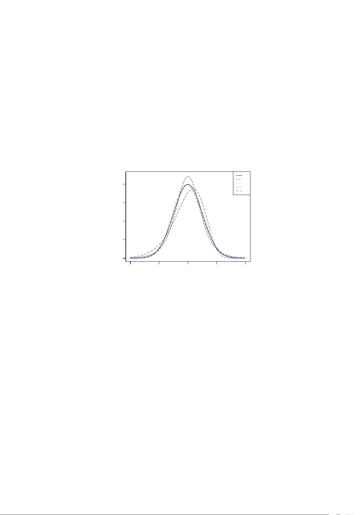
Go o dness-of-fit testing based on a w eigh ted b o otstrap: A fast large-sample alternativ e to the parametric b o otstrap Iv an Ko jadinovic Lab oratoire de math´ ematiques et applications, UMR CNRS 5142 Univ ersit ´ e de Pau et des P a ys de l’Adour B.P . 1155, 64013 Pau Cedex, F rance ivan.kojadinovic@univ-pau.fr Jun Y an Departmen t of Statistics Univ ersit y of Connecticut, 215 Glen bro ok Rd. U-4120 Storrs, CT 06269, USA jun.yan@uconn.edu Abstract The pro cess comparing the empirical cumulativ e distribution function of the sample with a parametric estimate of the cum ulative distribution function is kno wn as the empiric al pr o c ess with estimate d p ar ameters and has been extensively em- plo y ed in the literature for go odness-of-fit testing. The simplest wa y to carry out suc h go odness-of-fit tests, esp ecially in a m ultiv ariate setting, is to use a p ar ametric b o otstr ap . Although very easy to implement, the parametric b o otstrap can b ecome v ery computationally exp ensiv e as the sample size, the n umber of parameters, or the dimension of the data increase. An alternativ e resampling tec hnique based on a fast weighte d b o otstr ap is proposed in this paper, and is studied b oth theoretically and empirically . The outcome of this w ork is a generic and computationally efficien t multiplier go o dness-of-fit pro cedure that can b e used as a large-sample alternative to the parametric b ootstrap. In order to approximately determine ho w large the sample size needs to be for the parametric and w eigh ted b o otstraps to ha ve roughly equiv alen t p o wers, extensive Mon te Carlo experiments are carried out in dimension one, t w o and three, and for mo dels containing up to nine parameters. The com- putational gains resulting from the use of the prop osed multiplier go o dness-of-fit pro cedure are illustrated on triv ariate financial data. A by-product of this work is a fast large-sample goo dness-of-fit pro cedure for the biv ariate and triv ariate t distribution whose degrees of freedom are fixed. Key wor ds and phr ases: asymptotically linear estimator, empirical pro cess, multi- plier central limit theorem, multiv ariate t distribution. 1 1 In tro duction Let M = { F θ : θ ∈ O } b e a parametric family of cum ulative distribution functions (c.d.f.s) on R d , where O is an op en subset of R p , for some integers d ≥ 1 and p ≥ 1. Giv en a sample X 1 , . . . , X n of i.i.d. random vectors on R d with common c.d.f. F , w e are in terested in testing H 0 : F ∈ M against H 1 : F 6∈ M using statistics based on the empirical pro cess F n ( x ) = √ n { F n ( x ) − F θ n ( x ) } , x ∈ R d , (1) where F n ( x ) = 1 n n X i =1 1 ( X i ≤ x ) , x ∈ R d , is the empirical c.d.f. computed from the random sample X 1 , . . . , X n , and F θ n is a para- metric estimator of F computed under the n ull h yp othesis that F b elongs to M , that is, under the assumption that there exists θ 0 ∈ O suc h that F = F θ 0 . The latter parametric estimator of F under H 0 is obtained from an estimator θ n of θ 0 based on X 1 , . . . , X n . The abov e problem has b een extensiv ely studied in the literature (see e.g. Darling, 1955; Kac, Kiefer, and W olfo witz, 1955; Sukhatme, 1972; Durbin, 1973; Stephens, 1976; Khmal- adze, 1981; Durbin, 1975) and is often referred to as the problem of go o dness of fit when p ar ameters ar e estimate d . Tw o test statistics that are frequen tly used are the Cram´ er–v on Mises statistic S n = n Z R d { F n ( x ) − F θ n ( x ) } 2 d F θ n ( x ) (2) and the Kolmogoro v-Smirno v statistic T n = √ n sup x ∈ R d | F n ( x ) − F θ n ( x ) | . (3) Minor v ariations of these will also b e considered in this work. One imp ortan t and enduring issue regarding tests of go o dness of fit based on (1) con- cerns the computation of critical v alues or p -v alues for statistics derived from F n . Indeed, under classical regularit y conditions that will b e explicitly stated in the forthcoming sec- tion, the weak limit of the pro cess giv en in (1) inv olv es a drift term that t ypically mak es go o dness-of-fit tests based on F n distribution-dep enden t. T o solv e this problem in the univ ariate case, Khmaladze (1981) prop osed to use the theory of martingales to transform F n to an asymptotically distribution-free pro cess. In the same con text, Durbin (1973, 1975) inv estigated sev eral approac hes to compute appro ximate critical v alues for the Kolmogorov-Smirno v statistic. The martingale trans- form of Khmaladze (1981) and Durbin (1975)’s approach based on appro ximate b oundary crossing probabilities are reviewed and compared in Park er (2010) when M is a lo cation- scale or a scale-shap e univ ariate family . F or tests based on the Cram´ er–v on Mises, the 2 Anderson–Darling or the W atson statistics, Stephens (1976) (see also Sukhatme, 1972; Stephens, 1974) used the fact that the asymptotic distributions of these statistics can b e expressed as a w eighted sum of χ 2 1 v ariables and explained in detail ho w to compute the unkno wn w eights when M is the univ ariate normal or the exp onen tial distribution. A generic, v ery simple to implemen t resampling tec hnique, that can b e used to carry out tests of go o dness of fit based on F n in a general m ultiv ariate setting, is the so-called p ar ametric b o otstr ap (see e.g. Romano, 1988; Stute, Gonz´ ales Manteiga, and Presedo Quindimil, 1993; Jogesh Babu and Rao, 2004; Genest and R´ emillard, 2008). T o fix ideas, let S n b e the test statistic and assume that it is a con tinuous functional of the empirical pro cess F n . W e shall thus write S n = φ ( F n ). F or some large integer N and giv en an estimator θ n of θ 0 based on X 1 , . . . , X n , the parametric b o otstrap consists of rep eating the follo wing steps for every k ∈ { 1 , . . . , N } : (a) Generate a random sample X ( k ) 1 , . . . , X ( k ) n from c.d.f. F θ n . (b) Let F ( k ) n and θ ( k ) n stand for the versions of F n and θ n estimated from the random sample X ( k ) 1 , . . . , X ( k ) n . (c) F orm an approximate realization of the test statistic under H 0 as S ( k ) n = φ ( F ( k ) n ), where F ( k ) n = √ n ( F ( k ) n − F θ ( k ) n ). With the con ven tion that large v alues of S n lead to the rejection of H 0 , an appro ximate p -v alue for the test is finally giv en b y N − 1 P N k =1 1 ( S ( k ) n ≥ S n ). When n , p or d are large, the ab ov e pro cedure can b ecome very computationally exp ensiv e as, for ev ery k ∈ { 1 , . . . , N } , it requires the generation of a random sample from F θ n and the estimation of θ from the generated data, b oth steps b eing p oten tially v ery time-consuming. A computationally more efficient approac h consists of using a weighte d b o otstr ap in the sense of Burk e (2000) and Horv´ ath, Kok oszk a, and Steinebach (2000) (see also Horv´ ath, 2000, and the references therein). This resampling technique, based on the multiplier cen tral limit theorem for empirical pro cesses (see e.g. v an der V aart and W ellner, 2000; Kosorok, 2008), w as recently used for assessing the goo dness of fit of copula mo dels in Ko jadinovic, Y an, and Holmes (2011). While b eing asymptotically equiv alent to the parametric b o otstrap under the n ull h yp othesis, it was found that, in the case of large samples, the use of the w eighted instead of the parametric bo otstrap could reduce the computing time from ab out a da y to min utes for certain m ultiv ariate m ultiparameter mo dels. The aim of this pap er is to in vestigate, b oth theoretically and empirically , go o dness- of-fit tests for multiv ariate distributions based on a weigh ted b o otstrap in the sense of Burk e (2000). F rom a practical p ersp ective, a large scale Mon te Carlo study was carried out in order to appro ximately determine the sample size from which the parametric and the weigh ted b o otstrap ha v e roughly the same p o wer. F or small samples, the parametric b o otstrap usually app ears more p ow erful, and, since it t ypically has an acceptable com- putational cost in that case, it is the recommended approach. F or larger samples, the use 3 of the parametric b o otstrap can b ecome v ery tedious in practice and the deriv ed faster multiplier go o dness-of-fit pro cedure app ears as a natural alternative. The pap er is organized as follo ws. In the second section, to extend the breadth of the approac h, the theoretical results establishing the v alidity of the approac h are stated in the con text of the theory of empirical pro cesses as presented for instance in v an der V aart and W ellner (2000). The results of a large-scale sim ulation study are partially rep orted in the third section for univ ariate, biv ariate and triv ariate data sets and parametric c.d.f. families with up to nine parameters. The last section is dev oted to a detailed illustration on real financial data. All the pro ofs and computational details are relegated to the app endices. Note finally that the co de of all the tests studied in this work will b e do cumented and released as an R pack age accompan ying the pap er. 2 The w eigh ted b o otstrap for go o dness-of-fit testing T o extend the breadth of our study , w e shall work in the framew ork of the theory of empirical pro cesses as presented for instance in v an der V aart and W ellner (2000) or Kosorok (2008). Giv en a random sample X 1 , . . . , X n from a probability distribution P on R d , the empirical measure is defined to b e P n = n − 1 P n i =1 δ X i , where δ x is the measure that assigns a mass of 1 at x and zero elsewhere. F or a measurable function f : R d → R , P n f denotes the exp ectation of f under P n , and P f the exp ectation under P , i.e., P n f = 1 n n X i =1 f ( X i ) and P f = Z f d P . The empirical pro cess ev aluated at f is then defined as G n f = √ n ( P n f − P f ). As w e con tin ue, F denotes a P -Donsker class of measurable functions, whic h means that the sequence of pro cesses { G n f : f ∈ F } con verges w eakly to a P -Brownian bridge { G P f : f ∈ F } in the space ` ∞ ( F ) of b ounded functions from F to R equipp ed with the uniform metric in the sense of Definition 1.3.3 of v an der V aart and W ellner (2000). F ollo wing usual notational con ven tions, this weak conv ergence will simply b e denoted b y G n G P in ` ∞ ( F ). By taking F to b e the class of indicator functions of low er-left orthan ts in R d , i.e., F = { x 7→ 1 ( x ≤ t ) : t ∈ R d } with R = R ∪ {−∞ , ∞} , one recov ers a more classical version of Donsk er’s theorem stating that √ n ( F n − F ), where F is the c.d.f. asso ciated with P , conv erges weakly in the space ` ∞ ( R d ) of b ounded functions on R d to an F -Bro wnian bridge β , i.e., a tight cen tered Gaussian pro cess with co v ariance function E { β ( x ) β ( y ) } = F ( x ∧ y ) − F ( x ) F ( y ), x, y ∈ R d . The adv antage of working in this general framework is that the forthcoming results remain v alid for an y P -Donsk er class F . Although the collection of all indicator functions of low er-left orthants in R d ma y app ear as a natural choice for F in the go o dness-of-fit framew ork under consideration, other choices might b e of interest such as the class of indicator functions of closed balls, rectangles or half-spaces (see Romano, 1988, for a related discussion regarding the choice of F ). 4 In the rest of the paper, conv ergence in probabilit y is to be understo o d in outer probabilit y (see e.g. v an der V aart, 1998, Chapter 18). 2.1 Theoretical results Giv en i.i.d. random v ariables Z 1 , . . . , Z n with mean 0, v ariance 1, satisfying R ∞ 0 { P ( | Z 1 | > x ) } 1 / 2 d x < ∞ , and indep endent of the random sample X 1 , . . . , X n , the follo wing multi- plier v ersions of G n will b e of interest: G 0 n = 1 √ n n X i =1 Z i ( δ X i − P ) and G 00 n = 1 √ n n X i =1 ( Z i − ¯ Z ) δ X i , (4) where ¯ Z = n − 1 P n i =1 Z i . Let { P θ : θ ∈ O} b e an iden tifiable family of distributions, where O is an op en subset of R p , and let { ψ θ : θ ∈ O } b e a class of measurable functions from R d to R p . Assume additionally that (A1) for an y θ 0 ∈ O , the map θ 7→ P θ from R p to ` ∞ ( F ) is F r ´ ec het differentiable at θ 0 , i.e, there exists a map ˙ P θ 0 : F → R p suc h that sup f ∈F | P θ f − P θ 0 f − ( θ − θ 0 ) > ˙ P θ 0 f | = o ( k θ − θ 0 k ) as θ → θ 0 , (A2) for an y θ 0 ∈ O , sup f ∈F k ˙ P θ f − ˙ P θ 0 f k = o (1) as θ → θ 0 , (A3) for an y θ 0 ∈ O , there exists a δ > 0 suc h that the class of measurable functions { ψ θ : k θ − θ 0 k < δ } is P -Donsk er, (A4) for an y θ 0 ∈ O , Z k ψ θ ( x ) − ψ θ 0 ( x ) k 2 d P ( x ) = o (1) as θ → θ 0 , (A5) for an y θ 0 ∈ O and a random sample X 1 , . . . , X n from P θ 0 , θ n is an estimator of θ 0 that is asymptotically linear with influence function ψ θ 0 , i.e., √ n ( θ n − θ 0 ) = 1 √ n n X i =1 ψ θ 0 ( X i ) + o P θ 0 (1) , with P θ 0 ψ θ 0 = 0 and P θ 0 k ψ θ 0 k 2 < ∞ . The following t wo propositions, pro ved in App endix A, are at the ro ot of the go o dness- of-fit pro cedure to b e given in the next subsection. 5 Prop osition 1. L et X 1 , . . . , X n b e a r andom sample fr om the distribution P θ 0 for some θ 0 ∈ O . If Assumptions (A1)-(A5) ar e satisfie d, then  f 7→ √ n ( P n f − P θ n f ) , f 7→ G 0 n f − G 0 n ψ > θ n ˙ P θ n f , f 7→ G 00 n f − G 00 n ψ > θ n ˙ P θ n f  c onver ges we akly to  f 7→ G θ 0 f − G θ 0 ψ > θ 0 ˙ P θ 0 f , f 7→ G 0 θ 0 f − G 0 θ 0 ψ > θ 0 ˙ P θ 0 f , f 7→ G 0 θ 0 f − G 0 θ 0 ψ > θ 0 ˙ P θ 0 f  in { ` ∞ ( F ) } 3 , wher e G θ 0 , a P θ 0 -Br ownian bridge, is the we ak limit of G n , and G 0 θ 0 is an indep endent c opy of G θ 0 . Prop osition 2. L et X 1 , . . . , X n b e a r andom sample fr om a distribution P 6∈ { P θ : θ ∈ O } . If Assumptions (A1)-(A4) ar e satisfie d, and if ther e exists θ 0 ∈ O such that √ n ( θ n − θ 0 ) c onver ges in distribution under P , then sup f ∈F | √ n ( P n f − P θ n f ) | P → ∞ while  f 7→ G 0 n f − G 0 n ψ > θ n ˙ P θ n f , f 7→ G 00 n f − G 00 n ψ > θ n ˙ P θ n f  c onver ges we akly to  f 7→ G 0 P f − G 0 P ψ > θ 0 ˙ P θ 0 f , f 7→ G 0 P f − G 0 P ψ > θ 0 ˙ P θ 0 f  in { ` ∞ ( F ) } 2 , wher e G 0 P , a P -Br ownian bridge, is the we ak limit of G 0 n . 2.2 The go o dness-of-fit pro cedure Let us reformulate the results stated in Prop ositions 1 and 2 when F is the class of indicator functions of low er-left orthan ts in R d . As the empirical pro cess G 0 n defined in (4) dep ends on the unknown true distribution P , we shall only deal with the parts of the ab o v e results concerned with G 00 n . Thus, let F 00 n ( x ) = 1 √ n n X i =1 ( Z i − ¯ Z ) { 1 ( X i ≤ x ) − ψ > θ n ( X i ) ˙ F θ n ( x ) } , x ∈ R d , (5) where { F θ : θ ∈ O } = M is the set of c.d.f.s asso ciated with the parametric family of distributions { P θ : θ ∈ O } , and where, for an y x ∈ R d , ˙ F θ ( x ) is the gradien t of F θ ( x ) with resp ect to θ . Prop osition 1 then states that, if P = P θ 0 for some θ 0 ∈ O , then, under explicit regularity conditions, F n and F 00 n join tly con verge weakly in { ` ∞ ( R d ) } 2 to indep enden t copies of the same limit. Roughly sp eaking, under the n ull hypothesis H 0 : F ∈ M , where F is the c.d.f. asso ciated to P , the empirical pro cess F 00 n is close to b eing an indep endent cop y of F n . Ev ery new set of multipliers Z 1 . . . , Z n giv es a new appro ximate indep enden t cop y of F n . 6 Prop osition 2 is concerned with the b eha vior of F n and F 00 n under the alternativ e h yp othesis H 1 : F 6∈ M . If F 6∈ { F θ : θ ∈ O } , then, under explicit regularity condi- tions, any sensible statistic derived from F n will tend to infinity in probability b ecause sup x ∈ R d | F n ( x ) | P → ∞ , while F 00 n still con v erges w eakly . The verification of Assumptions (A1)-(A5) for a given family M of c.d.f.s is discussed in Section 2.3. No w, for illustration purp oses, let us assume that the test statistic is the Cram ´ er–von Mises statistic S n defined in (2). The results of Propositions 1 and 2 reform ulated abov e then suggest adopting the following goo dness-of-fit pro cedure: 1. Estimate θ 0 using an asymptotically linear estimator θ n . 2. Compute the test statistic S n = R R d { F n ( x ) } 2 d F θ n ( x ). 3. Then, for some large integer N , rep eat the following steps for ev ery k ∈ { 1 , . . . , N } : (a) Generate n i.i.d. random v ariates Z 1 , . . . , Z n with exp ectation 0, v ariance 1 and satisfying R ∞ 0 { P ( | Z 1 | > x ) } 1 / 2 d x < ∞ . (b) F orm an appro ximate realization of the test statistic under H 0 b y S ( k ) n = Z R d { F 00 n ( x ) } 2 d F θ n ( x ) , where F 00 n is defined in (5) 4. An appro ximate p -v alue for the test is then given b y N − 1 P N k =1 1 ( S ( k ) n ≥ S n ). The results giv en in the previous subsection imply that, under H 0 : F ∈ M and regularit y conditions, the ab o v e testing pro cedure will hold its level asymptotically . In- deed, ( S n , S (1) n , . . . , S ( N ) n ) conv erge join tly in distribution to indep endent copies of the same limit and, th us, the approximate p -v alue computed in Step 4 of the pro cedure will b e approximately standard uniform. On the other hand, under H 1 : F 6∈ M and regular- it y conditions, S n tends in probabilit y to infinity while ( S (1) n , . . . , S ( N ) n ) still con v erges in distribution. It follows that the appro ximate p -v alue will tend to zero in probability . The p oten tial computational adv an tage of the multiplier go o dness-of-fit pro cedure o ver the parametric bo otstrap is b est seen when Step 3 ab o v e is compared with the pro cedure recalled in the introduction. Roughly sp eaking, random n um b er generation from the fitted distribution and estimation of the parameters from the generated data at eac h parametric b o otstrap iteration is replaced b y the random generation of n m ultipliers, t ypically from the standard normal distribution or the uniform distribution on {− 1 , 1 } . T o obtain even faster go o dness-of-fits tests, we consider v ariations of S n and of the Kolmogoro v-Smirnov statistic T n defined in (3) given b y S ∗ n = Z R d { F n ( x ) } 2 d F n ( x ) = 1 n n X i =1 { F n ( X i ) } 2 = n X i =1 { F n ( X i ) − F θ n ( X i ) } 2 , (6) 7 and T ∗ n = max i ∈{ 1 ,...,n } | F n ( X i ) | = √ n max i ∈{ 1 ,...,n } | F n ( X i ) − F θ n ( X i ) | , (7) resp ectiv ely . When the go o dness-of-fit pro cedure is based on S ∗ n (resp. T ∗ n ), the multiplier realizations of Step 3 (b) are thus simply giv en by S ∗ , ( k ) n = Z R d { F 00 n ( x ) } 2 d F n ( x ) = 1 n n X i =1 { F 00 n ( X i ) } 2  resp. T ∗ , ( k ) n = max i ∈{ 1 ,...,n } | F 00 n ( X i ) |  . 2.3 Ab out the assumptions When F is the class of indicator functions of low er-left orthants in R d , Assumptions (A1) and (A2) concern the existence and the smo othness of the gradien t ˙ F θ . As discussed for instance in Genz and Haeusler (2006), these t wo conditions are typically satisfied if, for an y θ ∈ O , F θ has a p.d.f. f θ , and the function ( x, θ ) 7→ f θ ( x ) is smo oth in b oth x and θ . According to Example 19.7 in v an der V aart (1998), Assumption (A3) is satisfied if there exists a measurable function m such that k ψ θ 1 ( x ) − ψ θ 2 ( x ) k ≤ m ( x ) k θ 1 − θ 2 k , ∀ θ 1 , θ 2 ∈ { θ : k θ − θ 0 k < δ } , (8) with P | m | r < ∞ for some r > 0. The ab ov e inequality is satisfied for many M-estimators with P m 2 < ∞ . Assume furthermore that the functions θ 7→ ψ θ ( x ) are contin uously differen tiable and denote b y ˙ ψ θ ( x ) the gradien t of ψ θ ( x ) with resp ect to θ . Since θ 7→ ˙ ψ θ ( x ) is contin uous, then, as explained in v an der V aart (1998, page 53), the natural candidate for m is ˙ ψ ( x ) = sup θ : k θ − θ 0 k <δ k ˙ ψ θ ( x ) k . It then remains to v erify that P ˙ ψ 2 < ∞ . In other w ords, Assumption (A3) is typically satisfied if there exists a square-integrable function ˙ ψ such that k ˙ ψ θ ( x ) k ≤ ˙ ψ ( x ) when θ is close to θ 0 . F urthermore, if (8) holds, then, for k θ − θ 0 k < δ , Z k ψ θ ( x ) − ψ θ 0 ( x ) k 2 d P ( x ) ≤ k θ − θ 0 k Z m 2 ( x )d P ( x ) , and therefore, Assumption (A4) holds if P m 2 < ∞ . Assumption (A5) is related to the estimation of θ 0 under the null hypothesis, and is t ypically established in the theorems pro ving the asymptotic normalit y of M -estimators. It follows that (A5) holds under the assumptions of these theorems (see e.g. v an der V aart, 1998, Section 5.3). 3 Finite-sample p erformance In order to study the finite-sample performance of the prop osed m ultiplier go o dness-of-fit pro cedure, extensiv e Monte Carlo experiments w ere carried out in dimension one, tw o and three, for t w o- to nine-parameter families of absolutely con tin uous c.d.f.s. In all cases, the m ultipliers in the go o dness-of-fit procedure giv en in Section 2.2 are tak en from the standard normal distribution. 8 F or a given h yp othesized family M = { F θ : θ ∈ O } , the estimation of the unkno wn parameter vector θ 0 w as performed using numerical maximum likelihoo d estimation based on the Nelder-Mead optimization algorithm as implemen ted in the R optim routine (R Dev elopment Core T eam, 2011). Metho d-of-moment estimates of θ 0 w ere used as starting v alues. The use of maximum lik eliho o d estimation implies, under classical regularit y condi- tions (see e.g. v an der V aart, 1998, Section 5.5), that, for an y θ 0 ∈ O , the influence function ψ θ 0 app earing in Assumption (A5) is given b y ψ θ 0 ( x ) = I − 1 θ 0 ˙ f θ 0 ( x ) f θ 0 ( x ) 1 { f θ 0 ( x ) > 0 } , where f θ 0 is the probability densit y function (p.d.f.) asso ciated with F θ 0 , ˙ f θ 0 ( x ) is the gra- dien t of f θ 0 ( x ) with respect to θ 0 , and I θ 0 is the Fisher information matrix. Equiv alen tly , ψ θ 0 ( x ) can b e taken as I − 1 θ 0 times the gradien t of log f θ 0 ( x ) with resp ect to θ 0 . F rom Section 2.2, and in particular (5), w e see that ψ θ n is to b e computed instead of the unknown function ψ θ 0 . T o obtain a more generic implementation, all gradien ts, including ˙ F θ n , w ere computed numerically using Ric hardson’s extrap olation metho d as implemen ted in the R pac k age numDeriv (Gilb ert, 2011). As shall b e explained in more detail in the forthcoming subsections, this numerical approac h w as compared with a more precise implemen tation when M is the set of c.d.f.s of the m ultiv ariate t distribution with fixed degrees of freedom (d.f.). In b oth cases, the matrix I θ n w as estimated as the sample co v ariance matrix of the sample ˙ f θ n ( X 1 ) /f θ n ( X 1 ) , . . . , ˙ f θ n ( X n ) /f θ n ( X n ). 3.1 Univ ariate exp erimen ts In dimension one, four candidate test statistics were considered: n umerical appro xima- tions of S n and T n defined in (2) and (3), respectively , and the statistics S ∗ n and T ∗ n defined in (6) and (7), resp ectively . The numerical appro ximations of S n and T n are based on a uniform grid u 1 , . . . , u m on (0 , 1) which is transformed as y i = F − 1 θ n ( u i ), i ∈ { 1 , . . . , m } . The go o dness-of-fit pro cedure giv en in Section 2.2 is then based on the comparison of S n ≈ 1 m m X i =1 { F n ( y i ) } 2  resp. T n ≈ max i ∈{ 1 ,...,m } | F n ( y i ) |  , with the set of N multiplier realizations S ( k ) n ≈ 1 m m X i =1 { F 00 n ( y i ) } 2  resp. T ( k ) n ≈ max i ∈{ 1 ,...,m } | F 00 n ( y i ) |  , k ∈ { 1 , . . . , N } , where F 00 n is defined in (5). The grid size m w as set to 1000 in our exp eriments. In terms of distributions, five t wo-parameter families of absolutely con tinuous c.d.f.s w ere considered, namely the normal, t , logistic, gamma and W eibull distributions. The d.f. of the t distribution w ere fixed (to fiv e) to a v oid n umerical issues that arise when 9 attempting to estimate them (see e.g. Nadara jah and Kotz, 2008, for a review). These distributions are abbreviated b y N, T5, L, G and W as w e contin ue. F or data generation, the exp ectation and the v ariance of N were set to 10 and 1, resp ectiv ely . F or eac h of the remaining four distributions, its parameters w ere determined as approximate minimizers of the Kullbac k-Leibler divergence b etw een the p.d.f. of the distribution and the p.d.f. of the normal N (10 , 1). The exp ectation of T5 w as thus fixed to 10 and its dispersion (scale) parameter to 0.856. The location and scale parameters of L w ere fixed to 10 and 0.572, respectively . The shap e and rate parameters of G w ere set to 98.671 and 9.866, resp ectively , while, for W, the shap e and scale parameters were fixed to 10.618 and 10.452, resp ectiv ely . The parametrization of L, G and W used in this w ork corresp onds to the implementation of these distributions in the R statistical system. A plot of the p.d.f.s of the five data generating distributions is giv en in Figure 1. [Figure 1 ab out here.] F or each data generating distribution, 1000 random samples of size n w ere generated for n = 100, 200, 300, 400 and 500. Under eac h scenario, the five families men tioned ab o v e were hypothesized. F or eac h of the four test statistics, the prop osed multiplier go o dness-of-fit pro cedure (abbreviated b y MP as w e contin ue) w as compared with the parametric bo otstrap-based go o dness-of-fit pro cedure (abbreviated by PB). All the tests w ere carried out at the 5% level of significance. As the Cram´ er–v on Mises statistics S n and S ∗ n consisten tly outerp erformed the Kolmogoro v-Smirnov statistics T n and T ∗ n , we only report the rejection rates of the former in T able 1. The fiv e horizon tal blo cks of the table corresp ond to the five data generating distributions whose parameters w ere given previously . The first tw o columns contain the empirical p ow ers of the Shapiro-Wilk and Jarque-Bera tests of univ ariate normality . The empirical lev els of all the tests are in italic in the table. As can b e noticed, these are, o v erall, reasonably close to the 5% significance lev el ev en for small n . [T able 1 ab out here.] In terms of rejection rates, the tests based on S n and S ∗ n are, ov erall, very close. F rom a practical p ersp ectiv e, recall that the latter are easier to implemen t. Notice also that the tests based on PB are, o verall, more p ow erful than those based on MP for small n . Ho wev er, as n increases, the difference in rejection rate v anishes in most scenarios. These results suggest that the multiplier pro cedure can b e safely used as a large-sample alternativ e to the parametric b o otstrap in dimension one. T o complemen t the previous study , the lev els of the tests were also inv estigated for hea vy-tailed and strongly asymmetric distributions. More sp ecifically , the levels of the tests were estimated from 1000 random samples of size n generated from the standard t distribution with fixed d.f. ν ∈ { 1 , 2 , 3 , 4 , 5 } , and from the gamma distribution with rate parameter 0.5 and shap e parameter in { 1 , 2 , 4 , 8 , 16 } . The obtained rejection rates (not rep orted) w ere found to b e reasonably close to the 5% nominal lev el in all scenarios and for all n ∈ { 100 , 200 , 300 , 400 , 500 } . 10 3.2 Biv ariate and triv ariate exp erimen ts In the biv ariate and triv ariate simulations, only the go o dness-of-fit pro cedures based on S ∗ n and T ∗ n w ere used, and five families of distributions w ere considered. In addition to the multiv ariate normal (abbreviated by N) and the m ultiv ariate t distribution with fiv e d.f. (abbreviated by T5), three absolutely contin uous families were constructed from Sklar (1959)’s represen tation theorem. The latter result states that any m ultiv ariate c.d.f. F : R d → [0 , 1] whose marginal c.d.f.s F 1 , . . . , F d are con tin uous can b e expressed in terms of a unique d -dimensional copula C as F ( x ) = C { F 1 ( x 1 ) , . . . , F d ( x d ) } , x = ( x 1 , . . . , x d ) ∈ R d . A first non-Gaussian family was obtained by taking F 1 , . . . , F d to b e gamma and C to be a normal copula, a second c hoice w as to tak e F 1 , . . . , F d to b e t with fiv e d.f. and C to b e a normal copula, while a third family w as obtained by taking F 1 , . . . , F d normal and C to b e a Clayton copula. These three families are resp ectiv ely abbreviated by GN, T5N and NC as we contin ue. Notice that the multiv ariate normal N is obtained b y taking F 1 , . . . , F d normal and C normal, while T5, the multiv ariate t with fiv e d.f., is obtained b y taking F 1 , . . . , F d to b e t with five d.f. and C to b e a t copula with five d.f. In dimension t wo, all fiv e families ha v e five parameters: t w o parameters p er margin and one parameter for the copula. In dimension three, N, T5, GN and T5N ha ve nine parameters (tw o parameters p er margin and three correlation coefficients for the copulas), while NC has seven parameters (t w o parameters p er margin and one parameter for the Cla yton copula). F or data generation, the margins of the distributions N and NC were taken to b e the N (10 , 1), the gamma margins of GN w ere c hosen to hav e shap e and rate parameters equal to 98.671 and 9.866, resp ectively , while the margins of T5 and T5N were set to ha ve exp ectation 10 and disp ersion 0.856. In order to study the effect of the dependence on the tests, the correlation co efficients of the normal and t copulas were first tak en equal to 0.309 and then to 0.588, while the parameter of the Cla yton copula used to construct NC was first taken equal to 0.5 and then to 1.333. This corresp onds to requiring that the v alue of Kendall’s tau (denoted b y τ in the tables) for all biv ariate margins of the copulas is first equal to 0.2 and then to 0.4. F or N and T5, random num b er generation and the computation of the p.d.f. and the c.d.f. was p erformed using the excellen t mvtnorm R pac k age (Genz, Bretz, Miw a, Mi, Leisch, Scheipl, and Hothorn, 2011). F or NC, GN and T5N, the copula pack age (Ko jadinovic and Y an, 2010) w as used in addition. The results for dimension t wo are giv en in T able 2. The columns SW contain the rejec- tion rates of the m ultiv ariate extension of the Shapiro–Wilk test prop osed b y Villasenor- Alv a and Gonzalez-Estrada (2009) and implemen ted in the R pack age mvShapiroTest (Gonzalez-Estrada and Villasenor-Alv a, 2009). Unlike in dimension one, the comparison b et w een the m ultiplier pro cedure and the parametric b o otstrap was carried out only in the situation where a biv ariate normal distribution is hypothesized. In that case, the maxim um likelihoo d estimates are the sample mean and the sample co v ariance matrix, and these were used in the parametric bo otstrap to decrease its computational cost. The rejection rates of the m ultiplier pro cedure and the parametric b o otstrap are rep orted in 11 the columns N-MP and N-PB, resp ectively . The parametric b o otstrap app ears clearly more p o werful than the multiplier but, as in dimension one, the difference in rejection rate tends to v anish as n reac hes 500. Also, the comparison of the columns SW, N-MP and N-PB rev eals, without surprise, that the sp ecialized m ultiv ariate Shapiro–Wilk test is generally more p ow erful than its tw o generic comp etitors. [T able 2 ab out here.] By lo oking at the entries in italic in T able 2, we see that the m ultiplier pro cedure is, o verall, to o conserv ativ e for smaller n , but that the agreemen t b etw een the empirical lev els and the 5% significance lev el improv es as n increases. The effect of stronger dep endence on the p ow er is v ariable. F or instance, when data are generated from NC, the families N, T5N, T5 and GMN are easier to reject for τ = 0 . 4 than for τ = 0 . 2, but, when the true distribution is N, it is easier to reject T5N and T5 in the case of w eaker dep endence. Notice finally that, as could hav e b een exp ected, it is very difficult to distinguish betw een T5 from T5N for these sample sizes. The results of the triv ariate Monte Carlo simulations are given in T able 3. This time, to mak e the computational cost of the sim ulation acceptable, only the multiplier pro cedure was used. By lo oking at the en tries in italic, we can see, as in the biv ariate case, that the tests are, ov erall, to o conserv ativ e, but that the empirical lev els impro ve as n increases. A comparison with T able 2 also reveals that the rejection rates are higher in dimension three than in dimension t w o, which suggests that the differences betw een the distributions are easier to detect as d increases from 2 to 3. F rom a more practical p ersp ective, we see that the empirical p ow ers approach 100% as n reaches 500 in man y scenarios under the alternativ e hypothesis. [T able 3 ab out here.] 3.3 The case of the m ultiv ariate t distribution When M is the set of c.d.f.s from the m ultiv ariate t distribution with fixed d.f., tw o differen t wa ys of computing the gradients ˙ F θ and ˙ f θ /f θ , θ ∈ O , were considered. The first one is the generic approach mentioned earlier relying on Ric hardson’s extrap olation metho d as implemented in the R pack age numDeriv . This n umerical metho d requires n umerous ev aluations of the c.d.f. and the log p.d.f. of the multiv ariate t as it is based on finite differences. F or that reason, in the triv ariate experiments, the algorithm pa- rameter of the pmvt and pmvnorm functions of the mvtnorm pac k age w as set to TVPACK (Genz, 2004) instead of the default algorithm GenzBretz . Indeed, the latter is based on randomized quasi Monte Carlo metho ds (Genz and Bretz, 1999, 2002) which implies that its results dep end on random num b er generation and are therefore not fully repro ducible. The second approac h, which is exp ected to b e more precise, is based, as explained in App endix B, on the fact that the gradien t ˙ f θ /f θ can b e computed analytically , and on the fact that the gradien t ˙ F θ can b e expressed in terms of the c.d.f. and the p.d.f. of the m ultiv ariate t . 12 These t wo approac hes w ere thoroughly compared and their results w ere found to b e v ery close. As could ha v e b een exp ected, the second more analytical approach is m uch faster as it requires significantly fewer ev aluations of the c.d.f. and the p.d.f. of the m ultiv ariate t . This asp ect will b e illustrated in the next section. Let us finally discuss the estimation of the parameters of the multiv ariate t with fixed d.f. ν using the Nelder-Mead algorithm. In dimension three for small ν ≥ 3, we noticed that the estimation of the nine parameters w as extremely sensitive to the choice of the starting v alues, and that the m ultiplier test tended to b e to o lib eral. Suc h issues w ere not observ ed for the other families of c.d.f.s used in the triv ariate sim ulations. Impro v ed results were obtained by changing the scale of the optimization using the parscale ar- gumen t of the R optim routine. The latter argumen t was set to the vector of starting v alues with a guard against v alues to o close to zero. Additional sim ulations w ere carried out for ν = 3, 5, 7, 10, 20 and 30 to study the empirical lev els of the multiplier test. T able 4 gives such empirical lev els when data are generated from biv ariate and triv ariate t distributions with ν d.f. fitted from the financial data studied in Section 4. As one can notice, in dimension t wo, the empirical levels are reasonably close to the 5% significance lev el. In dimension three how ever, the test is clearly to o lib eral for ν = 3 and migh t b e sligh tly too lib eral for ν = 5. W e could not determine whether a similar issue also affects the parametric bo otstrap for computational reasons. W e do ho wev er b elieve that the use of estimation pro cedures sp ecifically tailored to the m ultiv ariate t (see e.g. Nadara jah and Kotz, 2008, Section 3) would solv e this problem. [T able 4 ab out here.] 4 Illustration The results of the univ ariate, biv ariate and triv ariate exp erimen ts whose results w ere partially rep orted in the previous section hence suggest that the multiplier procedure can b e safely used as a large-sample alternative to the parametric b o otstrap. T o illustrate the computational adv an tage of the multiplier pro cedure ov er the para- metric bo otstrap, we consider the financial data analyzed in McNeil, F rey , and Em brech ts (2005, Chapter 5). These consist of fiv e y ears of daily log-returns (1996-2000) for the Intel (INTC), Microsoft (MSFT) and General Electric (GE) stocks, whic h giv es a triv ariate sample of size n = 1262. Univ ariate goo dness-of-fit tests for N, T5, T10, T20 and L were first applied to the In tel log-return data. The other distributions used in the univ ariate sim ulations w ere not considered as their supp ort is (0 , ∞ ). Appro ximate p -v alues and execution times are rep orted in the first horizontal blo ck of T able 5. The execution times are obtained from our R implemen tations of the m ultiplier procedure and of the para- metric b o otstrap. As one can see, the approximate p -v alues of the m ultiplier pro cedure and the parametric bo otstrap are fairly close, and the execution times are of the same order of magnitude. The latter observ ation is essentially due to the fact that (i) the n umerical estimation of the parameters of the hypothesized distributions (on which the parametric b o otstrap hea vily relies) is reasonably fast in dimension one, and (ii) the gra- dien ts needed in the multiplier procedure are computed numerically using the numDeriv 13 pac k age as explained previously . Biv ariate goo dness-of-fit tests for N, NC, T10N, T5, T10 and T20 were then applied to the biv ariate log-returns of the In tel and General Electric sto c ks. Again, the approximate p -v alues of the m ultiplier pro cedure and the parametric b o otstrap are fairly close. This time, ho w ever, the computational adv antage of the mul- tiplier pro cedure is obvious, in particular when T10N is hypothesized (1.6 minutes v ersus 4.2 hours for the parametric b o otstrap on one 2.33 GHz pro cessor). The approximate p -v alues and executions times in italic in T able 5 w ere obtained using the m ultiplier pro- cedure based on the gradients computed using the more analytical approach describ ed in App endix B. Finally , go o dness-of-fit tests for N, NC, T10N, T5, T10 and T20 w ere applied to the triv ariate log-returns. F rom the third horizon tal blo c k of T able 5, we see that the computational adv antage of the multiplier is even more pronounced than in dimension t wo. F or T10N for instance, the execution of the m ultiplier pro cedure to ok 4.3 minutes while 16.6 hours were necessary to obtain an appro ximate p -v alue using the parametric b o otstrap. [T able 5 ab out here.] The en tries in italic in T able 5 sho w that the execution times of the generic implemen- tation of the m ultiplier pro cedure based on the numDeriv pack age can b e significan tly lo wered at the exp ense of more analytical and programming w ork. F ormulas similar to or simpler than those given in App endix B could b e obtained for all the multiv ariate distributions considered in this work. The appro ximate p -v alues giv en in the third horizontal blo ck of T able 5 indicate that there is very little evidence against the triv ariate distributions T5 and T10. On the basis of these tests, w e can conclude that a triv ariate t distribution whose d.f. are close to 10 is a plausible mo del for these financial data. Ac kno wledgmen ts The authors would lik e to thank the asso ciate editor and a referee for their insightful and constructiv e commen ts as well as Lauren t Bordes for fruitful discussions. A Pro ofs of the prop ositions The follo wing lemma will b e used in the pro ofs of Prop ositions 1 and 2. Lemma 1. L et X 1 , . . . , X n b e a r andom sample fr om a distribution P that may or may not b elong to { P θ : θ ∈ O } . If Assumptions (A1)-(A4) ar e satisfie d, and if ther e exists θ 0 ∈ O such that θ n c onver ges in pr ob ability to θ 0 under P , then  f 7→ G n f − G n ψ > θ 0 ˙ P θ 0 f , f 7→ G 0 n f − G 0 n ψ > θ n ˙ P θ n f , f 7→ G 00 n f − G 00 n ψ > θ n ˙ P θ n f  c onver ges we akly to  f 7→ G P f − G P ψ > θ 0 ˙ P θ 0 f , f 7→ G 0 P f − G 0 P ψ > θ 0 ˙ P θ 0 f , f 7→ G 0 P f − G 0 P ψ > θ 0 ˙ P θ 0 f  14 in { ` ∞ ( F ) } 3 , wher e G P , a P -Br ownian bridge, is the we ak limit of G n , and G 0 P is an indep endent c opy of G P . Pr o of. F rom Assumption (A3), { ψ θ 0 } is P -Donsker. It follows that the class G obtained as the union of F and the p comp onents of ψ θ 0 is P -Donsk er. F rom the functional multiplier cen tral limit theorem (see e.g. Kosorok, 2008, Theorem 10.1 and Corollary 10.3), we then ha ve that ( G n , G 0 n , G 00 n ) ( G P , G 0 P , G 0 P ) in { ` ∞ ( G ) } 3 . By the contin uous mapping theorem, it first follows that ( G n , G n ψ θ 0 , G n , G 0 n ψ θ 0 , G n , G 00 n ψ θ 0 )  G θ 0 , G θ 0 ψ θ 0 , G 0 θ 0 , G 0 θ 0 ψ θ 0 , G 0 θ 0 , G 0 θ 0 ψ θ 0  in { ` ∞ ( F ) × R p } 3 , and then that  f 7→ G n f − G n ψ > θ 0 ˙ P θ 0 f , f 7→ G 0 n f − G 0 n ψ > θ 0 ˙ P θ 0 f , f 7→ G 00 n f − G 00 n ψ > θ 0 ˙ P θ 0 f  (9) con verges w eakly to  f 7→ G P f − G P ψ > θ 0 ˙ P θ 0 f , f 7→ G 0 P f − G 0 P ψ > θ 0 ˙ P θ 0 f , f 7→ G 0 P f − G 0 P ψ > θ 0 ˙ P θ 0 f  (10) in { ` ∞ ( F ) } 3 . No w, from Assumption (A3), there exists a δ > 0 such that H = { ψ θ : k θ − θ 0 k < δ } is P -Donsk er. Let H k , k ∈ { 1 , . . . , p } , be the p comp onent classes of H . They are P -Donsk er by definition. Next, fix k ∈ { 1 , . . . , p } and let g b e a function from ` ∞ ( H k ) × H k → R defined by g ( z , ψ ) = z ( ψ ) − z ( ψ θ 0 ,k ), where ψ θ 0 ,k is the k th comp onen t of ψ θ 0 . As noted in v an der V aart (1998, pro of of Lemma 19.24), the set H k is a semimetric space with resp ect to metric L 2 ( P ) and the function g is con tin uous with resp ect to the pro duct semimetric on ` ∞ ( H k ) × H k at ev ery p oint ( z , ψ ) such that ψ 7→ z ( ψ ) is contin uous. F rom Assumption (A4), the fact that θ n con verges to θ 0 in probability , and Lemma 2.12 of v an der V aart (1998), we also hav e that ψ θ n ,k con verges in probabilit y to ψ θ 0 ,k in the space H k equipp ed with the metric L 2 ( P ). Since H k is P -Donsker, G 0 n G 0 P in ` ∞ ( H k ). Also, since θ n con verges to θ 0 in probability , the probability that ψ θ n ,k is in H k tends to 1. On that ev en t, it follo ws that ( G 0 n , ψ θ n ,k ) ( G 0 P , ψ θ 0 ,k ) in ` ∞ ( H k ) × H k . Since ψ k 7→ G 0 P ψ k is con tinuous at ev ery ψ k ∈ H k almost surely , the function g is con tinuous at almost every ( G 0 P , ψ θ 0 ,k ). By the contin uous mapping theorem, we obtain that g ( G 0 n , ψ θ n ,k ) = G 0 n ψ θ n ,k − G 0 n ψ θ 0 ,k g ( G 0 P , ψ θ 0 ,k ) = 0. Hence, w e hav e that G 0 n ψ θ n ,k − G 0 n ψ θ 0 ,k = o P (1) , k ∈ { 1 , . . . , p } . (11) Similarly , we ha ve that G 00 n ψ θ n ,k − G 00 n ψ θ 0 ,k = o P (1) , k ∈ { 1 , . . . , p } . (12) F rom Assumption (A2) and the fact θ n con verges to θ in probabilit y , we also ha ve that sup f ∈F k ˙ P θ n f − ˙ P θ 0 f k = o P (1) . (13) Finally , combining (9) and (10) with (11), (12) and (13), we obtain the desired result. 15 W e can now pro ve Proposition 1 and 2. Pro of of Prop osition 1. Assumption (A5) implies that θ n con verges to θ 0 in proba- bilit y . F rom Assumption (A1) and Lemma 2.12 of v an der V aart (1998), w e then ha ve that sup f ∈F | P θ n f − P θ 0 f − ( θ n − θ 0 ) > ˙ P θ 0 f | = k θ n − θ 0 k o P θ 0 (1) , whic h in turn is implies that sup f ∈F | √ n ( P θ n f − P θ 0 f ) − √ n ( θ n − θ 0 ) > ˙ P θ 0 f | = o P θ 0 (1) , since k √ n ( θ n − θ 0 ) k = O P θ 0 (1) from Assumption (A5) and the contin uous mapping the- orem. It follows that √ n ( P n − P θ n ) = √ n ( P n − P θ 0 ) − √ n ( P θ n − P θ 0 ) = √ n ( P n − P θ 0 ) − √ n ( θ n − θ 0 ) > ˙ P θ 0 + R n , where sup f ∈F | R n f | = o P θ 0 (1). Using Assumption (A5) again, we obtain that √ n ( P n f − P θ n f ) = G n f − G n ψ > θ 0 ˙ P θ 0 f + Q n f , f ∈ F , (14) where sup f ∈F | Q n f | = o P θ 0 (1). The result is finally an immediate consequence of Lemma 1. Pro of of Prop osition 2. W rite √ n ( P n − P θ n ) = √ n ( P n − P ) − √ n ( P θ n − P θ 0 ) − √ n ( P θ 0 − P ) . (15) The first term conv erges weakly to G P in ` ∞ ( F ). Now, the conv ergence in distribution of √ n ( θ n − θ 0 ) implies that θ n con verges in probability to θ 0 . Hence, proceeding as in the pro of of Prop osition 1, Assumption (A1) implies that sup f ∈F | √ n ( P θ n f − P θ 0 f ) − √ n ( θ n − θ 0 ) > ˙ P θ 0 f | = o P (1) , whic h in turn implies that the second term in (15) conv erges w eakly in ` ∞ ( F ). How ever, since P 6∈ { P θ : θ ∈ O} , the suprem um ov er F of the third term diverges, whic h implies that sup f ∈F | √ n ( P n f − P θ n f ) | P → ∞ . The second part of the prop osition is an immediate consequence of Lemma 1. B Computational details for the m ultiv ariate t The p.d.f. of the cen tered d -dimensional multiv ariate t with disp ersion matrix Σ and ν d.f. is giv en b y t ν, Σ ( x ) = Γ  ν + d 2  ( π ν ) d 2 Γ  ν 2  | Σ | 1 2  1 + 1 ν x > Σ − 1 x  − ν + d 2 , x ∈ R d . (16) 16 Let T ν, Σ denote the corresp onding c.d.f. It is easy to v erify that the c.d.f. of the m ultiv ari- ate t with ν d.f., expectation v ector ( µ 1 , . . . , µ d ), dispersions λ 1 , . . . , λ d and correlation matrix Σ is then given b y T ν, Σ ,µ,λ ( x ) = T ν, Σ  x 1 − µ 1 λ 1 , . . . , x d − µ d λ d  , x ∈ R d . The corresp onding p.d.f. is thus t ν, Σ ,µ,λ ( x ) = d Y j =1 λ j ! − 1 t ν, Σ  x 1 − µ 1 λ 1 , . . . , x d − µ d λ d  , x ∈ R d . Let us first explain how, for an y x ∈ R d , the gradien t of T ν, Σ ,µ,λ ( x ) with respect to all the parameters except ν can b e computed. Let j ∈ { 1 , . . . , d } , and, for an y x ∈ R d , let T ( j ) ν, Σ ( x ) = ∂ T ν, Σ ( x ) /∂ x j . Also, let Σ − j, − j b e a ( d − 1) × ( d − 1) matrix obtained from Σ b y removing its j th ro w and j th column, Σ − j,j b e a ( d − 1) × 1 matrix obtained from Σ b y remo ving its j th ro w and k eeping only its j th column, and Σ j, − j = Σ > − j,j . F rom Nadara jah and Kotz (2005, page 66), if X is standard m ultiv ariate t with ν d.f. and correlation matrix Σ, then, conditionally on X j = x j , w e ha v e that s ν + 1 ν + x 2 j ( X − j − x j Σ − j,j ) is m ultiv ariate cen tered t with ν + 1 degrees of freedom and disp ersion matrix Λ j = Σ − j, − j − Σ − j,j Σ j, − j . Hence, T ( j ) ν, Σ ( x ) = t ν ( x j ) T ν +1 , Λ j s ν + 1 ν + x 2 j ( x − j − x j Σ − j,j ) ! , x ∈ R d . Using the previous expression, it is therefore p ossible to compute ∂ T ν, Σ ,µ,λ ( x ) ∂ µ j = − λ − 1 j T ( j ) ν, Σ  x 1 − µ 1 λ 1 , . . . , x d − µ d λ d  , x ∈ R d , and ∂ T ν, Σ ,µ,λ ( x ) ∂ λ 2 j = − x j − µ j 2 λ 3 j T ( j ) ν, Σ  x 1 − µ 1 λ 1 , . . . , x d − µ d λ d  , x ∈ R d . Also, let ρ i,j b e an off-diagonal element of the correlation matrix Σ. Then, ∂ T ν, Σ ,µ,λ ( x ) ∂ ρ i,j = ∂ T ν, Σ  x 1 − µ 1 λ 1 , . . . , x d − µ d λ d  ∂ ρ i,j , x ∈ R d , and, for any x ∈ R d , ∂ T ν, Σ ( x ) /∂ ρ i,j can b e computed using the Plac kett formula for the m ultiv ariate t (see Genz, 2004; Ko jadinovic and Y an, 2011, Prop osition 1). 17 Let us now discuss the computation, for any x ∈ R d , of the gradien t of log t ν, Σ ,µ,λ ( x ) with resp ect to all the parameters except ν . Let j ∈ { 1 , . . . , d } , and, for an y x ∈ R d , let t ( j ) ν, Σ ( x ) = ∂ t ν, Σ ( x ) /∂ x j . Starting from (16), one obtains that t ( j ) ν, Σ ( x ) = − ( ν + d ) x > Σ − 1 e j ν + x > Σ − 1 x t ν, Σ ( x ) , x ∈ R d , where e j is the unit v ector of R d whose i th comp onen t is 1 if i = j and 0 otherwise. Using the previous expression, it is therefore p ossible to compute ∂ log t ν, Σ ,µ,λ ( x ) ∂ µ j = − λ − 1 j t ( j ) ν, Σ  x 1 − µ 1 λ 1 , . . . , x d − µ d λ d  t ν, Σ  x 1 − µ 1 λ 1 , . . . , x d − µ d λ d  , x ∈ R d , and ∂ log t ν, Σ ,µ,λ ( x ) ∂ λ 2 j = − 1 2 λ 2 j − x j − µ j 2 λ 3 j t ( j ) ν, Σ  x 1 − µ 1 λ 1 , . . . , x d − µ d λ d  t ν, Σ  x 1 − µ 1 λ 1 , . . . , x d − µ d λ d  , x ∈ R d . Finally , starting again from (16), one obtains that ∂ t ν, Σ ( x ) ∂ ρ i,j = − 1 2 t ν, Σ ( x ) ( 1 | Σ | ∂ | Σ | ∂ ρ i,j + ( ν + d ) x > ∂ Σ − 1 ∂ ρ i,j x ν + x > Σ − 1 x ) , x ∈ R d . F rom Seb er (2008, Chap. 17) for instance, we ha ve that ∂ | Σ | ∂ ρ i,j = 2 K ij and that ∂ Σ − 1 ∂ ρ i,j = − r i r > j − r j r > i , where K ij is the cofactor of ρ i,j , and where r i is the i -th column of Σ − 1 . References M.D. Burke. Multiv ariate tests-of-fit and uniform confidence bands using a weigh ted b o otstrap. Statistics and Pr ob ability L etters , 46:13–20, 2000. D.A. Darling. The Cram ´ er–Smirnov test in the parametric case. A nnals of Mathematic al Statistics , 26:1–20, 1955. J. Durbin. W eak conv ergence of the sample distribution function when parameters are estimated. Annals of Statistics , 1:279–290, 1973. J. Durbin. Kolmogorov–Smirno v tests when parameters are estimated with applications to tests of exp onentialit y and tests on spacings. Biometrika , 62(1):5–22, 1975. C. Genest and B. R´ emillard. V alidit y of the parametric b o otstrap for go o dness-of-fit testing in semiparametric mo dels. Annales de l’Institut Henri Poinc ar´ e: Pr ob abilit´ es et Statistiques , 44:1096–1127, 2008. 18 A. Genz. Numerical computation of rectangular biv ariate and triv ariate normal and t probabilities. Statistics and Computing , 14:251–260, 2004. A. Genz and F. Bretz. Numerical computation of m ultiv ariate t-probabilities with appli- cation to p o w er calculation of multiple contrasts. Journal of Statistic al Computation and Simulation , 63:361–378, 1999. A. Genz and F. Bretz. Metho ds for the computation of multiv ariate t-probabilities. Journal of Computational and Gr aphic al Statistics , 11:950–971, 2002. A. Genz, F. Bretz, T. Miwa, X. Mi, F. Leisc h, F. Sc heipl, and T. Hothorn. mvtnorm: Multivariate normal and t distribution , 2011. URL http://CRAN.R- project.org/ package=mvtnorm . R pack age v ersion 0.9-9991. M. Genz and E. Haeusler. Empirical pro cesses with estimated parameters under auxiliary information. Journal of Computational and Applie d Mathematics , 186:191–216, 2006. P aul Gilb ert. numDeriv: A c cur ate Numeric al Derivatives , 2011. URL http://CRAN. R- project.org/package=numDeriv . R pac k age version 2010.11-1. E. Gonzalez-Estrada and J.A. Villasenor-Alv a. mvShapir oT est: Gener alize d Shapir o-Wilk test for multivariate normality , 2009. URL http://CRAN.R- project.org/package= mvShapiroTest . R pack age v ersion 0.0.1. L. Horv´ ath. Appro ximations for hybrids of empirical and partial sums pro cesses. Journal of Statistic al Planning and Infer enc e , 88:1–18, 2000. L. Horv´ ath, P . Kok oszk a, and J. Steinebac h. Appro ximations for w eighted b o otstrap pro cesses with an application. Statistics and Pr ob ability L etters , 48:59–70, 2000. G. Jogesh Babu and C.R. Rao. Go o dness-of-fit tests when parameters are estimated. Sankhya: The Indian Journal of Statistics , 66:63–74, 2004. M. Kac, J. Kiefer, and J. W olfowitz. On tests of normality and other tests of go o dness of fit based on distance methods. A nnals of Mathematic al Statistics , 26:189–211, 1955. E. Khmaladze. Martingale approach in the theory of go o dness-of-fit tests. The ory of Pr ob ability and its Applic ations , 26(2):240–257, 1981. I. Ko jadino vic and J. Y an. Mo deling multiv ariate distributions with con tin uous margins using the copula R pack age. Journal of Statistic al Softwar e , 34(9):1–20, 2010. I. Ko jadinovic and J. Y an. A go o dness-of-fit test for m ultiv ariate m ultiparameter copulas based on multiplier central limit theorems. Statistics and Computing , 21(1):17–30, 2011. I. Ko jadinovic, J. Y an, and M. Holmes. F ast large-sample go o dness-of-fit for copulas. Statistic a Sinic a , 21(2):841–871, 2011. M.R. Kosorok. Intr o duction to empiric al pr o c esses and semip ar ametric infer enc e . Springer, New Y ork, 2008. 19 A.J. McNeil, R. F rey , and P . Em brech ts. Quantitative risk management . Princeton Univ ersity Press, New Jersey , 2005. S. Nadara jah and S. Kotz. Mathematical prop erties of the m ultiv ariate t distribution. A cta Applic andae Mathematic ae , 89:53–84, 2005. S. Nadara jah and S. Kotz. Estimation metho ds for the m ultiv ariate t distribution. A cta Applic andae Mathematic ae , 102:99–118, 2008. T. Park er. A comparison of alternative approac hes to sup-norm go o dness of fit tests with estimated parameters. Working p ap er , 2010. R Dev elopment Core T eam. R: A L anguage and Envir onment for Statistic al Computing . R F oundation for Statistical Computing, Vienna, Austria, 2011. URL http://www. R- project.org . ISBN 3-900051-07-0. J.P . Romano. A b o otstrap reviv al of some nonparametric distance tests. Journal of the A meric an Statistic al Asso ciation , 83(403):698–708, 1988. G.A.F. Seber. A matrix handb o ok for statisticians . Wiley Series in Probabilit y and Statistics. Wiley , 2008. A. Sklar. F onctions de r ´ epartition ` a n dimensions et leurs marges. Public ations de l’Institut de Statistique de l’Universit´ e de Paris , 8:229–231, 1959. M.A. Stephens. EDF statistics for go o dness-of-fit and some comparisons. Journal of the A meric an Statistic al Asso ciation , 69:730–737, 1974. M.A. Stephens. Asymptotic results for go o dness-of-fit statistics with unknown parame- ters. Annals of Statistics , 4:357–369, 1976. W. Stute, W. Gonz´ ales Man teiga, and M. Presedo Quindimil. Bo otstrap based go o dness- of-fit tests. Metrika , 40:243–256, 1993. S. Sukhatme. F redholm determinant of a p ositive definite k ernel of a sp ecial t yp e and its application. Annals of Mathematic al Statistics , 43:1914–1926, 1972. A.W. v an der V aart. Asymptotic statistics . Cam bridge Univ ersit y Press, 1998. A.W. v an der V aart and J.A. W ellner. We ak c onver genc e and empiric al pr o c esses . Springer, New Y ork, 2000. Second edition. J.A. Villasenor-Alv a and E. Gonzalez-Estrada. A generalization of Shapiro–Wilk’s test for multiv ariate normalit y . Communic ations in Statistics: The ory and Metho ds , 38: 1870–1883, 2009. 20 6 8 10 12 14 0.0 0.1 0.2 0.3 0.4 N T5 L G W Figure 1: Plot of the fiv e p.d.f.s used for data generation in the first univ ariate exp er- imen t. The normal distribution is the N (10 , 1), while the parameters of the remaining four distributions w ere determined as approximate minimizers of the Kullback-Leibler div ergence b et w een the distribution and the normal. 21 T able 1: Rejection rate (in %) of the n ull hypothesis in the univ ariate case as observ ed in 1000 random samples of size n = 100, 200, 300, 400 and 500. T rue N T5 L G W dist n S n S ∗ n S n S ∗ n S n S ∗ n S n S ∗ n S n S ∗ n SH JB MP PB MP PB MP PB MP PB MP PB MP PB MP PB MP PB MP PB MP PB N 100 4.0 3.8 4.7 3.7 4.8 4.4 12.5 12.4 11.7 12.5 10.2 10.0 9.9 9.8 9.0 8.2 6.3 6.4 44.7 49.2 45.6 53.7 200 4.6 4.9 4.9 5.3 5.3 5.0 27.2 23.3 26.7 23.4 21.5 17.4 22.0 17.2 11.9 11.4 9.3 9.1 78.8 83.5 80.6 85.6 300 5.8 5.2 5.6 5.4 4.8 5.5 36.4 36.3 36.4 36.7 25.8 25.8 26.6 25.7 16.0 17.1 13.1 14.2 93.2 94.3 93.8 95.5 400 5.1 4.9 5.4 4.8 5.3 5.3 51.5 47.8 51.7 47.6 38.6 34.8 39.7 34.3 19.5 22.8 17.7 19.0 98.5 98.9 98.9 99.1 500 4.6 4.3 5.5 5.9 5.6 6.2 64.2 58.3 64.6 58.4 47.5 40.6 48.0 40.7 24.5 24.4 21.1 22.1 99.6 99.5 99.6 99.5 T5 100 54.5 61.7 30.7 39.1 25.1 38.7 4.1 5.5 3.2 5.3 5.2 7.5 3.3 7.5 38.3 46.7 30.6 43.5 75.7 79.4 73.7 80.4 200 81.6 86.0 59.5 67.3 55.0 66.8 4.7 6.6 4.3 6.2 8.5 9.7 7.8 9.5 67.4 74.4 63.0 72.7 97.9 98.5 97.9 98.6 300 93.0 95.6 78.9 80.3 75.4 79.7 4.0 5.1 3.7 5.4 7.9 11.5 7.6 11.1 85.7 85.7 82.8 84.7 99.8 99.9 99.8 99.9 400 97.4 98.6 88.6 93.0 86.2 93.2 4.8 5.1 4.5 5.0 10.0 14.8 9.4 14.9 92.4 95.9 90.8 95.6 100.0 100.0 100.0 100.0 500 99.0 99.4 94.6 96.4 93.3 96.6 4.5 5.0 4.5 4.8 12.0 14.6 11.9 14.7 97.6 97.4 96.8 97.4 100.0 100.0 100.0 100.0 L 100 30.7 37.2 14.4 21.1 10.6 19.7 4.7 6.4 4.1 6.3 4.5 6.4 4.1 6.3 21.2 27.9 14.9 24.5 66.0 73.4 64.6 75.6 200 48.3 56.5 26.5 33.2 22.0 32.5 4.7 6.2 4.5 6.2 4.0 5.9 3.7 5.8 37.8 47.8 31.9 45.0 94.3 95.6 94.3 96.2 300 63.9 71.5 38.2 48.6 35.1 47.6 6.6 5.1 6.6 5.1 4.7 4.7 4.6 4.7 53.3 63.1 47.5 61.4 99.2 99.2 99.2 99.4 400 75.0 80.9 53.1 59.9 49.9 59.3 7.4 7.0 7.1 7.2 4.7 5.0 4.6 5.1 70.0 74.5 65.2 73.2 99.7 100.0 99.8 100.0 500 82.7 88.1 63.5 67.6 59.7 67.2 8.2 9.4 8.1 9.4 4.8 6.0 4.8 6.1 80.3 81.8 77.2 79.9 100.0 100.0 99.9 100.0 G 100 12.1 9.3 8.6 9.1 10.8 10.7 13.7 14.6 12.5 13.7 11.6 11.8 11.7 11.8 5.1 5.5 5.5 5.8 67.9 75.2 69.3 78.1 200 17.0 13.9 11.7 13.2 13.8 14.8 29.9 24.7 28.1 24.2 23.2 19.7 23.5 19.7 5.6 5.5 5.2 5.7 95.1 96.3 95.6 97.2 300 23.6 22.1 14.8 15.0 17.8 17.3 43.2 40.0 41.4 39.0 32.9 31.0 33.0 30.9 4.9 5.3 5.5 5.4 99.7 99.4 99.8 99.4 400 29.4 27.0 17.8 20.5 20.0 21.8 57.8 53.4 57.1 52.5 45.1 41.0 46.1 41.0 5.7 3.5 5.4 3.6 100.0 100.0 100.0 100.0 500 35.8 32.5 22.9 24.2 25.1 26.6 68.1 66.6 66.9 65.8 55.2 51.0 55.9 51.2 4.8 3.7 4.8 4.0 100.0 100.0 100.0 100.0 W 100 65.9 53.0 44.5 52.6 34.1 42.9 24.1 34.0 23.2 37.4 22.3 33.0 20.0 32.2 70.1 76.7 59.4 70.3 4.3 4.3 4.4 4.1 200 94.1 88.9 81.1 83.5 74.6 79.2 62.4 66.2 63.5 69.0 59.8 63.7 58.5 63.3 96.3 97.2 94.9 96.0 5.2 5.5 5.2 5.2 300 98.8 98.1 94.5 93.7 92.8 91.4 82.3 84.7 84.0 85.6 78.5 80.6 78.6 80.6 99.4 100.0 99.2 99.9 6.0 4.6 5.5 4.8 400 99.9 99.7 98.5 98.6 97.7 97.8 95.1 94.9 95.8 96.0 92.7 92.6 92.3 92.6 99.9 99.9 99.9 99.9 5.2 4.4 5.2 3.8 500 100.0 100.0 99.0 100.0 98.9 100.0 98.3 99.0 98.5 99.1 97.3 98.1 97.2 98.1 100.0 100.0 100.0 100.0 4.6 4.4 4.5 4.3 22 T able 2: Rejection rate (in %) of the n ull h yp othesis in the biv ariate case as observ ed in 1000 random samples of size n = 100, 200, 300, 400 and 500. T rue τ = 0 . 2 τ = 0 . 4 dist n SW N-PB N-MP NC T5N T5 GN SW N-PB N-MP NC T5N T5 GN N 100 3.4 4.6 4.3 15.3 7.7 8.8 3.6 4.8 4.3 3.4 49.6 7.2 8.0 5.2 200 5.9 4.4 4.1 30.9 21.4 22.5 8.1 4.9 4.2 4.0 85.1 15.0 20.0 8.7 300 5.6 4.5 4.0 42.8 36.8 38.7 11.7 5.4 4.5 4.4 96.0 26.6 33.9 14.5 400 5.5 4.3 4.1 55.6 47.9 49.6 18.2 4.3 5.7 6.0 99.5 36.8 48.5 16.7 500 5.3 5.6 5.3 62.7 61.7 64.4 20.9 4.8 4.5 4.7 100.0 45.4 58.5 21.6 NC 100 6.0 11.3 7.0 3.7 20.2 23.1 8.2 31.0 26.6 12.3 4.0 51.3 35.1 11.0 200 6.3 16.5 11.1 4.0 60.5 59.5 20.9 58.0 43.7 24.6 6.0 95.4 84.7 33.7 300 10.9 22.9 15.7 4.8 82.1 80.0 40.8 77.2 62.5 40.0 5.6 99.9 98.8 56.4 400 12.8 25.6 17.7 4.3 95.6 93.4 51.4 91.5 75.2 56.2 6.1 100.0 100.0 75.8 500 13.7 36.5 26.8 4.7 99.0 98.2 64.3 96.2 85.8 69.0 6.2 100.0 100.0 85.7 T5N 100 76.5 50.6 30.5 53.8 3.0 2.7 26.0 78.0 51.8 29.8 84.5 2.1 2.6 26.0 200 96.2 78.6 65.3 90.9 2.9 4.4 71.3 95.7 79.1 64.4 99.6 4.3 5.6 67.7 300 99.5 92.3 85.9 98.9 4.2 6.5 90.3 99.7 92.0 83.5 100.0 4.7 8.9 87.3 400 99.8 97.0 94.6 100.0 3.7 7.7 97.0 99.9 97.3 93.9 100.0 3.8 9.4 96.7 500 100.0 99.3 97.7 99.9 4.4 9.4 99.4 100.0 99.2 98.3 100.0 4.7 13.5 98.8 T5 100 73.5 55.4 35.7 60.0 3.9 2.2 38.9 75.1 56.3 33.8 83.6 4.5 2.9 33.7 200 93.8 83.7 69.7 91.9 4.7 3.8 76.5 93.9 80.8 67.4 99.3 4.2 2.6 72.5 300 99.1 95.7 90.1 98.8 5.1 2.9 93.8 99.2 93.8 86.8 100.0 6.8 4.2 91.2 400 100.0 98.8 96.1 99.8 5.5 3.6 98.4 99.6 97.8 94.3 100.0 5.9 4.2 98.0 500 100.0 100.0 99.8 100.0 5.7 3.5 100.0 100.0 99.5 98.4 100.0 5.4 3.1 99.6 GN 100 14.3 13.7 11.1 23.9 7.8 8.2 4.5 15.8 14.4 9.8 60.5 5.6 7.0 3.9 200 21.8 19.8 18.3 49.7 20.9 22.1 5.2 22.0 17.8 16.1 90.1 17.9 21.7 4.6 300 33.5 24.3 22.7 68.6 39.7 40.3 4.6 34.1 23.7 22.6 98.1 31.5 39.1 4.6 400 42.8 29.9 29.0 81.6 56.3 60.4 4.5 44.6 29.4 27.1 99.8 49.0 56.0 5.0 500 57.3 38.1 37.1 90.3 70.7 74.5 4.7 52.9 35.0 34.0 100.0 62.2 67.4 4.8 23 T able 3: Rejection rate (in %) of the n ull h yp othesis in the triv ariate case as observed in 1000 random samples of size n = 100, 200, 300, 400 and 500. T rue τ = 0 . 2 τ = 0 . 4 dist n SW N NC T5N T5 GN SW N NC T5N T5 GN N 100 5.0 2.2 42.7 4.8 5.9 1.6 5.2 2.1 93.7 4.4 5.8 2.0 200 5.1 3.6 75.8 18.2 20.8 4.6 5.6 3.2 99.8 12.9 19.3 5.3 300 6.0 3.9 90.3 34.0 35.7 8.8 7.1 4.2 99.9 24.4 31.9 11.2 400 4.7 3.7 97.3 46.1 48.6 16.8 5.6 5.6 100.0 33.2 42.9 16.8 500 5.2 3.8 99.6 57.6 62.0 20.6 5.7 3.8 100.0 45.7 56.7 20.6 NC 100 11.1 5.5 3.9 35.3 32.7 8.9 80.0 16.5 3.4 93.5 62.0 21.1 200 17.6 22.5 3.6 90.9 83.9 44.6 98.9 54.7 5.2 100.0 99.2 66.3 300 27.4 41.4 5.1 99.2 96.6 71.1 100.0 81.7 3.8 100.0 100.0 92.1 400 37.9 53.6 4.6 99.8 99.7 85.9 100.0 95.2 5.9 100.0 100.0 97.1 500 49.6 69.0 4.5 100.0 99.9 92.7 100.0 98.5 5.1 100.0 100.0 99.8 T5N 100 87.2 23.7 82.5 1.6 3.2 15.0 86.8 21.6 98.9 2.7 5.1 12.5 200 98.6 68.1 99.4 2.7 9.3 66.6 98.9 67.9 100.0 3.4 13.4 61.3 300 99.9 87.6 99.9 2.9 15.0 88.4 100.0 85.9 100.0 4.6 22.7 86.9 400 100.0 96.2 100.0 4.1 22.7 98.5 100.0 97.2 100.0 5.4 30.4 96.6 500 100.0 98.9 100.0 5.0 29.3 99.1 100.0 99.0 100.0 6.2 37.8 99.5 T5 100 82.2 30.0 75.1 3.9 1.6 26.9 83.3 29.3 97.7 4.9 2.0 24.9 200 98.8 75.4 99.3 6.3 3.1 78.3 98.1 75.5 100.0 7.0 2.8 76.4 300 99.8 92.8 99.8 7.8 3.5 95.6 99.9 91.3 100.0 8.2 4.9 92.2 400 100.0 98.8 100.0 8.9 4.3 99.6 100.0 97.2 100.0 8.2 5.4 98.4 500 99.9 99.9 100.0 11.3 5.1 100.0 100.0 99.1 100.0 12.6 6.5 99.7 GN 100 15.9 7.5 38.4 4.5 5.1 2.3 14.1 5.0 92.7 4.0 4.6 1.8 200 30.0 17.6 79.7 22.2 21.0 4.0 25.8 14.8 99.9 25.0 20.1 4.2 300 40.5 26.4 93.3 46.0 40.6 3.3 42.5 23.8 100.0 48.3 38.1 4.8 400 52.9 32.3 99.2 64.4 57.5 4.5 54.6 25.4 100.0 70.3 52.0 3.7 500 63.8 37.6 99.5 81.2 74.2 4.3 64.9 32.8 100.0 82.0 69.3 4.4 24 T able 4: Rejection rate (in %) of the n ull hypothesis that the data come from a d - dimensional t distribution with fixed d.f. ν as observ ed in 1000 random samples of size n = 200, 500, 1000 and 2000 generated from biv ariate and triv ariate t distributions with ν d.f. fitted from the financial data used in Section 4. n d = 2 d = 3 ν 3 5 7 10 20 30 3 5 7 10 20 30 200 4.2 3.4 3.1 3.5 4.1 4.4 8.6 3.2 3.7 2.2 2.3 3.3 500 4.7 4.5 5.6 4.7 4.7 4.1 11.8 5.0 3.7 4.5 4.0 3.5 1000 4.6 4.4 4.6 5.6 5.6 5.0 12.9 7.6 4.6 5.1 4.3 4.7 2000 6.1 4.2 5.2 5.6 4.5 4.8 11.1 6.6 4.8 5.2 4.9 4.8 25 T able 5: Appro ximate p -v alues and executions times on one 2.33 GHz pro cessor of the m ultiplier pro cedure (MP) and the parametric b o otstrap (PB) for the financial data analyzed in McNeil et al. (2005, Chapter 5). The approximate p -v alues and executions times in italic were obtained using MP in which the gradients are computed using the more analytical approac h describ ed in App endix B. V ariables Distribution p -v alue Time in seconds MP PB MP PB INTC N 0.000 0.000 9.5 14.0 T5 0.066 0.077 9.3 43.2 T10 0.538 0.520 9.3 40.1 T20 0.034 0.017 9.3 40.4 L 0.461 0.405 9.2 18.7 (INTC, GE) N 0.000 0.000 79.2 1934.9 NC 0.000 0.000 35.6 12185.0 T10N 0.022 0.012 98.3 14969.8 T5 0.043 0.026 8.0 2089.8 T10 0.187 0.184 9.0 2093.1 T10 0.200 0.181 95.6 2238.1 T20 0.003 0.004 9.2 2088.0 (INTC, GE, MSFT) N 0.000 0.000 166.1 3578.3 NC 0.000 0.000 93.9 27954.9 T10N 0.000 0.000 256.0 59902.1 T5 0.077 0.097 15.5 4340.0 T10 0.119 0.139 14.9 4459.4 T10 0.133 0.149 252.8 4740.8 T20 0.004 0.021 14.4 4476.4 26