Bayesian Inference with Optimal Maps

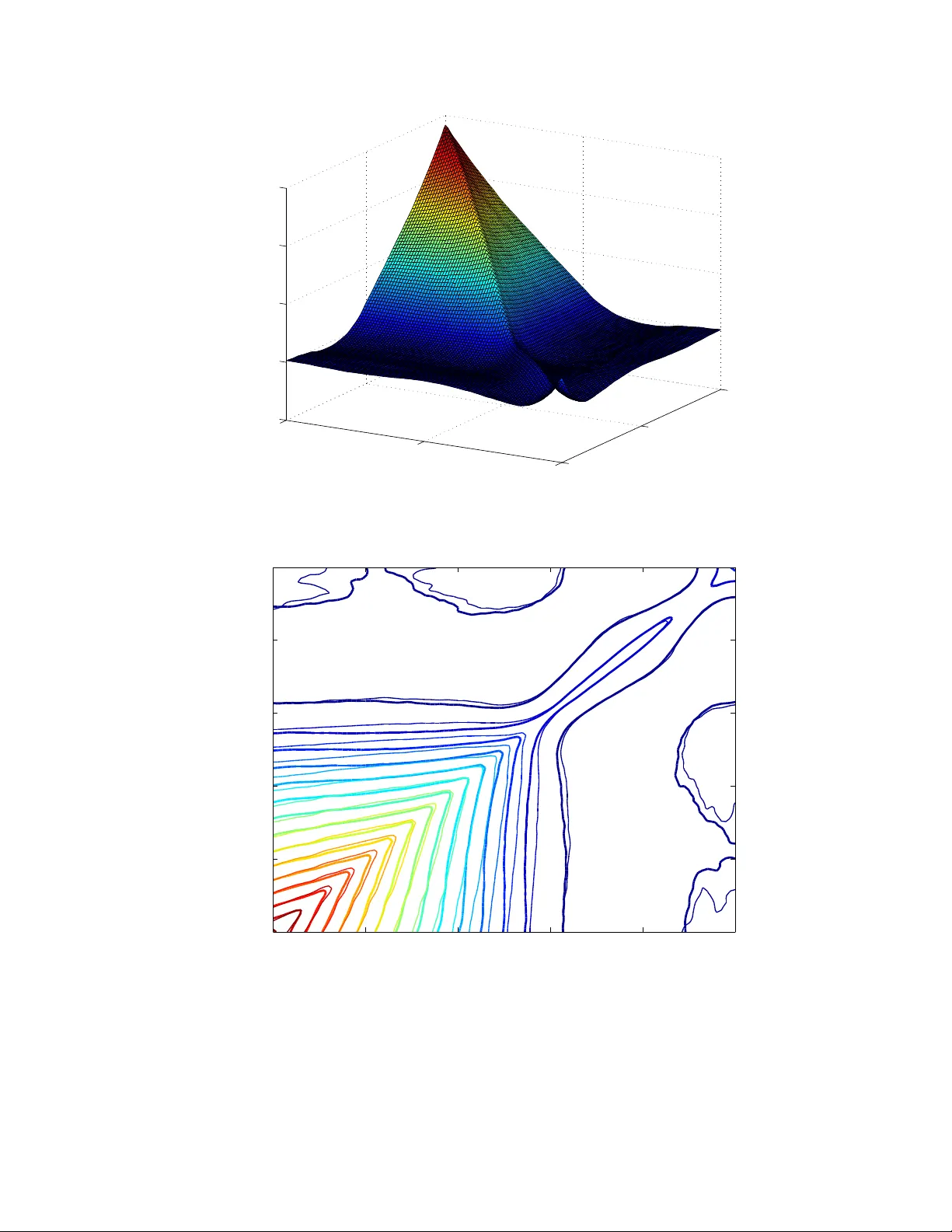
Ba y esian Inference with Optimal Maps T arek A. El Moselh y , Y oussef M. Marzouk Massachusetts Institute of T e chnolo gy, Cambridge, MA 02139, USA Abstract W e presen t a new approac h to Bay esian inference that en tirely a voids Mark ov c hain sim ulation, b y constructing a map that pushes forwar d the prior measure to the p osterior measure. Existence and uniqueness of a suitable measure-preserving map is established b y form ulating the problem in the con text of optimal transp ort theory . W e discus s v arious means of explicitly parameterizing the map and com- puting it eﬃciently through solution of an optimization problem, exploiting gradient information from the forward mo del when p ossible. The resulting algorithm ov er- comes man y of the computational b ottlenecks associated with Marko v c hain Monte Carlo. A dv an tages of a map-based representation of the p osterior include analytical expressions for p osterior momen ts and the ability to generate arbitrary n um b ers of indep enden t p osterior samples without additional likelihoo d ev aluations or forw ard solv es. The optimization approac h also pro vides clear con vergence criteria for p os- terior appro ximation and facilitates mo del selection through automatic ev aluation of the marginal lik eliho o d. W e demonstrate the accuracy and eﬃciency of the ap- proac h on nonlinear in v erse problems of v arying dimension, inv olving the inference of parameters app earing in ordinary and partial diﬀeren tial equations. Keywor ds: Ba yesian inference, optimal transp ort, measure-preserving maps, in verse problems, p olynomial chaos, numerical optimization 1. In tro duction The estimation of mo del parameters from observ ations is a ubiquitous problem in science and engineering. Inference or “in version” are central c hallenges in geoph ysics and atmospheric science, c hemical kinetics, quan titativ e biology , and a host of addi- tional domains. In all these settings, observ ational data ma y b e indirect, noisy , and limited in num ber or resolution. Quan tifying the resulting unc ertainty in parameters is then an essential part of the inference pro cess. Uncertaint y in mo del parameters in turn drives uncertaint y in predictions; c haracterizing the latter is vital to the use of Email addr esses: tmoselhy@mit.edu (T arek A. El Moselh y), ymarz@mit.edu (Y oussef M. Marzouk) Pr eprint submitte d to Journal of Computational Physics Novemb er 27, 2024 computational mo dels in design and decision-making, and even to subsequent rounds of data collection. The Bay esian statistical approach pro vides a foundation for learning from noisy and incomplete data, a natural mec hanism for incorp orating heterogeneous sources of information, and a complete assessmen t of uncertain ty in mo del predictions [ 1 – 5 ]. Uncertain quantities are treated as random v ariables, and the p osterior distribution, i.e., the probabilit y distribution of any quantit y of in terest (b e it a parameter or a mo del prediction) conditioned on data, represen ts one’s state of kno wledge ab out that quan tity . Characterizing the p osterior—sim ulating the distribution with samples; marginalizing; ev aluating moments, quan tiles, or credibilit y in terv als—th us becomes one of the cen tral computational challenges in Bay esian inference. In specialized cases (e.g., simple statistical mo dels with conjugate priors) exp ec- tations with resp ect to the p osterior may b e ev aluated in closed form. But in the general setting—and particularly when complex ph ysical mo dels en ter the lik eliho o d function—computational approac hes are needed. By far the most widespread and ver- satile metho d for p osterior simulation in this context is Marko v c hain Monte Carlo (MCMC) [ 2 , 6 – 10 ]. MCMC requires only p oin t wise ev aluations of an unnormalized densit y , and generates a stream of samples that can b e used to ev aluate p osterior exp ectations. Despite its p o wer and practical utility , MCMC suﬀers from man y limitations. Samples generated by the algorithm are necessarily correlated; strong correlation among successive samples leads to smaller eﬀectiv e sample sizes and larger errors in p osterior estimates [ 9 ]. An eﬃcien t MCMC algorithm endea vors to make the eﬀective sample size after N steps as close to N as p ossible, as the p osterior ev aluation(s) required at eac h step may be costly . Eﬃcient sampling in Metropolis-Hastings MCMC [ 8 ] rests on the design of eﬀectiv e pr op osal distributions , but this task is diﬃcult for target distributions that contain strong correlations or lo calized structure, particularly in high dimensions. Improv ements to MCMC prop osal mec hanisms are therefore the sub ject of in tense curren t in terest. A non-exhaustive list of recen t metho dological adv ances includes adaptivity based on past samples [ 11 , 12 ], Langevin metho ds [ 13 , 14 ], the use of Hessian information [ 15 ] and Hessians with low-rank structure [ 16 ], Hamiltonian dynamics [ 17 ], the exc hange of information among multiple c hains [ 18 – 20 ], multi-stage prop osals incorp orating approximate mo dels [ 21 , 22 ], and the use of surrogate or reduced mo dels to accelerate lik eliho o d ev aluations [ 23 – 27 ]. Ev en with these adv ances, MCMC remains a computationally in tensiv e pro cess; t ypical problems require many thousands or even millions of p osterior ev aluations. Moreo ver, the sampling pro cess do es not come with a clear conv ergence criterion, indicating when the c hain has adequately explored the distribution or how many ini- tial samples to discard as “burn-in.” Conv ergence diagnostics for MCMC are largely heuristic and remain something of an art [ 28 ]. Finally , the nature of MCMC is to represen t the p osterior distribution with samples; this may seem an obvious remark, but a sample represen tation immediately fav ors the use of Mon te Carlo metho ds 2 for subsequent uncertaint y propagation steps. F or computationally in tensive mo d- els, ho wev er, sampling may be impractical. More eﬃcien t uncertaint y propagation metho ds already exist [ 29 – 31 ] and it would be desirable to use them. Ev en sequential Mon te Carlo metho ds [ 32 ], designed with recursive inference and forecasting in mind, still rely on a w eighted-sample representation of the p osterior. In this pap er, we presen t a nov el approach to Ba yesian inference that relies on the construction of maps . W e entirely av oid Mark ov c hain simulation, and instead explic- itly construct a map that pushes forwar d the prior measure to the p osterior measure. In other w ords, the map transforms a random v ariable X , distributed according to the prior, in to a random v ariable Z , distributed according to the p osterior. Existence and uniqueness of a monotone map is assured under rather w eak conditions [ 33 ]. The map is actually found through solution of an optimization problem, which requires only the ability to ev aluate the p osterior density up to a normalizing constan t (exactly as in Metrop olis-Hastings MCMC). If gradien ts of the lik eliho o d function or forw ard mo del are av ailable, how ev er, then w e immediately take adv antage of them. T o make the optimization problem ﬁnite dimensional, the map is describ ed by multiv ariate orthogonal p olynomials; it therefore b ecomes a p olynomial c haos expansion [ 29 , 34 ] of the p osterior. As a byproduct of the optimization pro cedure, the scheme automatically calculates the p osterior normalizing constant, i.e., the marginal likelihoo d or evidence, which is an essen tial quan tit y in Ba y esian mo del selection [ 35 ]. W e sho w that the optimization pro cedure also pro vides an unambiguous con vergence criterion, with a quan tity that can b e monitored in order to decide whether to terminate iterations or to enrich the p olynomial space used to describ e the map. With a map in hand, one can c heaply generate indep endent p osterior samples b y simulating from the prior. Also, as the map is represented b y p olynomials orthogonal with resp ect to standard measures, p osterior momen ts may b e ev aluated algebraically . T o place the map-based sc heme in con text, we note that v ariational Ba yesian metho ds [ 36 ] also con vert inference in to an optimization problem, b y approximat- ing the p osterior with a simpler distribution from a parameterized family , p erhaps also chosen to ha v e a particular conditional indep endence structure. These are ap- pro ximations of the p osterior (or p osterior predictive) distribution function, how ev er. Distributions m ust b e chosen from particular families to facilitate optimization and sampling—in con trast to the presen t sc heme, which appro ximates random v ariables directly . The presen t sc heme has closer links to implicit ﬁltering metho ds [ 37 , 38 ] for sequen tial data assimilation. These metho ds rely on a weigh ted-sample represen- tation of eac h probabilit y distribution, but use maps to transp ort particles to high- probabilit y regions of the p osterior. Implicit ﬁltering eﬀectiv ely uses many maps, though, one for each particle and assimilation step. Unlike the present scheme, maps are not constructed explicitly; rather one ev aluates the action of eac h map on a single particle. The role of optimal transp ort in data assimilation has also b een raised in 3 [ 39 ]. This pap er is organized as follo ws: In Section 2 w e presen t the basic form ulation and sev eral alternativ e versions of the optimization problem that yields the map (Sec- tions 2.3 and 2.4 ). Metho ds for solving these optimization problems are presented in Section 3 . Section 4 presents a range of n umerical results. First, w e demonstrate our inferen tial approac h on a linear problem where the p osterior has kno wn analyt- ical form (Section 4.1 ). Then we p erform parameter inference in sev eral nonlinear ODE systems with strongly non-Gaussian p osteriors, and where the p osterior dif- fers markedly from the prior (Sections 4.2 and 4.3 ). Finally , w e demonstrate the approac h on high-dimensional in verse problems in volving the estimation of spatially heterogeneous co eﬃcien ts in elliptic PDEs (Section 4.4 ). 2. F orm ulation 2.1. Bayesian fr amework W e b egin b y describing the Bay esian inference framework and setting notation for the subsequen t developmen ts. Consider the task of inferring mo del parameters x from observ ations d . F or simplicit y , we will let b oth the parameters and observ ations b e real-v alued and ﬁnite-dimensional. In the Bay esian setting, the parameters and observ ations are treated as random v ariables. Let (Ω , F , P ) b e a probabilit y space, where Ω is a sample space, F is a σ -ﬁeld, and P is a probability measure on (Ω , F ) . Then the mo del parameters X : Ω → R n are asso ciated with a prior measure µ 0 on R n , such that µ 0 ( A ) = P ( X − 1 ( A )) for A ∈ R n . W e then deﬁne p ( x ) = dµ 0 /dx to b e the density of X with resp ect to Leb esgue measure. F or the presen t purp oses, w e assume that suc h a density alwa ys exists. W e then deﬁne the exp ectation with resp ect to the prior measure as E [ g ( X )] = R g ( x ) dµ 0 ( x ) = R g ( x ) p ( x ) dx , for any Borel-measurable function g on R n . The observ ational data are describ ed b y a random v ariable d taking v alues in R m . Inference requires that we deﬁne a probabilistic mo del for the data; in terms of probability densities, this mo del is simply p ( d | x ) . Viewed as a function of x , this conditional density deﬁnes the likeliho o d function L ( x ; d ) ≡ p ( d | x ) . Ba yes’ rule then yields the p osterior probabilit y density q ( x ) ≡ p ( x | d ) : q ( x ) = L ( x ; d ) p ( x ) β (1) where β is the evidence or marginal lik eliho o d β = R L ( x ; d ) p ( x ) dx . This posterior densit y q is associated with a posterior measure µ on R n , suc h that dµ ( z ) = q ( z ) dz and the lik eliho o d function is prop ortional to the Radon-Nik o dym deriv ative of µ with resp ect to µ 0 , L ( z ) ∝ dµ/dµ 0 [ 1 ]. In in verse problems [ 1 , 3 , 40 ], the likelihoo d frequen tly incorp orates a deterministic function h mapping the parameters to some idealized observ ations. This function h : R n → R m is termed the forwar d mo del . The discrepancy b etw een the idealized mo del predictions and the actual data is often assumed to b e additive: d = h ( x ) + ε , 4 where ε is a random v ariable. A common further assumption is that ε is Gaussian, zero-mean, and indep endent of the model parameters, i.e., ε ∼ N (0 , Σ) , leading to the follo wing form for the likelihoo d function: L ( x ; d ) = 1 (2 π ) m/ 2 (det Σ) 1 / 2 exp  − 1 2 k h ( x ) − d k 2 Σ  (2) where k u k A := k A − 1 2 u k , for an y p ositive symmetric matrix A . While the Ba yesian form ulation of inv erse problems commonly leads to likelihoo d functions that tak e the form of ( 2 ), w e emphasize that this particular form is not an assumption or requiremen t of the map-based inference metho d describ ed b elow. 2.2. Infer enc e with a map The core idea of our approach is to ﬁnd a map that pushes forward the prior measure to the posterior measure. In other words, supp ose that X is a random v ariable distributed according to the prior and that Z is a random v ariable distributed according to the p osterior. Then we seek a map f : R n → R n that satisﬁes the follo wing constraint, where equality is in distribution : Z = f ( X ) , with X ∼ µ 0 , Z ∼ µ. (3) Equiv alen tly , we seek a map f whic h pushes forward µ 0 to µ , i.e., for whic h µ = f ] µ 0 . A schematic of suc h a map is giv en in Figure 1 . The map necessarily dep ends on the data and the form of the lik eliho o d function. (In the case of ( 2 ), the map would thus dep end on the data d , the forward mo del h , and the distribution of the observ ational noise ε .) If the p osterior distribution w ere equal to the prior distribution, an identit y map would suﬃce; otherwise more complicated functions are necessary . Note that, for clarit y , we adhere to the strict association of a random v ariable with a distribu- tion. Th us the prior and p osterior distributions are asso ciated with distinct random v ariables ( X and Z , resp ectively) represen ting distinct states of kno wledge ab out the same set of parameters. This view is sligh tly diﬀerent than the usual notion of a single random v ariable for whic h we “up date” our b elief. Assuming that a map satisfying ( 3 ) exists and is monotone, 1 the measure of Z , represen ted b y the p osterior probability densit y q , can b e transformed in to a proba- bilit y density ˜ p for the input random v ariable X : ˜ p ( x ) = q ( f ( x )) | det D x f | = L ( f ( x ); d ) p ( f ( x )) β | det D x f | (4) where D x f = ∂ f /∂ x is the Jacobian of the map. But w e already ha ve a densit y for X , namely the prior density p . This in turn deﬁnes an alternate criterion for 1 A monotone (n on-decreasing) map f ( x ) on R n is one for which ( x 2 − x 1 ) T ( f ( x 2 ) − f ( x 1 )) ≥ 0 for every pair of distinct p oints x 1 , x 2 ∈ R n . Issues of existence and monotonicity will b e addressed in the next tw o subsections. 5 an inferen tial map: the transformed densit y ˜ p should b e equal to p , as depicted in Figure 2 : ˜ p ( x ) = p ( x ) . (5) The Ba yesian inference problem can thus b e cast in the following equiv alent form: Problem 2.1. Find a monotone map f ( x ) such that 2 [ L ◦ f ] ( x ) [ p ◦ f ] ( x ) β | det D x f | = p ( x ) . (6) In man y cases (e.g., when the lik eliho o d function and the prior density contain exp onen tials) the following expression is more appropriate for computation than ( 6 ): log ( L ◦ f ) + log ( p ◦ f ) − log β + log | det D x f | − log p = 0 . (7) W e emphasize that despite the app earance of the p osterior normalizing constant β in the problem ab ov e, our ﬁnal form ulation will nev er require kno wledge of β . Indeed, the v alue of β will emerge as a by-product of identifying the map. Instead of aiming for exact equality in ( 6 ), w e will deﬁne an optimization problem that seeks to minimize the discrepancy betw een the prior density p and the approx- imate and map-dep endent prior density ˜ p . This discrepancy can b e expressed, for instance, as the Kullbac k-Leibler div ergence or the Hellinger distance from p to ˜ p . W e will b egin by rewriting these discrepancies in a more conv enient form. F or the Hellinger distance Q ( p, ˜ p ) we hav e: Q ( p, ˜ p ) = 1 2 Z  p p ( x ) − p ˜ p ( x )  2 dx = 1 2 Z p ( x ) + ˜ p ( x ) − 2 p p ( x ) ˜ p ( x ) dx = Z 1 − p p ( x ) ˜ p ( x ) dx = 1 − Z p ( x ) s ˜ p ( x ) p ( x ) dx = 1 − E " s ˜ p ( X ) p ( X ) # . (8) Similarly , the Kullback-Leibler (KL) div ergence from p to ˜ p can be rewritten as fol- lo ws: D KL ( p || ˜ p ) = Z p ( x ) log p ( x ) ˜ p ( x ) dx = − E  log ˜ p ( X ) p ( X )  . (9) 2 T o simplify notation we use [ L ◦ f ]( x ) to denote L ( f ( x )) . W e also drop the explicit dep endence of L on the data d . 6 Both the square ro ot in ( 8 ) and the log in ( 9 ) are conca ve functions Φ , and Jensen’s inequalit y provides that E  Φ  ˜ p p  ≤ Φ  E  ˜ p p  . (10) T o minimize either Hellinger distance ( 8 ) or KL d iv ergence ( 9 ) we w ould therefore like to ac hieve equality ab ov e, but equalit y holds if and only if the ratio ˜ p/p is constant in x [ 41 ]. Consisten t with ( 6 ), the v alue of this constant should be unity . Re-arranging equation ( 4 ), w e obtain the following expression for β β = [ L ◦ f ] ( x ) [ p ◦ f ] ( x ) p ( x ) | det D x f | . (11) T aking the logarithm of this expression w e obtain T ( x ; f ) := log ( L ◦ f ) + log ( p ◦ f ) + log | det D x f | − log p = log β . (12) Equation ( 12 ) is the cornerstone of our analysis. It states that T ( x ; f ) should b e constan t o v er the supp ort of the prior. Setting T to b e a constan t suggests the follo wing problem formulation: Problem 2.2. Find f ∗ ( x ) such that f ∗ = arg min f V ar [ T ( X ; f )] (13) wher e X ∼ µ 0 . Note that this form ulation is equiv alen t to minimizing either of the discrepancy measures b etw een ˜ p and p considered ab o ve (and others as w ell). Moreo ver, if f is allo wed to lie within a suﬃciently ric h function space, we kno w exactly what minim um v alue of V ar [ T ] can b e attained: zero. As emphasized earlier, f ∗ is computed without an y kno wledge of the evidence β , since the latter do es not appear in T . Ho w ever, β can b e ev aluated as β = exp ( E [ T ( X )]) . (14) An alternativ e optimization problem can obtained by observing that D KL ( p || ˜ p ) = − E  log ˜ p ( X ) p ( X )  = log β − E [ T ( X )] . Since log β is a constan t, minimizing D KL ( p || ˜ p ) is equiv alent to seeking: f ∗ = arg max f E [ T ( X ; f )] . (15) In other w ords, w e maximize the numerical estimate of the evidence. Unlike Prob- lem 2.2 , this formulation do es not hav e a known optimal v alue of the ob jective func- tion, but V ar[ T ] can nonetheless b e monitored to assess conv ergence. 7 2.3. The optimal tr ansp ort formulation The m ultiv ariate map f : R n → R n tak es the following general form: z i = f i ( x 1 , x 2 , . . . , x n ) , i = 1 . . . n (16) where f i are the comp onen ts of f . Using the classic measure transform literature [ 33 , 42 – 45 ] one can sho w that a map pushing µ 0 forw ard to µ exists under relatively w eak conditions, but is not unique. T o guaran tee uniqueness, extra constraints or p enalties m ust b e enforced. T w o types of constraints are employ ed in this pap er. The ﬁrst, discussed in this section, is an optimal transp ort constrain t. It can b e sho wn [ 33 ], under remark ably general conditions, that the optimization problem min f E  k X − f ( X ) k 2  sub ject to µ = f ] µ 0 (17) has a unique solution f ∗ and that this solution is monotone . Conditions for existence and uniqueness essen tially require that the measure µ 0 (here, the prior) not contain an y atoms. W e restate this result more precisely as follows: Theorem 2.3. (After [ 33 , 45 ]) L et µ 0 and µ b e Bor el pr ob ability me asur es on R n with µ 0 vanishing on subsets of R n having Hausdorﬀ dimension less than or e qual to n − 1 . Then t he optimization pr oblem ( 17 ) has a solution f that is uniquely determine d µ 0 - almost everywher e. This map is the gr adient of a c onvex function and is ther efor e monotone. F or a detailed pro of of this theorem see, e.g., [ 45 ]. T o b e sure, our true ob jective is not to ﬁnd th e optimal transp ort of Theorem 2.3 p er se. Instead we w ant to add enough regularit y to Problem 2.2 such that w e can ﬁnd a monotone map satisfying f ] µ 0 ≈ µ (or equiv alen tly ˜ p ≈ p ). T o this end, we use the optimal transp ort problem ( 17 ) to motiv ate the follo wing p enalized ob jectiv e: min f  D KL ( p || ˜ p ) + λ E  k X − f ( X ) k 2  . (18) By analogy with Problem 2.2 , ( 18 ) can b e replaced b y: Problem 2.4. Find f to solve the fol lowing optimization pr oblem min f  V ar [ T ( X )] + λ E  k X − f ( X ) k 2  . (19) Equations ( 18 ) and ( 19 ) should b e understo o d as follo ws. The ﬁrst term en- forces the measure transformation from prior to posterior, 3 while the second term is 3 See App endix A for a discussion of the relativ e magnitudes of V ar[ T ] and the KL div ergence. 8 a p enalt y inspired by the optimal transp ort form ulation to promote regularit y and monotonicit y in f . The magnitude of the p enalty term is controlled by the multiplier λ . In the optimization scheme to b e detailed in Section 3 , this m ultiplier is c hosen adaptiv ely , suc h that the magnitude of the p enalty term is a prescrib ed fraction (e.g., 1 / 10 ) of the magnitude of V ar [ T ] or D KL ( p || ˜ p ) at the start of each cycle. The stop- ping criterion for the optimization scheme ev aluates only the ﬁrst term of ( 18 ) or ( 19 ), since this is the term that enforces the accuracy of the p osterior represen tation. W e also emphasize that in every example tested b elow (see Section 4 ), the v alue of λ w as not a critical parameter in the optimization pro cedure. In fact λ can b e assigned a zero v alue when V ar [ T ( X )] is suﬃciently small. One could also, of course, rev ert to solving the constrained optimization prob- lem ( 17 ) and th us ﬁnd the true L 2 -optimal transp ort. W e do not pursue suc h a sc heme here, ho wev er, b ecause our core in terest is in satisfying the measure transfor- mation condition, not in ﬁnding the optimal transp ort p er se. 2.4. T riangular formulation An alternativ e method for guaran teeing a unique solution is to enforce a “trian- gular” structure for the map. Th is construction is inspired b y the Rosen blatt trans- formation [ 46 , 47 ], where now the i th comp onent of f can dep end only on the ﬁrst i inputs: z i = f i ( x 1 , . . . , x i ) . (20) In this form ulation, the regularity of the problem is provided by the triangular structure and no additional p enalt y term is required to ensure uniqueness. Indeed, [ 48 ] sho ws that there exists a unique monotone map f of the form ( 20 ) satisfying µ = f ] µ 0 . 4 This map is kno wn as the Knothe-Rosenblatt re-arrangement [ 45 , 48 ]. The Rosen blatt re-arrangement is typically computed via an iterativ e pro cedure [ 45 ] that in volv es ev aluating and inv erting a series of marginalized conditional cu- m ulative distribution functions. This pro cedure is computationally v ery intensiv e, since it in v olves computing a large num b er of high-dimensional in tegrals. Instead of explicitly computing the Rosenblatt transformation in this wa y , w e propose to solve the follo wing problem: Problem 2.5. Find f ∗ = arg min f V ar [ T ( X )] , (21) wher e f is subje ct to the structur e ( 20 ). One could mo dify the optimization problem b y replacing V ar [ T ( X )] with D KL ( p || ˜ p ) in ( 21 ). W e thus prop ose to ﬁnd a Rosen blatt-type re-arrangement all-at-once rather 4 This result [ 48 ] places conditions on µ 0 essen tially requiring that the marginals of µ 0 ha ve no atoms. A suﬃcient condition is that µ 0 b e absolutely contin uous with resp ect to Leb esgue measure. Also, just as in Theorem 2.3 , uniqueness of the map holds µ 0 -almost everywhere. 9 than comp onent by comp onen t, and with a stopping criterion that inv olv es the mag- nitude of the entire ob jectiv e function b eing smaller than a prescrib ed threshold. W e must ackno wledge, ho w ever, that the curren t theory [ 48 ] do es not preclude the existence of non-monotone measure-preserving maps that hav e the triangular struc- ture. Th us the question of whether minimizing V ar [ T ( X )] sub ject to ( 20 ) guar ante es monotonicit y of the map remains open. In n umerical tests on a wide v ariet y of in- ference problems, how ever, the solutions w e obtain using the triangular constrain t are consisten tly monotone. Monotonicit y is easily v eriﬁed b y examining det D x f ; it should ha ve the same sign ( µ 0 -a.e.) ov er the supp ort of the prior. Note that one can exploit the triangular structure in order to express the deter- minan t of the Jacobian of the map as a pro duct of the diagonal terms: det D x f = det ∂ f ∂ x = n Y i =1 ∂ f i ( x 1 , . . . , x i ) ∂ x i . (22) 3. Solution Algorithm Problem 2.4 and its triangular v ariant are sto chastic optimization problems, in that they inv olv e exp ectations with resp ect to the prior distribution. They are also inﬁnite-dimensional, in that f (in principle) may b e an element of an inﬁnite- dimensional function space. Moreov er, they ma y in volv e lik eliho o d functions L that are deﬁned implicitly through the solution of forw ard p roblems h and that are com- putationally intensiv e. W e will describ e algorithms for the solution of these problems, taking into account all of the ab o ve c hallenges. The algorithms inv olve sample ap- pro ximations of the prior expectation, a ﬂexible p arameterization of f , and eﬃcien t gradien t-based optimization. Later w e describ e a con tinuation-t yp e metho d for solv- ing a sequence of simpler optimization problems to yield a “cascade” or sequence of maps. 3.1. Monte Carlo sampling It is in general complicated or imp ossible to compute momen ts of T ( X ) using analytical formulae. Instead, we use Monte Carlo sampling to approximate the ex- p ectation op erator E [ T ( X )] ≈ 1 N s N s X i =1 T  x ( i )  (23) where x ( i ) ∼ µ 0 . Notice that the exp ectation is taken with respect to the prior, whic h is assumed to b e a distribution from which one can easily generate indep endent samples. (Extensions to the metho d ma y address situations where prior sampling is diﬃcult; see Section 5 .) The num b er of samples N s is c hosen adaptively ov er the course of the optimization algorithm, as describ ed in Section 3.4 . Moreo ver, the set x ( i ) is “refreshed” with a new batch of i.i.d. samples b etw een cycles. In this sense, the presen t sc heme b ears strong similarities to the SAA (sample a v erage appro ximation) approac h to sto chastic programming [ 49 ]. 10 3.2. Polynomial appr oximation of f As noted ab o ve, the optimization problems p osed in Section 2.3 and 2.4 are inﬁnite-dimensional. T o make them more computationally feasible, the map f ( x ) is appro ximated using a ﬁnite set of basis functions. In a high dimensional infer- ence problem, the use of lo calized basis functions is in general not eﬃcien t; instead, a global basis is more suitable. In our implemen tation, we represen t f using mul- tiv ariate p olynomials orthogonal with resp ect to the prior measure; in other w ords, w e write the map as a p olynomial chaos expansion [ 29 , 30 , 34 , 50 ]. Some additional in tuition for p olynomial maps is as follo ws. An identit y map f : R n → R n yields a p osterior that is equal to the prior. An aﬃne map containing a diagonal linear transformation, i.e., where f i dep ends only on x i , allows changes of lo cation and scale in each comp onent of the parameter v ector, from prior to p osterior, but preserves the form of each distribution. An aﬃne map con taining a general linear transformation (with eac h f i dep ending on all comp onen ts of x ) allo ws the in tro duction of new cor- relations in the p osterior. Quadratic, cubic, and higher-degree maps allo w ev en more complex distributional c hanges from prior to p osterior. W e write the p olynomial expansion of f as: f ( x ) = X i ∈J g i ψ i ( x ) (24) where i = ( i 1 , i 2 , ..., i n ) ∈ N n is a m ulti-index, g i ∈ R n are the expansion co eﬃcien ts, and ψ i are n -v ariate p olynomials. W e write each of these p olynomials as ψ i ( x ) = n Y j =1 ϕ i j ( x j ) (25) where ϕ i j is a univ ariate p olynomial of order i j in the v ariable x j , orthogonal with resp ect to the distribution of x j . F or simplicity , w e assume here that the prior can b e describ ed, p erhaps after some transformation, by a set of indep enden t random v ari- ables. That said, orthogonal polynomial expansions for dep endent random v ariables with arbitrary probability measure can certainly b e constructed [ 51 ]. The set of multi- indices J describ es the truncation of the expansion. F or example J = { i : | i | 1 ≤ n 0 } corresp onds to a total-order expansion of degree n 0 , con taining K = card ( J ) =  n + n 0 n 0  = ( n + n 0 )! n ! n 0 ! (26) terms. The orthogonal p olynomial representation of the map oﬀers several adv antages, b esides b eing con venien t and ﬂexible (b y c hoice of J ). First, moments of the p oste- rior distribution—i.e., moments of f ( X ) , with X ∼ µ 0 —can b e ev aluated analytically , without the need for further sampling or additional forward mo del solv es. F or exam- ple, the posterior co v ariance is a weigh ted sum of outer products of the coeﬃcients: 11 Co v ( Z ) = P i g i g T i E [ ψ 2 i ] . Higher momen ts can be ev aluated using kno wn formulas for the expectations of pro ducts of orthogonal polynomials [ 30 , 52 ]. Second, obtain- ing a p olynomial c haos expansion of the p osterior facilitates eﬃcient propagation of data-conditioned uncertaint y through subsequen t computational mo dels. This is a k ey step in p osterior prediction and in sequen tial data assimilation (e.g., ﬁltering). With a p olynomial c haos represen tation in hand, a v ast arra y of stochastic Galerkin and sto c hastic collo cation metho ds can b e emplo yed for uncertaint y propagation. T reating eac h co eﬃcient g i ∈ R n as a column v ector, we assemble the set { g i } i ∈J in to a matrix F T of size n × K , where K denotes card ( J ) : F T =  g 1 g 2 . . . g K  . (27) In the optimal transp ort form ulation all n × K co eﬃcients are considered the opti- mization v ariables, whereas in the triangular formulation some of these co eﬃcients are ﬁxed to zero. The map f is then then represented as f ( x ) = F T Ψ( x ) (28) where Ψ( x ) is a column v ector con taining every basis p olynomial ψ i , i ∈ J . 3.3. Newton ’s metho d and nonline ar le ast squar es In our implemen tation w e use tw o alternative algorithms to solve the optimization problem: Newton’s metho d and nonlinear least squares. In the standard Newton’s metho d, we compute b oth the ﬁrst and second deriv atives of the ob jective function. It is then necessary to compute the deriv atives of T ( x ) with resp ect to the optimization v ariables F : T ( x ; F ) = log ( L ◦ f ) + log ( p ◦ f ) + log | det D x f | − log p ∂ T ∂ F =  1 L ◦ f dL ( f ) d f + 1 p ◦ f dp ( f ) d f  ∂ f ∂ F + D x Ψ ( D x f ) − 1 where ∂ f /∂ F = [ I n ⊗ Ψ( z )] . The last term is obtained as follo ws: D x f = D x  F T Ψ  = F T D x Ψ ∂ ∂ F ij (log | det D x f | ) = trace(( D x f ) − 1 E j i D x Ψ) = trace(( D x f ) − 1 e j [ D x Ψ] ( i, :)) = [ D x Ψ] ( i, :) ( D x f ) − 1 e j ∂ ∂ F (log | det D x f | ) = D x Ψ ( D x f ) − 1 (29) where E j i is a matrix of all zeros except for a single 1 at the location ( j, i ) and e j is a v ector of zeros except for a 1 in ro w j . 12 The second deriv ativ es of T can b e obtained in a similar fashion. In the case of a Gaussian prior and Gaussian additiv e noise, explicit expressions for the ﬁrst and second deriv atives are given in Appendix C . Note that to compute any deriv atives of the likelihoo d function, deriv ativ es of the forw ard mo del are required. Using mo dern adjoin t techniques, gradients and Hessian-vector pro ducts can typically b e computed at the cost of O (1) forw ard solves, indep endent of the dimension of the parameter space [ 16 ]. In man y problems, ho wev er, the forward mo del and its deriv ativ es can b e accurately appro ximated using surrogate mo dels [ 24 ]. The second deriv ativ es of the log-determinant can b e calculated explicitly as: ∂ 2 ∂ F ∂ F ij (log | det D x f | ) = − D x Ψ ( D x f ) − 1 ( E j i D x Ψ) ( D x f ) − 1 = − D x Ψ ( D x f ) − 1 ( e j [ D x Ψ] ( i, :)) ( D x f ) − 1 = −  D x Ψ ( D x f ) − 1 e j   [ D x Ψ] ( i, :) ( D x f ) − 1  . (30) F rom the previous relations it is clear that in order to compute the Hessian of the log-determinan t, w e must ﬁrst compute the matrix D x Ψ ( D x f ) − 1 and then use the outer pro duct of appropriate column and ro w vectors to assem ble the desired Hessian. Alternativ ely , one can use a nonlinear least squares (NLS) metho d to solve the problem. This metho d is particularly suited to the triangular formulation of Sec- tion 2.4 , whic h do es not hav e a p enalty term. T o cast the optimization ob jectiv e as a nonlinear least squares problem, it is observ ed that the zero v ariance condition V ar [ T ( X )] = 0 is equiv alen t to T  x ( i )  = constan t, for x ( i ) ∼ p . In other words, T is constan t in an L 2 sense. This leads to the set of equations T  x ( i ) ; F  = 1 N s N s X j =1 T  x ( j ) ; F  . (31) If the num b er of optimization parameters ` < nK in F is less than N s , then ( 31 ) is an o verdetermined set of nonlinear equations in F , whic h can b e solved via M ∆ F = b F k +1 = F k − ∆ F (32) where the rectangular matrix M ∈ R N s × ` and the column v ector b ∈ R N s are: M ( i, :) = ∂ T  x ( i )  ∂ F − 1 N s N s X j =1 ∂ T  x ( j )  ∂ F b ( i ) = T  x ( i ) ; F  − 1 N s N s X j =1 T  x ( j )  . (33) Here, the deriv ative of a scalar with resp ect to a vector is assumed to b e a row v ector. 13 W e ha ve observed that in certain cases, e.g., weakly multi-modal p osteriors, con- v ergence of the algorithm from arbitrary initial maps is more reliable if the ob jectiv e function is mo diﬁed to b ecome min f  V ar [ T ( X )] + λ E   T ( X ) − ˜ β  2  , (34) where ˜ β is an estimate of the evidence computed from the previous iteration. In this case, the nonlinear least squares formulation pro ceeds from the following s et of equations: T  x ( i ) ; F  = 1 1 + λ 1 N s N s X j =1 T  x ( j ) ; F  + λ ˜ β ! , i = 1 . . . N s . (35) In general, w e initialize our algorithm using the identit y map, f ( x ) = x . Alter- nativ ely , if the likelihoo d contains additive Gaussian noise and the prior is Gaussian, w e linearize the forward mo del and compute the resulting map analytically . This appro ximate linear map is then used to initialize the algorithm. 3.4. A lgorithm structur e W e solv e the optimization problem in stages, b y iterating ov er the order of the p olynomial represen tation of f ( x ) . W e typically start the algorithm with only linear basis functions in Ψ( x ) . After computing the best linear map, the total order of the p olynomial basis is increased and a new corresp onding map is computed—allowing co eﬃcien ts of al l the polynomial terms to b e adjusted, not just those of the highest degree. This pro cess is rep eated un til reac hing a stopping criterion V ar [ T ( X )] < δ , where δ is a preset threshold. The samples used to approximate the prior exp ectation or v ariance are renewed eac h time the order of the expansion is increased. The num b er of samples N s is c hosen suc h that approximations of the mean or v ariance obtained with successive sample batc hes lie within some predetermined relativ e tolerance α of eac h other, typically 5%. Algorithm 1 summarizes our complete approach. Notice that the m ultiplier λ is used only when computing the penalized map of Problem 2.4 . The v alue of this m ultiplier is adjusted each time the order of the expansion is increased; it is c hosen suc h that the p enalty term is 10% of the total v alue of the ob jectiv e function at the start of the current stage. Th us λ decreases as f con verges tow ards the desired measure transformation. 3.5. Comp osite map In certain problems, the map from prior to p osterior can b e accurately appro xi- mated only with v ery high-degree polynomials. Unfortunately , the n um b er of co eﬃ- cien ts in a m ultiv ariate p olynomial expansion gro ws very rapidly with degree, leading to a more c hallenging optimization problem. 14 Algorithm 1: Structure of optimization algorithm for computing the map. Data : Likelihoo d function L , observ ed data, prior densit y p , stopping criterion δ , sample tolerance α Result : Map f ( x ) f ( x ) = x , i = 0 , and λ = 1 ; n 0 = 1 ; while V ar [ T ( X )] > δ do i = i + 1; Generate N s i.i.d. samples of the prior random v ariable; if i > 1 then Compute V ar[ T ( X )] ; if | (V ar[ T ( X )] /V ∗ ) − 1 | > α then Double the n umber of samples N s ← 2 N s ; end end Solv e the optimization problem for f ( x ) up to desired order n 0 , stopping when ∆ F is smaller than a threshold; Get curren t V ar[ T ( X )] and store it in V ∗ = V ar[ T ( X )] ; Increase order of expansion: n 0 ← n 0 + 2 ; If applicable compute a new λ = 0 . 1 V ∗ / E [ k X − f ( X ) k 2 ] end T o o vercome this diﬃcult y , w e can use a c omp osition of maps to eﬃcien tly ap- pro ximate a high-degree transformation from prior to p osterior. That is, instead of mapping the prior to the p osterior with a single map, we introduce a sequence of in termediate distributions that evolv e gradually from prior to p osterior. With this sequence of distributions, we introduce a corresp onding sequence of maps. In tuitively , this approach “relaxes” the measure transformation problem; if the input and output distributions are similar to each other, then the presumably the map can b e well appro ximated using lo w-degree p olynomials. Letting the n umber of steps approach inﬁnit y , one could imagine a con tinuous transformation from prior to p osterior, for instance as prop osed in [ 39 ]. Here w e focus on ﬁnite sequences of intermediate distributions. There are man y w ays that one could create such a sequence: iterating ov er the accuracy of the forward mo del, gradually in tro ducing comp onents of the data vector d , or iterating o ver the scale of the noise cov ariance in the lik eliho o d function. W e c ho ose the latter tactic, b eginning with a large co v ariance Σ 1 and in tro ducing k stages suc h that the v ariance of the last stage is the true Σ of the original inference problem: Σ 1 > Σ 2 > · · · > Σ k = Σ (36) 15 F or a giv en noise v ariance Σ i , a comp osite map φ i ≡ f i ◦ f i − 1 ◦ · · · ◦ f 1 (37) is computed suc h that it maps the prior distribution µ 0 (with densit y p ) to the inter- me diate posterior distribution µ i (with densit y q i ) corresp onding to i th-stage noise lev el. Then we can minimize, e.g., min F i D KL  p ||  q i ◦ φ i    det D x φ i    (38) with a regularization term added abov e as needed. Here only the parameters F i of the i th map f i are optimization v ariables! Coeﬃcients of the preceding maps are ﬁxed, having b een determined in the previous stages’ optimization problems. See Figure 3 for a schematic. The resulting map f = φ k ≡ f k ◦ f k − 1 ◦ · · · ◦ f 1 will ha ve b een computed with signiﬁcantly less eﬀort (and few er degrees of freedom) than a total-order p olynomial of the same maxim um degree. One adv antage of the sequential construction ab o ve is that the accuracy of an in termediate map, transforming the prior to any of the intermediate distributions q i , do es not aﬀect the accuracy of the ﬁnal map. Because the prior densit y p alwa ys app ears in ( 38 ), the ﬁnal stage can b e b e computed with tight error tolerances to yield the appropriate measure transformation. In termediate maps ma y b e computed with lo oser tolerances, as they serve in a sense only to ﬁnd distributions that are closer in shap e to the actual p osterior. Any error in an intermediate f can b e comp ensated for b y the ﬁnal f k . In our implemen tation, we hav e observed that this sc heme is robust and that it allo ws for simple error con trol. Alternativ ely , one could think of computing the map one stage at a time—i.e., at eac h step computing a transformation f i from q i − 1 to q i b y minimizing min F i D KL  q i − 1 ||  q i ◦ f i    det D x f i    . (39) The ﬁnal map is again f = φ k ≡ f k ◦ f k − 1 ◦ · · · ◦ f 1 . A p ossible adv antage of this second construction is that one needs to consider only a single map at a time. Eac h stage m ust b e solv ed exactly , ho wev er, as the construction dep ends on satisfying µ i = φ i ] µ 0 for all i . If φ i do es not push forw ard µ 0 to µ i , then an y error incurred in the ﬁrst i stages of the sequence will remain and corrupt the ﬁnal stage. Also, b ecause the error tolerances in the in termediate stages cannot b e relaxed, the diﬃculty of computing an y of the intermediate maps could conceiv ably b e as great as that of computing the full map. F or these reasons, we prefer the ﬁrst construction ( 38 ) and will use it when demonstrating comp osite maps in the n umerical examples (Section 4.3 ) b elow. 4. Results W e no w demonstrate map-based inference on a series of example problems, ranging from parameter estimation in linear-Gaussian mo dels (allowing v eriﬁcation against a kno wn analytical solution) to nonlinear ODEs and high-dimensional PDEs. 16 4.1. Line ar-Gaussian mo del Here w e demonstrate the accuracy and con vergence of our method on ov er- and under-determined linear-Gaussian mo dels. W e ev aluate b oth the optimal transp ort form ulation and the triangular formulation. Consider a linear forward mo del h ( x ) = Ax , where the parameters x are endow ed with a Gaussian prior, x ∼ N (0 , Σ P ) , and additiv e measuremen t noise ε yields the data: d = h ( x ) + ε = Ax + ε . (40) If the noise is further assumed to b e Gaussian, ε ∼ N (0 , Σ N ) , then the p osterior is Gaussian, and the map f is linear and a v ailable in closed form: f ( x ) = z 0 + Z 1 x (41) with Z 1 Σ P Z T 1 = Σ post =  A T Σ − 1 N A + Σ − 1 P  − 1 z 0 = µ post = Σ A T Σ − 1 N d. (42) In addition, the evidence can b e computed in closed form: β = exp  − 1 2  d T Σ − 1 N d − µ T post Σ − 1 post µ post   p | det Σ N | . (43) A detailed deriv ation of the previous relations is giv en in App endix B . W e ﬁrst test the t wo optimization form ulations (the p enalized optimal transp ort ob jectiv e of Section 2.3 and the triangular construction of Section 2.4 ) on an o ver- determined inference problem with 10 parameters and 16 observ ations. The forward mo del, represented b y A ∈ R 16 × 10 , is randomly generated with en tries of A inde- p enden tly sampled from a standard normal distribution. W e use an identit y prior co v ariance Σ P = I and put Σ N = σ 2 I with σ = 0 . 06 . With b oth formulations (Problem 2.4 and Problem 2.5 ), w e observ e con v ergence to a map matching ( 42 ) after 15 iterations. The evidence β also con verges to its analytical v alue, to within machine precision. With the optimal transp ort formula- tion, w e observ e that our Z 1 diﬀers from the symmetric matrix square ro ot of the p osterior cov ariance b y roughly 5%. More precisely , the F rob enius norm k · k F of the diﬀerence, k Z 1 − Σ 1 / 2 post k F , is roughly 5% of k Σ 1 / 2 post k F . When the triangular construc- tion is emplo y ed, the F rob enius norm of Z 1 − L is less than 10 − 6 k L k F , where L is the low er-triangular Cholesky factor of Σ post , i.e., Σ post = LL T . With the optimal transp ort formulation, w e ha ve further observ ed that if the map f is forced to remain symmetric and if the p enalt y factor λ is gradually reduced to zero, then Z 1 matc hes Σ 1 / 2 post with a relativ e error of less than 10 − 6 . Next w e consider a larger but under-determined linear-Gaussian problem with 100 parameters and 8 observ ations, again randomly generating A . Using the triangular 17 construction, w e compute the map. Con vergence plots of V ar [ T ] and the Kullbac k- Leibler divergence D KL ( p || ˜ p ) are given in Figure 4 , while conv ergence of the evidence β is shown in Figure 5 . The optimization iterations b egin with the iden tity map, and the v ariance and KL divergence decrease rapidly to zero as the correct map is iden tiﬁed. (Note that KL divergence is not sho wn in the ﬁrst ﬁve iterations of Figure 4 , because the sample-estimated div ergence is inﬁnit y .) Near conv ergence, it is observ ed that the v alue of the Kullbac k-Leibler divergence is approximately half the v ariance of T ( X ) . This relation is pro ven in App endix A . 4.2. R e action kinetics This example demonstrates map-based inference on a nonlinear problem that yields a non-Gaussian p osterior, with a sharp lo wer b ound and strong correlations. The problem is t wo-dimensional, enabling direct visualization of the map. W e exam- ine the impact of truncating the polynomial order on conv ergence and monotonicit y of the map. The ob jective of the problem is to infer the forward and rev erse rates of reaction in the chemical system A k 1  k 2 B [ 11 ]. The go verning equations are as follows, with u represen ting the concen tration of comp onent A and v the concen tration of comp onent B : du dt = − k 1 u + k 2 v dv dt = k 1 u − k 2 v . (44) The initial condition is ﬁxed at u (0) = 1 and v (0) = 0 . The rate parameters k 1 and k 2 are endo wed with indep endent Gaussian prior distributions, k 1 ∼ N (2 , 200 2 ) and k 2 ∼ N (4 , 200 2 ) . The “true” parameter v alues are set to k 1 = 2 , k 2 = 4 , and synthetic data consisting of noisy observ ations of u at times t = 2 , 4, 5, 8, and 10 are generated. Observ ational noise is assumed to b e i.i.d. Gaussian. Because the observ ations o ccur relativ ely late in the dynamics of the ODE initial v alue problem, the only information whic h can b e inferred is the ratio of k 1 and k 2 —i.e., the equilibrium constan t of the system. W e compute a map using the algorithm detailed in Section 3 . The map is rep- resen ted using a total-order polynomial expansion. W e begin with a linear map and progressiv ely increase its order; at the end of iterations with a 5th-order map ( n 0 = 5 ), the Kullbac k-Leibler div ergence D KL ( p || ˜ p ) is less than 10 − 3 . The algorithm requires a total of 30 inner-lo op optimization steps to reac h this level of accuracy . Figure 6 shows 10 4 samples from b oth the prior and p osterior distributions. As exp ected, the p osterior samples concentrate around the line k 2 = 2 k 1 . Also, p osterior samples are lo calized in the upp er left quadrant of the k 1 - k 2 plane, which corresp onds to stable tra jectories of the ODE. In b oth Figures 6(a) and 6(b) , sample p oin ts at whic h the determinan t of the Jacobian D x f is negativ e are sho wn in red. Elsewhere 18 (blue p oints), the Jacobian determinant is p ositiv e. This sign c hange corresp ond s to regions of the parameter space where monotonicit y of the map is lost; w e note that all of these p oin ts are relegated to the tails of the prior distribution. Only 0.08% of the samples ha ve negative determinant. Figures 7(a) and 7(b) sho w comp onents of the map itself, via surface plots of f 1 ( k 1 , k 2 ) and f 2 ( k 1 , k 2 ) . The tw o comp onen ts of the map are nearly identical up to a scaling factor of t wo, which is to be exp ected, as the p osterior distribution contains a strong correlation b et ween the parameters. 4.3. Genetic to ggle switch In this example we demonstrate the comp osite map on a six-dimensional nonlinear parameter inference problem using real exp erimental data. W e compare the accuracy of our results to those obtained with a standard MCMC algorithm. The example in volv es the dynamics of a genetic “toggle switc h” [ 53 ]. The toggle switc h consists of tw o repressible promotors arranged in a mutually inhibitory net- w ork: promoter 1 transcrib es a repressor for promoter 2, while promoter 2 transcrib es a repressor for promoter 1. Either repressor ma y b e induced b y an external c hemical or thermal signal. Genetic circuits of this form ha ve b een implemented on E. c oli plasmids, and the follo wing ODE mo del has b een prop osed [ 53 ]: du dt = α 1 1 + v β − u dv dt = α 2 1 + w γ − v w = u  1 + [IPTG] κ  − η (45) Here u is the concen tration of the ﬁrst repressor and v is the concentration of the second repressor. [IPTG] is the concen tration of IPTG, the chemical comp ound that induces the switc h. At low v alues of [IPTG] , the switch is in the ‘low’ state, reﬂected in low v alues of v ; con v ersely , high v alues of [IPTG] lead to strong expression of v . As in [ 54 ], w e w ould like to infer the six mo del parameters α 1 , α 2 , β , γ , η and κ . T o this end, we emplo y actual experimental data 5 consisting of normalized steady-state v alues of v at selected IPTG concentrations, spanning the ‘lo w’ and ‘high’ sides of the switc h: [IPTG] ∈ { 10 − 3 , 0 . 6 , 1 , 3 , 6 , 10 } × 10 − 3 . 5 Data are courtesy of Dr. T. S. Gardner. 19 A t steady state, the mo del yields the following relations u = α 1 1 + v β v = α 2 1 + w γ w = u  1 + [IPTG] κ  − η whic h can b e expressed as an implicit function v = g ( v , ξ ) , where ξ = ( α 1 , α 2 , β , γ , η , κ ) . The elements of ξ are endow ed with indep enden t uniform prior distributions, centered at the nominal v alues ξ 0 suggested in [ 53 ]: ξ 0 =  156 . 25 , 15 . 6 , 2 . 5 , 1 , 2 . 0015 , 2 . 9618 × 10 − 5  . In other w ords, we hav e ξ i = ξ 0 ,i (1 + σ i θ i ) (46) where θ is a v ector of uniformly-distribu ted random v ariables, θ i ∼ U ( − 1 , 1) , and en tries of σ are (0 . 20 , 0 . 15 , 0 . 15 , 0 . 15 , 0 . 30 , 0 . 20) . As detailed in [ 54 ], the observ ational error is assumed Gaussian and zero-mean, with a standard deviation that dep ends on whether the expression level is lo w or high. This simpliﬁed error mo del is consisten t with exp erimen tal observ ations. The use of uniform priors adds an extra constraint on the map: since the prior supp ort is a unit h yp ercube (with appropriate scaling), the range of the map must b e an improp er subset of the unit h yp ercub e, just as the supp ort of the p osterior is con tained within the supp ort of the prior. This constraint is diﬃcult to satisfy when the map is approximated using global p olynomials. T o circum ven t this diﬃculty , w e ﬁrst map the uniform random v ariables θ to independent standard normal random v ariables x ∼ N (0 , I ) using the error function: θ = erf  x/ √ 2  ∼ U ( − 1 , 1) (47) Computation of the map can now pro ceed using a Gaussian prior on the input x . After computing the map f ( x ) , the p osterior random v ariable ξ post is obtained through the same transformation: ξ post = ξ 0 h 1 + σ erf  f ( x ) / √ 2 i (48) All deriv atives of ξ with respect to x are computed analytically using ( 46 ) and ( 47 ), e.g., dξ dx = ξ 0 σ √ 2 π exp  − x 2 2  . (49) 20 Using the implicit expression for v , we can compute the deriv atives of v with resp ect to an y mo del parameter ξ i : ∂ v ∂ ξ i = ∂ g ∂ ξ i + ∂ g ∂ v ∂ v dξ i ∂ v ∂ ξ i = ∂ g ∂ ξ i  1 − ∂ g ∂ v  − 1 . (50) The second deriv ativ es are: ∂ 2 v ∂ ξ i ξ j = ∂ g 2 ∂ ξ i ∂ ξ j + ∂ 2 g ∂ ξ i ∂ v ∂ v ∂ ξ j +  ∂ 2 g ∂ v 2 ∂ v dξ j + ∂ 2 g ∂ v ∂ ξ j  ∂ v ∂ ξ i + ∂ g ∂ v ∂ 2 v ∂ ξ i ∂ ξ j ∂ 2 v ∂ ξ i ξ j =  1 − ∂ g ∂ v  − 1  ∂ 2 g ∂ ξ i ∂ ξ j + ∂ 2 g ∂ ξ i ∂ v ∂ v ∂ ξ j +  ∂ 2 g ∂ v 2 ∂ v dξ j + ∂ 2 g ∂ v ∂ ξ j  ∂ v ∂ ξ i  . (51) T o compute deriv ativ es with resp ect to the transformed Gaussian random v ariables x , the c hain rule is applied: ∂ v ∂ x = ∂ v ∂ ξ dξ dx ∂ 2 v ∂ x 2 = ∂ v ∂ ξ d 2 ξ dx 2 +  dξ dx  T ∂ 2 v ∂ ξ 2 dξ dx . With these transformations in place, we turn to the n umerical results in Figures 8 – 10 . In this problem, a high-order map is required to accurately capture the p osterior distribution, and thus w e employ the c omp osite map of Section 3.5 . In particular, w e compute the o verall map using a four-stage cascade of third order maps, f = f 1 ◦ · · · ◦ f 4 . The distributions obtained after each stage are shown in Figures 8(a) – 8(d) , using a scatter plot of output samples from eac h map ( φ 1 , φ 2 , etc). While the p osterior is six-dimensional, these plots fo cus on the pairwise marginal distribution of α 1 and γ ; this is the most “complex” pairwise marginal and is particularly sensitive to the accuracy of f . These distributions are shown on the transformed Gaussian domain, and th us they corresp ond to the ﬁrst and fourth comp onents of x : x α 1 and x γ . F or comparison, Figure 8(e) sho ws results obtained using a long run of delay ed- rejection adaptiv e Metrop olis (DRAM) MCMC [ 11 ], with 10 6 samples. In Figures 9(a) – 9(f ) w e sho w the marginal p osterior probability densit y of eac h comp onen t of ξ , obtained at the end of the four-map sequence. These densities are compared with densities obtained using the long MCMC run; the map-based results sho w go o d agreemen t with the latter. Figure 10 sho ws samples from the join t prior of x α 1 and x α 2 . As sp eciﬁed abov e, these parameters are indep endent and standard normal. The p oint of this ﬁgure is not the distribution p er se, but rather the color lab eling, which diagnoses the monotonicity of the map. The map is ev aluated on 10 6 samples from the prior. Among these samples, only 861 hav e Jacobian determinants that are negative; all the rest are p ositive. As in the previous example, the few samples with negativ e Jacobian determinan t are concen trated in the tails of the distribution. A w ay from the tails, the map is monotone. 21 4.4. PDE-c onstr aine d inverse pr oblems Examples in this section focus on high-dimensional inv erse problems inv olving partial diﬀeren tial equations (PDEs). In particular, our ob jective is to estimate a spatially heterogeneous co eﬃcient κ app earing in an elliptic PDE, from noisy and lim- ited observ ations of the solution ﬁeld [ 55 ]. W e solv e the problem on one-dimensional (Section 4.4.1 ) and t wo-dimensional (Section 4.4.2 ) spatial domains. W e employ the triangular parameterization of the map, p erforming quantitativ e comparisons of com- putational eﬃciency and accuracy with MCMC for a range of data sets and observ a- tional noise magnitudes. 4.4.1. One-dimensional domain Consider a linear elliptic PDE on the unit in terv al S = [0 , 1] ∇ · ( κ ( s ) ∇ u ) = − f ( s ) (52) where s ∈ S is the spatial co ordinate, ∇ ≡ ∂ /∂ s , and f is a known source term. In the subsurface context, this equation describ es Darcy ﬂow through p orous media, where κ represen ts a p ermeabilit y ﬁeld and u is the pressure. W e apply b oundary conditions ∂ u ∂ s   s =0 = 0 and u | s =1 = 1 . The source term is given by: f ( s ) = a exp  − 1 2 b 2 ( s − s m ) 2  (53) with a = 100 , s m = 0 . 5 , and b = 0 . 01 . W e place a log-normal prior on the p ermeabilit y ﬁeld κ , log [ κ ( s, ω ) − κ 0 ] ∼ G P (0 , C ) (54) and let the co v ariance kernel c ( s, s 0 ) of the Gaussian pro cess ha ve exp onential form c ( s, s 0 ) = σ 2 exp  − | s − s 0 | L c  . (55) 6 W e use a prior standard deviation of σ = 1 . 5 and a correlation length L c = 0 . 5 , along with an oﬀset κ 0 = 0 . 5 . Realizations of this spatial process are rough; in fact, they are not mean-square diﬀeren tiable. 6 Note that c ( s, s 0 ) is the Green’s function of the diﬀeren tial op erator − L c 2 σ 2 d 2 ds 2 + 1 2 σ 2 L c (56) with appropriate b oundary conditions [ 56 , 57 ]. Hence the inv erse cov ariance op erator C − 1 is explic- itly represented by ( 56 ). 22 The problem is spatially discretized using ﬁnite diﬀerences on a uniform grid, with spacing ∆ s = 1 / 100 . The log-normal p ermeabilit y ﬁeld is sto chastically discretized using the Karh unen-Lo ève expansion of the underlying Gaussian pro cess: log [ κ ( s, ω ) − κ 0 ] ≈ n X i =1 φ i ( s ) p λ i x i ( ω ) (57) where x i ∼ N (0 , 1) are indep enden t standard normal random v ariables, and φ i , λ i are the eigenfunctions and eigenv alues of the linear op erator corresp onding to the co v ariance k ernel: R S c ( s, s 0 ) φ i ( s ) ds = λ i φ ( s 0 ) . W e discretize the eigenfunctions on the same grid used to discretize the PDE solution ﬁeld u . T o capture 99% of the spatially-in tegrated v ariance of the log-normal pro cess, we retain n = 66 Karh unen- Lo èv e mo des. Noisy observ ations of u are obtained at m p oints in space. The noise is additiv e and i.i.d. Gaussian, such that d j = u ( s j ; x ) + ε j with ε j ∼ N (0 , σ 2 n ) , j = 1 . . . m . The observ ational data is generated by c ho osing a “true” p ermeability ﬁeld κ , solving the ful l PDE mo del ( 52 ) to obtain the corresp onding pressure ﬁeld u ( s ) , then corrupting u ( s ) at the m measuremen t lo cations with indep enden t realizations of the noise. In the inference pro cess, on the other hand, w e use the p olynomial chaos expansion ( 58 ) as the forw ard mo del. This discrepancy ensures that w e do not commit an “in verse crime” [ 3 ]. An y Ba y esian inference strategy , whether the map-based optimization approach or MCMC, requires rep eated ev aluations of the forw ard mo del. As suggested in [ 24 ], exploiting regularity in the dep endence of u on the parameters x can mak e these ev aluations more computationally tractable. W e therefore approximate u ( s ; x ) using a polynomial chaos expansion. W e apply the iterativ e algorithm dev elop ed in [ 58 ], for the solution of high-dimens ional sto chastic PDEs, to obtain an appro ximation of u in the form: u ( s ; x ) = X k ∈K u k ( s ) ψ k ( x ) (58) where u k are co eﬃcien ts and ψ k ( x ) are m ultiv ariate Hermite p olynomials, c hosen adaptiv ely within a very large basis set K . Algorithm 1 allo ws the expansion order of the map f ( x ) to b e increased in stages; i.e., w e b egin by ﬁnding a linear map, then a cubic map, and so on. Since infer- ence problems in v olving distributed parameters are typically high-dimensional (in the current problem f maps R 66 on to itself, for example), writing f as a total-order p olynomial expansion in all n of its comp onents will lead to a very large num b er of de- grees of freedom, most of which are not needed to ac hieve an accurate representation of the posterior. Instead, we reﬁne the p olynomial description of the map in a more ﬁnely-grained fashion. Recall that f ( x ) = F T Ψ( x ) , where Ψ is a v ector of orthogonal p olynomials in x 1 . . . x n . In the structure of Algorithm 1 , decisions to expand the p olynomial description of the map are made outside of the inner optimization lo op, 23 after chec king whether V ar[ T ] satisﬁes the desired threshold δ . Now, rather than rais- ing the polynomial degree of the en tire map (e.g., n 0 ← n 0 + 2 ), w e c ho ose a subset of the inputs { x i : i ∈ I } and introduce higher-degree p olynomial terms in these v ariables only . The index set I initially consists of { 1 , 2 , . . . , i 1 < n } . A t the next iteration, if the v ariance threshold is still not satisﬁed, i 1 is replaced with a larger index i 2 , where i 1 < i 2 < n . This pro cess contin ues un til the largest elemen t in I is n or until V ar[ T ] stagnates. No w I is reset and new p olynomial terms of ev en higher degree, in volving only x 1 through x i 1 , are added to the expansion. Then the index set is expanded once again. In any of these iterations, adding terms to the expansion is equiv alen t to adding rows to Ψ( x ) and to the matrix of p olynomial co eﬃcients F . T o make this pro cess more concrete, consider what happens in the present infer- ence problems. W e b egin by solving for the p olynomial co eﬃcien ts of a linear map (p ossibly sub ject to the triangular constraint). The optimal linear map is not able to reduce V ar[ T ] b elow the requisite threshold. P olynomial terms of total order n 0 = 3 in the ﬁrst i 1 = 10 (for example) comp onents of x are then introduced, and all the co eﬃcien ts collected in F are adjusted via optimization. This reﬁnement of f is still not suﬃcien t, so now the order-3 expansion is extended to the ﬁrst i 2 = 20 (again for example) comp onen ts of x . Extension to additional comp onents of x is observ ed to yield little decrease in the minimal v alue of V ar[ T ] , so no w the p olynomial space is enric hed b y adding terms of total order n 0 = 5 in the ﬁrst i 1 comp onen ts of x . Iter- ations con tinue un til conv ergence, resulting an “adapted” map f whose components are a subset of a total-order expansion in x 1 . . . x n . Results of our algorithm are shown in Figures 11 – 13 , where we also rep ort com- parisons with MCMC. W e consider three cases, corresp onding to diﬀerent num b ers of observ ations m and diﬀeren t noise levels σ 2 n . In Case I, w e hav e m = 31 observ ations and a noise standard deviation of σ n = 0 . 05 ; in Case I I, w e increase the n umber of data p oints to m = 101 and retain σ n = 0 . 05 ; in Case I I I w e k eep m = 101 observ a- tions and reduce the noise standard deviation to σ n = 0 . 01 . In all cases, the maximum p olynomial order of th e map is 5 and the optimization routine is terminated when V ar[ T ] < δ = 0 . 1 . W e use the triangular form ulation and a single map (rather than a comp osite map) for these problems. Figures 11(a) – 11(f ) plot the p osterior mean and standard deviation of the log- p ermeabilit y ﬁeld as computed with optimal maps and with MCMC. The “truth” log-p ermeabilit y ﬁeld, used to generate the data, is sho wn in black. As exp ected in this ill-conditioned problem, only the smo oth part of the p ermeabilit y ﬁeld can b e reconstructed. As the n umber of data p oin ts increases and the noise lev el decreases, ho wev er, more features of the p ermeabilit y ﬁeld can b e reco vered. The posterior co v ariance is non-stationary , and we note that the p osterior v ariance is m uc h smaller at the righ t b oundary , where there is a Diric hlet b oundary condition, than at the left boundary , where a zero Neumann condition was imp osed. Ov erall, p osterior uncertain ty decreases from Case I to Case I I I, reﬂecting additional information in the data. Go o d agreement b et w een the map and MCMC results is observed, though 24 MCMC yields a sligh tly larger standard deviation in the left half of the domain. The curren t MCMC results w ere obtained using 10 6 samples of DRAM, with the ﬁrst 5 × 10 5 samples discarded as burn-in. Simple MCMC conv ergence diagnostics suggest that this is an adequate n um b er of samples, but it is not en tirely clear whic h set of results is more authoritative. Indeed, we observed that DRAM failed to conv erge in almost half the attempted runs of Case I I I. (These runs w ere initiated from the prior mean; diﬀerences among the attempted runs result from randomness in the prop osals.) On the other hand, the optimal map algorithm reliably conv erges to the desired tolerance δ . Figure 12 shows p osterior realizations for Case I and Case II I, as computed with the map and with MCMC. Note that the realizations are diﬀerent in c haracter than the p osterior mean; they are signiﬁcantly rougher, as one would exp ect given the exp onen tial cov ariance kernel in the Gaussian pro cess prior. But the map and MCMC results yield p osterior realizations of similar c haracter. In Figure 13 we plot the p osterior co v ariance of log ( κ − κ 0 ) from Case I. W e c ho ose this case b ecause of the apparen t discrepancy in p osterior standard deviations shown in Figure 11(b) . Figure 13(a) is a surface plot of the p osterior cov ariance as computed using our map algorithm. The exp onen tial prior cov ariance has a discon tinuit y in its deriv ativ e at the diagonal, smo othed sligh tly due to truncation at a ﬁnite num b er of Karh unen-Lo ève mo des. This feature is preserved in the posterior, reﬂecting the fact that p osterior realizations are also rough and that data are not informativ e at the smallest scales. The o v erall scale of the co v ariance is reduced signiﬁcantly from prior to posterior, how ever. While the prior cov ariance was stationary with σ 2 = 1 . 5 , the p osterior sho ws smaller v ariance throughout the spatial domain. In Figure 13(b) we compare the con tours of p osterior co v ariance obtained with the map to those obtained using MCMC algorithm. The 16 contour levels range uniformly from − 0 . 1 to 1.4. Contours computed using the tw o metho ds are remark ably similar. It should be emphasized that ﬁnding the map f enables the p osterior co v ariance to b e computed analytically . 4.4.2. Two-dimensional domain T o explore the p erformance of our algorithm in a more challenging setting, w e solv e the same inv erse problem as in Section 4.4.1 but on a t w o-dimensional spatial domain S = [0 , 1] 2 . The gov erning equation is still ( 52 ), but no w s ≡ ( s 1 , s 2 ) ∈ S and ∇ ≡ ( ∂ /∂ s 1 , ∂ /∂ s 2 ) . W e apply deterministic Diric hlet b oundary conditions on all four sides of S , with u (0 , 0) = 0 , u (0 , 1) = 1 , u (1 , 1) = − 1 , u (1 , 0) = 2 and a linear v ariation on ∂ S b et w een these corners. The source term f is of the form ( 53 ), cen tered at s m = (0 . 5 , 0 . 5) and with width b = √ 10 / 40 . The equation is discretized on a 41 × 41 grid. Again w e place a l og-normal prior on the p ermeability ﬁeld ( 54 ) with κ 0 = 1 , c ho osing an isotropic exp onential co v ariance k ernel c ( s, s 0 ) with σ = 1 . 25 and L c = 0 . 5 . T o capture 95% of the spatially integrated v ariance of the prior p ermeability 25 ﬁeld, the next t wo cases employ n = 39 Karhunen-Loève mo des. T w o diﬀeren t data conﬁgurations are considered. The ﬁrst (Case A) uses m = 121 observ ations randomly scattered on the spatial domain, with noise standard deviation σ n = 0 . 08 ; the second (Case B) inv olv es m = 234 randomly scattered observ ations and noise standard deviation σ n = 0 . 04 . As in the one-dimensional problem, a p olynomial c haos approximation of u ( s, x ) is used as the forw ard mo del for inv ersion. W e ﬁrst fo cus our analysis on the p osterior distribution of the Karhunen-Loève mo de w eights { z i } , where z = f ( x ) and x i ∼ N (0 , 1) . Figure 14(a) shows a boxplot of the mo de weigh ts computed using the map. The exten t of each blue b o x marks the 25% and 75% quan tiles of the p osterior marginal of each z i , while the vertical lines or “whiskers” span the entire range of the posterior samples dra wn via the map. W e also plot the p osterior mean of z i obtained with the map (circle) and with MCMC (an × ). Finally we sho w the mo de weigh ts corresp onding to the “true” p ermeabilit y ﬁeld used to generate the data, b efore the addition of observ ational noise. The map and MCMC means agree reasonably well. Comparing the results of inference with the true weigh ts, it is observ ed that the ﬁrst few mo des are accurately iden tiﬁed, whereas the higher-index mo des are not. This is b ecause the higher-index mo des are rougher; they corresp ond to higher-frequency comp onents of the p ermeability ﬁeld, whic h are smo othed by the elliptic op erator and therefore diﬃcult to iden tify from observ ations of u . This trend is further demonstrated b y Figure 14(b) , which sho ws the p osterior standard deviation of eac h mode, computed with the map and with MCMC. As the mo de indices increase, their p osterior v ariances approac h unity—whic h is exactly the prior v ariance on x i . Thus the data con tained little information to constrain the v ariabilit y of these mo des. T urning from analysis of the Karh unen-Lo èv e mo des to analysis of the p ermeabil- it y ﬁeld itself, Figure 15 sho ws the truth log-p ermeability ﬁeld used to generate the data (which here reﬂects truncation to n = 39 Karhunen-Loève mo des). Figure 16(a) sho ws the p osterior mean log-p ermeability obtained with the map in Case A. Giv en the smo othing character of the forward mo del, the presence of noise on the data, and mismatc h b et ween the full PDE model used to generate the noiseless data and the PC appro ximation used for in version, w e should not expect the p osterior mean and the true p ermeability ﬁeld to matc h exactly . Indeed, the p osterior mean matches the true ﬁeld in its large-scale behavior, but most of the lo calized or small-scale features are lost; the corresp onding mo de w eights necessarily revert to their prior mean of zero. Figure 16(b) shows the p osterior standard deviation of the log-p ermeabilit y as computed with the map, while Figures 17(a) and 17(b) sho w the p osterior mean and standard deviation ﬁelds computed with MCMC. Results obtained via the t wo algo- rithms are v ery similar. The computational time required to solv e the optimization problem for the map, with tolerance δ = 0 . 5 , is equal to the time required for 5 × 10 5 steps of MCMC. Figures 18 – 20 show analogous results for Case B, with roughly t wice as man y ob- serv ations and half the noise standard deviation of Case A. The b oxplot of Karhunen- 26 Lo èv e (KL) mo de w eights in Figure 18(a) sho ws that a larger n umber of mo des (at higher index) are accurately identiﬁed, compared to Case A. In Figure 18(b) , the p osterior standard deviation of the mo des is less than in Case A, reﬂecting the ad- ditional information carried b y the data. Figure 19(a) sho ws the posterior mean log-p ermeabilit y obtained with the map for Case B; though this ﬁeld is still smo oth, more of the small-scale features of the true permeability ﬁeld are captured. MCMC results sho wn in Figure 20 are quite similar to those obtained with the map. The MCMC results rep orted here were obtained using a DRAM c hain of 10 6 samples, half of which were discarded as burn-in. W e make no claim that this is most eﬃcien t MCMC approach to this problem; certainly a carefully hand-tuned algorithm could yield b etter mixing. Ho wev er, w e do claim that it represents go o d MCMC p erformance. Because the inference problem has b een transformed to the Karhunen- Lo èv e mo des, which ha ve unit v ariance and are uncorrelated in the prior, the adaptiv e Metrop olis algorithm starts from a fa vorable parameterization with kno wn scaling. Ev en with a goo d parameterization and an adaptiv e algorithm, ho wev er, MCMC mixing remains a c hallenge in these ill-p osed in verse problems. Figure 21 shows the eﬀectiv e sample size (ESS) of eac h comp onent of the c hain corresp onding to N = 5 × 10 5 p ost burn-in samples. The eﬀective sample size is computed by in tegrating the c hain auto correlation ρ i at lag i : ESS = N 1 + 2 P ∞ i =1 ρ i . (59) The ESS for most of the c hain comp onents lies b et w een 1500 and 4000. In order to obtain a reasonable num b er of p osterior samples—e.g., for an accurate estimate of a p osterior moment, or to propagate p osterior uncertaint y through a subsequen t sim ulation—an unreasonable n umber of MCMC steps is th us required. F or instance, if one desires 10 5 eﬀectiv ely indep endent posterior samples, then at least 30 million MCMC steps are needed (here, corresp onding to ab out 2 days of sim ulation time). On the same computational platform and for the same problem, using the map algorithm to generate 10 5 indep enden t samples requires ab out 45 min utes of wallclock time to solv e the optimization problem and construct f , follow ed b y 5 min utes to pass 10 5 prior samples through the map and generate the desired posterior samples. This corresp onds to a factor of 50 reduction in computational time. W e also note that when the noise standard deviation is reduced to σ n = 0 . 01 , then the adaptiv e MCMC algorithm fails to con verge, pro ducing a c hain with near-zero acceptance rate regardless of ho w many times we rerun it (starting from the prior mean). On the other hand, the map algorithm has no trouble conv erging to the desired accuracy δ in roughly 55 minutes of wallclock time (only 10 min utes more than that required for Case B). As a ﬁnal example we consider a more reﬁned sto chastic discretization of the prior log-normal pro cess. W e now retain n = 139 Karhunen-Loève mo des, such that 97.5% 27 of the input permeability ﬁeld’s integrated v ariance is preserv ed. W e mak e m = 227 noisy observ ations, with a noise standard deviation of σ n = 0 . 04 . In this example w e fo cus on comparing the computational p erformance of MCMC and map-based inference. T w o diﬀeren t MCMC chains are run, eac h of length 10 6 samples. Both c hains start from the prior mean and pro ceed with adaptiv e random-w alk prop osals. It is observ ed that the burn-in p erio d is relatively long; w e th us remov e half the chain and use the remaining 5 × 10 5 samples to compute all quan tities b elow. Each c hain tak es approx- imately 5 hours to produce. The map algorithm is run un til the v ariance of T ( X ) is less than 1% of the mean of T ( X ) ; this corresp onds to a KL divergence D KL ( p || ˜ p ) of 1 nat. The computational time required to solve the optimization problem to this threshold is less than 3 hours. Figure 22 sho ws the p osterior mean v alues of the Karh unen-Lo ève modes com- puted u sing MCMC and the map. The tw o MCMC runs sho wn in Figure 22(a) diﬀer signiﬁcan tly in their higher-index mo des, indicating that these comp onents of the c hain mix rather p o orly . Comparing the map-based p osterior means with the “truth” sho ws, as usual, that the smo other mo des are w ell iden tiﬁed in the p osterior while the rougher mo des are not, rev erting i nstead to the prior. P o or mixing of the MCMC algorithm is also evident in Figure 23 , which sho ws the p osterior standard deviation of eac h mo de weigh t. F or mo de indices larger than 10, the tw o MCMC runs yield v ery diﬀeren t standard deviations. And the standard deviations of the higher-index mo des plateau b elow 0.8. The discrepancy b et w een the chains suggests that this v alue is not credible, and that the chains are in fact not exploring the full parameter space (despite using 10 6 samples). One would instead exp ect the rough highest-index mo des to rev ert to the prior standard deviation of 1.0, exactly as observed in the map-based results. Indeed, agreemen t of the prior and p osterior distributions on the high-index KL mo des is a consequence of absolute contin uity of the posterior with resp ect to the prior [ 55 ]. Limitations of standard MCMC algorithms in this con text ha ve b een discussed in [ 59 ]. In Figure 24 w e compute eﬀectiv e sample sizes for one of the MCMC c hains from the previous ﬁgures. The minim um ESS o v er all c hain components is 275; the median, mean, and max ESS are 543, 561, 1100, resp ectively . Extrap olating these n umbers lets us determine the total computational (wallclock) time needed to compute an y n um b er of eﬀectiv ely independent samples via MCMC. Figure 25 th us compares the computational eﬀort of MCMC to that required by the map. W e neglect the computational time asso ciated with an y MCMC burn-in p eriod, eﬀectively giving MCMC a signiﬁcant b o ost in the p erformance comparison. The time required by the MCMC algorithm grows linearly with the num b er of indep enden t samples. On the other hand, the map requires a ﬁxed amoun t of time at the outset, in order to solv e the optimization problem, while the computational cost for each new sample p oin t is almost negligible. (The latter still grows linearly with the n umber of samples but with a very small slope.) Here, if one is in terested in generating few er than 300 28 indep enden t samples, then MCMC is faster; otherwise ﬁnding the optimal map is more eﬃcien t. Figure 26 shows a similar comparison, but uses the num b er of forward mo del ev al- uations as a measure of computational eﬀort, rather than wallclock time. W e assume that deriv atives of the forw ard mo del output with resp ect to the mo del parameters can b e computed with an adjoin t metho d, which means that the cost of computing the ﬁrst deriv atives is equiv alent to appro ximately tw o forward solv es. F urthermore, p er the current implemen tation, w e assume that second deriv atives of the forward mo del with resp ect to the parameters are not computed. In this comparison, the break-even p oin t is approximately 200 samples. If the desired num b er of samples is smaller, then MCMC is more eﬃcien t; otherwise the map algorithm can oﬀer order-of-magnitude reductions in computational eﬀort. Finally , w e note that all of the computations ab ov e ha ve used a serial implemen- tation of the map-based inference approach. It should b e emphasized, how ever, that the bulk of the computational eﬀort inv olved in solving the optimization problem for the map and subsequen tly generating samples is em barrassingly parallel. 5. Conclusions W e hav e presented a new approach to Ba yesian inference, based on the explicit construction of a map that pushes forwar d the prior measure to the p osterior measure. The approach is a signiﬁcan t departure from Mark ov chain metho ds that c haracter- ize the p osterior distribution by generating correlated samples. Instead, the present approac h ﬁnds a deterministic map f through the solution of an optimization pr ob- lem . Existence and uniqueness of a monotone measure-preserving map is established using results from optimal transp ort theory . W e adapt these results and prop ose tw o alternativ e optimization formulations, one with an explicit regularization term in the ob jectiv e and one that regularizes the problem by constraining the structure of f . The new form ulation oﬀers sev eral adv an tages o v er previous metho ds for Bay esian computation: • The optimization problem pro vides a clear conv ergence criterion, namely that V ar[ T ( X )] → 0 , with T ( X ) deﬁned in ( 12 ). Monitoring this criterion can be used to terminate iterations or to adaptiv ely enric h the function space used to describ e the map, un til a desired level of accuracy is reached. • The posterior normalizing constant, or evidence, is computed “for free” as an output of the optimization problem. • Because w e describ e the map using standard orthogonal p olynomials, p osterior momen ts may b e computed analytically from the p olynomial co eﬃcien ts. • Once a map is in hand, arbitrary num b ers of indep endent p osterior samples ma y b e generated with minimal computational cost, by applying the map to samples from the prior. 29 • While the optimization ob jectiv e inv olves prior exp ectations and is th us sto chas- tic, eﬃcient gradient-based metho ds (e.g., Newton or quasi-Newton metho ds, with the full mac hinery of adjoin ts) can nonetheless b e used to solv e the opti- mization problem. • A sequence of low-order maps ma y b e c omp ose d to capture the transition from prior to p osterior; this construction allo ws a complex c hange of measure to b e captured more economically than with a single map. W e demonstrate the map-based approac h on a range of examples. F ast conv ergence to the exact solution is observ ed in a linear parameter inference problem. W e also infer parameters in a nonlinear ODE system, u sing real exp erimen tal data, where the p osterior is of complicated form and diﬀers in shap e from the prior. Finally , w e use the map to tac kle several high-dimensional, ill-p osed, and nonlinear in verse problems, in volving inference of a spatially heterogeneous diﬀusion co eﬃcient in an elliptic PDE. Ov erall, inference with maps proceeds with greater reliability and eﬃciency than MCMC—particularly on high-dimensional in verse problems. Speedup can b e quan- tiﬁed in simple wa ys, suc h as coun ting the computational eﬀort required to pro duce a certain n umber of eﬀectively indep enden t p osterior samples. In the presen t prob- lems, the cost of computing the map with typical tolerances is equiv alent to obtaining roughly 200 indep endent samples with MCMC. But these comparisons are necessarily insuﬃcien t, b ecause inference with maps provides mor e information and more useful diagnostics than MCMC, as detailed ab o ve. Sev eral promising a ven ues exist for future w ork. There is ample opportunity to impro v e the eﬃciency of the optimization algorithms. First, w e note that each optimization step can b e made embarrassingly parallel, as it relies on prior sampling. Among the most computationally intensiv e elemen ts of the optimization pro cedure is the ev aluation of the forward mo del h , comp osed with the map, on each prior sample. P arallelizing these computations and their corresponding adjoint solv es w ould lead to immediate and substan tial computational gains. More eﬃcien t optimization approac hes ma y also employ imp ortance sampling to compute the v ariance or mean of T , or introduce sto chastic expansions for T itself. The map itself is a p olynomial chaos expansion of the p osterior distribution, and th us it is readily suited to propagation of p osterior uncertaint y through subsequen t dynamics. With this p osterior propagation step comes an immediate extension to recursiv e inference problems, i.e., ﬁltering and prediction with sequential data. More- o ver, in the presen t work, w e ha ve fo cused on measure transformations from prior to p osterior, but one could also create maps that push forward some third “base” measure to b oth the p osterior and prior. Suc h a construction could b e useful when it is not con venien t or easy to generate indep enden t prior samples, or if the prior is improp er. There are sev eral t yp es of static inference problem for whic h the map approac h m ust b e further developed. The examples presented in this pap er had only one ‘level’; 30 extensions of map-based inference to include hyperparameters, or more generally , to exploit the structure of Ba yesian hierarchical mo dels, are currently ongoing. Another c hallenge arises when the p osterior has b ounded supp ort, with signiﬁcant probability mass accum ulating near a b oundary . The range of the map must b e appropriately b ounded in suc h cases. Th us far w e ha v e circum v ented suc h problems b y reparame- terization, transforming b ounded domains in to un b ounded ones. This tric k comes at a computational price, e.g., greater nonlinearity . W e ask, then, how more directly to b ound the range of the map, whether on a b ounded or un b ounded input domain, via constrain ts in optimization or p erhaps a non-p olynomial basis. W e w ould also like to b etter understand the limiting behavior of the map in ill- p osed and high-dimensional problems. When inferring distributed parameters with some meaningful correlation structure—in the elliptic inv erse problem, for example— there is a natural ordering of the random v ariables and adaptive enric hment of the map works well. But in high-dimensional nonlinear problems with no natural order- ing (for instance, nonlinear ODE systems with h undreds of unkno wn parameters), a high-order p olynomial expansion in all the mo des is computationally prohibitiv e. F urther exploration of adaptive methods, perhaps coupled with dimensionality re- duction, is needed. W e ask, for example, whether inferential maps hav e a lo w-rank tensorial represen tation or a sparse represen tation in some basis. Finally , w e note that generating multi-modal p osterior distributions from unimo dal priors will require more lo calized structure in the maps than global p olynomial basis functions can feasi- bly provide. Piecewise p olynomials, multi-elemen t p olynomial chaos [ 60 ], and similar represen tations may b e quite useful in such problems. A c knowledgmen ts The authors would like to ac kno wledge supp ort from the US Departmen t of En- ergy , Oﬃce of Science, Oﬃce of A dv anced Scientiﬁc Computing Researc h (ASCR) under gran t num b ers DE-SC0002517 and DE-SC0003908. References [1] A. M. Stuart, In verse problems: a Ba yesian p ersp ective, A cta Numerica 19 (2010) 451–559. [2] A. Gelman, J. B. Carlin, H. S. Stern, D. B. Rubin, Bay esian Data Analysis, Chapman and Hall/CR C, 2nd edition, 2003. [3] J. Kaipio, E. Somersalo, Statistical and Computational Inv erse Problems, Springer, 2004. [4] D. S. Sivia, J. Skilling, Data Analysis: A Ba yesian T utorial, Oxford Science Publications, 2nd edition, 2006. 31 [5] J. M. Bernardo, A. F. M. Smith, Ba y esian Theory , Wiley , 1994. [6] N. Metrop olis, A. W. Rosen bluth, M. N. Rosen bluth, A. H. T eller, E. T eller, Equation of state calculations b y fast computing machines, The Journal of Chemical Ph ysics 21 (1953) 1087–1092. [7] W. K. Hastings, Mon te Carlo sampling metho ds using Mark o v chains and their applications, Biometrik a 57 (1970) 97–109. [8] W. Gilks, W. Gilks, S. Richardson, D. Spiegelhalter, Marko v Chain Mon te Carlo in Practice, Chapman & Hall, 1996. [9] C. P . Rob ert, G. Casella, Monte Carlo Statistical Metho ds, Springer-V erlag, 2nd edition, 2004. [10] J. S. Liu, Mon te Carlo Strategies in Scien tiﬁc Computing, Springer, 2008. [11] H. Haario, M. Laine, A. Mira, E. Saksman, DRAM: Eﬃcient adaptive MCMC, Statistics and Computing 16 (2006) 339–354. [12] G. O. Roberts, J. S. Rosenthal, Examples of adaptiv e MCMC, Journal of Computational and Graphical Statistics 18 (2009) 349–367. [13] O. Stramer, R. T w eedie, Langevin-type mo dels I I: Self-targeting candidates for MCMC algorithms, Metho dology and Computing in Applied Probabilit y 1 (1999) 307–328. [14] A. Apte, M. Hairer, A. Stuart, J. V oss, Sampling the posterior: an approach to non-Gaussian data assimilation, Ph ysica D: Nonlinear Phenomena 230 (2007) 50–64. [15] M. Girolami, B. Calderhead, Riemann manifold Langevin and Hamiltonian Mon te Carlo metho ds, Journal of the Ro yal Statistical Society: Series B (Sta- tistical Metho dology) 73 (2011) 123–214. [16] J. Martin, L. Wilco x, C. Burstedde, O. Ghattas, A sto c hastic Newton MCMC metho d for large-scale statistical in verse problems, SIAM Journal on Scien tiﬁc Computing (2012). T o app ear. [17] R. M. Neal, MCMC using Hamiltonian dynamics, in: S. Bro oks, A. Gelman, G. Jones, X. Meng (Eds.), Handbo ok of Mark ov Chain Mon te Carlo, Chapman and Hall/CR C Press, 2011, pp. 113–162. [18] D. Higdon, H. Lee, Z. Bi, A Bay esian approach to characterizing uncertaint y in in verse problems using coarse and ﬁne-scale information, IEEE T ransactions on Signal Pro cessing 50 (2002) 389–399. 32 [19] J. A. V rugt, C. J. F. ter Braak, C. G. H. Diks, B. A. Robinson, J. M. Hyman, D. Higdon, A ccelerating Marko v c hain Monte Carlo simulation b y diﬀerential ev olution with self-adaptiv e randomized subspace sampling, In ternational Jour- nal of Nonlinear Sciences and Numerical Sim ulation 10 (2009) 273–290. [20] R. V. Craiu, J. Rosen thal, C. Y ang, Learn from th y neighbor: P arallel-c hain and regional adaptiv e MCMC, Journal of the American Statistical Association 104 (2009) 1454–1466. [21] J. A. Christen, C. F ox, Marko v chain Monte Carlo using an appro ximation, Journal of Computational and Graphical Statistics 14 (2005) 795–810. [22] Y. Efendiev, T. Y. Hou, W. Luo, Preconditioning Mark ov chain Monte Carlo sim ulations using coarse-scale mo dels, SIAM Journal on Scientiﬁc Computing 28 (2006) 776–803. [23] Y. M. Marzouk, H. N. Na jm, L. A. Rahn, Sto chastic sp ectral metho ds for eﬃcient Ba yesian solution of inv erse problems, Journal of Computational Physics 224 (2007) 560–586. [24] Y. M. Marzouk, H. N. Na jm, Dimensionalit y reduction and p olynomial chaos acceleration of Bay esian inference in in verse problems, Journal of Computational Ph ysics 228 (2009) 1862–1902. [25] C. Lieb erman, K. Willco x, O. Ghattas, P arameter and state mo del reduction for large-scale statistical in v erse problems, SIAM Journal on Scien tiﬁc Computing 32 (2010) 2485–2496. [26] M. F rangos, Y. Marzouk, K. Willcox, B. v an Blo emen W aanders, Surrogate and reduced-order mo deling: a comparison of approaches for large-scale statis- tical inv erse problems, in: L. Biegler, G. Biros, O. Ghattas, M. Heink enschloss, D. Key es, B. Mallic k, Y. Marzouk, L. T enorio, B. v an Bloemen W aanders, , K. Willcox (Eds.), Computational Metho ds for Large-Scale Inv erse Problems and Quan tiﬁcation of Uncertaint y , Wiley , 2010, pp. 123–149. [27] J. W ang, N. Zabaras, Using Ba yesian statistics in the estimation of heat source in radiation, International Journal of Heat and Mass T ransfer 48 (2005) 15–29. [28] A. Gelman, K. Shirley , Inference from simulations and monitoring conv ergence, in: S. Bro oks, A. Gelman, G. Jones, X. Meng (Eds.), Handb o ok of Marko v Chain Mon te Carlo, Chapman and Hall/CRC Press, 2011, pp. 163–174. [29] R. Ghanem, P . Spanos, Sto c hastic Finite Elements: a Sp ectral Approach, Do ver Publications, 2003. 33 [30] O. P . LeMaître, O. M. Knio, Spectral Metho ds for Uncertain t y Quantiﬁcation: with Applications to Computational Fluid Dynamics, Springer, 2010. [31] D. Xiu, Numerical Metho ds for Sto chastic Computations: A Sp ectral Metho d Approac h, Princeton Universit y Press, 2010. [32] A. Doucet, N. F reitas, N. Gordon, Sequential Monte Carlo Metho ds in Practice, Springer, 2001. [33] R. J. McCann, Existence and uniqueness of monotone measure-preserving maps, Duk e Mathematical Journal 80 (1995) 309–323. [34] D. Xiu, G. Karniadakis, The Wiener-Askey p olynomial c haos for stochastic diﬀeren tial equations, SIAM Journal on Scientiﬁc Computing 24 (2002) 619– 644. [35] R. E. Kass, A. E. Raftery , Bay es factors, Journal of the American Statistical Asso ciation 90 (1995) 773–795. [36] T. Jaakkola, M. Jordan, Ba yesian parameter estimation via v ariational metho ds, Statistics and Computing 10 (2000) 25–37. [37] A. J. Chorin, X. T u, Implicit sampling for particle ﬁlters, Pro ceedings of the National A cademy of Sciences USA 106 (2009) 17249–17254. [38] A. Chorin, M. Morzfeld, X. T u, Implicit particle ﬁlters for data assimilation, Comm unications in Applied Mathematics and Computational Science 5 (2010) 221–240. [39] S. Reic h, A dynamical systems framework for intermitten t data assimilation, BIT Numerical Mathematics 51 (2011) 235–249. [40] A. T arantola, Inv erse problem theory and metho ds for mo del p arameter estima- tion, So ciet y for Industrial and Applied Mathematics, 2005. [41] E. J. McShane, Jensen’s inequality , Bulletin of the American Mathematical So ciet y 43 (1937) 521–527. [42] Y. Brenier, Polar factorization and monotone rearrangement of v ector-v alued functions, Communications on Pure and Applied Mathematics 44 (1991) 375– 417. [43] L. A. Caﬀarelli, The regularit y of mappings with a conv ex p otential, Journal of the American Mathematical So ciet y 5 (1992) 99–104. [44] W. Gangb o, R. J. McCann, The geometry of optimal transportation, A cta Mathematica 177 (1996) 113–161. 34 [45] C. Villani, Optimal T ransp ort: Old and New, Springer, 2009. [46] M. Rosen blatt, Remarks on a multiv ariate transformation, The Annals of Math- ematical Statistics 23 (1952) 470–472. [47] H. Knothe, Con tributions to the theory of conv ex b o dies, Michigan Mathematical Journal 4 (1957) 39–52. [48] G. Carlier, A. Galic hon, F. Santam brogio, F rom Knothe’s transp ort to Bre- nier’s map and a contin uation method for optimal transp ort, SIAM Journal on Mathematical Analysis 41 (2010). [49] A. Nemirovski, A. Juditsky , G. Lan, A. Shapiro, Robust sto c hastic appro xima- tion approac h to sto c hastic programming, SIAM Journal on Optimization 19 (2009) 1574–1609. [50] N. Wiener, The homogeneous chaos, American Journal of Mathematics 60 (1938) 897–936. [51] C. Soize, R. Ghanem, Ph ysical systems with random uncertainties: Chaos rep- resen tations with arbitrary probabilit y measure, SIAM Journal on Scien tiﬁc Computing 26 (2004) 395–410. [52] C. Rup ert, C. Miller, An analysis of p olynomial chaos approximations for mo del- ing single-ﬂuid-phase ﬂow in p orous medium systems, Journal of Computational Ph ysics 226 (2007) 2175–2205. [53] T. S. Gardner, C. R. Cantor, J. J. Collins, Construction of a genetic toggle switc h in escheric hia coli., Nature 403 (2000) 339–342. [54] Y. M. Marzouk, D. Xiu, A sto chastic collo cation approach to Ba yesian inference in in verse problems, Comm unications in Computational Physics 6 (2009) 826– 847. [55] M. Dashti, A. Stuart, Uncertaint y quantiﬁcation and w eak approximation of elliptic in verse, SIAM Journal on Numerical Analysis (2012). T o app ear. [56] C. E. Rasm ussen, C. K. I. Williams, Gaussian pro cesses for mac hine learning, MIT Press, 2006. [57] O. Papaspiliop oulos, Y. P okern, G. O. Rob erts, A. Stuart, Nonparametric es- timation of diﬀusions: a diﬀerential equations approach, Biometrik a (2012). T o app ear. [58] T. A. Moselhy , Y. M. Marzouk, An adaptive iterative metho d for high- dimensional sto c hastic PDEs, 2011. Preprint. 35 [59] S. Cotter, G. Rob erts, A. Stuart, D. White, MCMC metho ds for functions: Mo difying old algorithms to mak e them faster (2012). [60] X. W an, G. E. Karniadakis, An adaptiv e m ulti-elemen t generalized p olynomial c haos metho d for sto chastic diﬀeren tial equations, Journal of Computational Ph ysics 209 (2005) 617–642. 36 Figure 1: Schematic of a function f that pushes forw ard the prior probabilit y distribution (rep- resen ted b y densit y p ) to the p osterior probability distribution (represented b y density q ). The ob jectiv e of our algorithm is to eﬃciently compute such a function in high dimensional spaces. 37 Figure 2: Pictorial represen tation of the optimization scheme. A candidate map f transforms the p osterior densit y q in to an approximation ˜ p of the true prior densit y p . The map is adjusted to minimize the distance b etw een ˜ p and p ; when this distance is brought b elow a prescrib ed threshold, optimization iteration termainate and one has obtained the desired map. Figure 3: A pictorial representation of the comp osite-map algorithm. Successiv e stages represent a gradual transition from prior to p osterior, imp osed, e.g., via a sequence of noise levels, or b y iterating through the data set or the ﬁdelity of the forw ard mo del. 38 0 2 4 6 8 10 12 10 −10 10 −5 10 0 10 5 10 10 10 15 Iteration Value Var[T(X)] D K−L Figure 4: Linear-Gaussian problem: V ariance and Kullback-Leibler divergence versus iteration num- b er. The magnitude of b oth quantities conv erges to machine precision after 12 iterations. 39 0 2 4 6 8 10 12 10 −6 10 −4 10 −2 10 0 10 2 10 4 10 6 Iteration log β − E[T(X)] Figure 5: Linear-Gaussian problem: Diﬀerence betw een the exact evidence β and the evidence E [ T ( X )] computed with the map algorithm. The evidence conv erges to the exact v alue in 12 itera- tions. 40 −1000 −500 0 500 1000 −1000 −500 0 500 1000 k 1 k 2 (a) Samples from the prior distribution. 0 100 200 300 400 0 100 200 300 400 500 600 700 800 k 1 k 2 (b) Corresponding samples of the p osterior distribution. Figure 6: Reaction kinetics problem: samples from the prior and p osterior distributions. Red dots represen t samples at which the determinan t of the Jacobian of the map is negative. The determinant is p ositive for 9992 out of 10000 samples. The p osterior density is concentrated along a line of slop e 2, which is the ratio k 2 /k 1 41 (a) First comp onen t of the map. (b) Second comp onen t of the map. Figure 7: Reaction kinetics problem: tw o-dimensional transformation f from X ∼ µ 0 (the prior random v ariable) to Z ∼ µ (the p osterior random v ariable). Due to the strong correlation b et ween z 1 and z 2 , b oth ﬁgures lo ok almost identical up to a multiplicativ e factor of tw o. 42 −4 −2 0 2 4 −0.8 −0.6 −0.4 −0.2 0 0.2 0.4 x α 1 x γ (a) First stage: noise level Σ 1 = 16Σ −4 −2 0 2 4 −0.8 −0.6 −0.4 −0.2 0 0.2 0.4 x α 1 x γ (b) Second stage: noise level Σ 2 = 8Σ −4 −2 0 2 4 −0.8 −0.6 −0.4 −0.2 0 0.2 0.4 x α 1 x γ (c) Third stage: noise level Σ 3 = 2Σ −4 −2 0 2 4 −0.8 −0.6 −0.4 −0.2 0 0.2 0.4 x α 1 x γ (d) F ourth stage: noise level Σ 4 = Σ −4 −2 0 2 4 −0.8 −0.6 −0.4 −0.2 0 0.2 0.4 x α 1 x γ (e) MCMC samples Figure 8: T oggle switch problem: posterior samples of x α 1 and x γ computed using four stages of the comp osite map algorithm. F or comparison, we also show p osterior samples obtained with adaptive MCMC. 43 120 130 140 150 160 170 180 190 0.006 0.008 0.01 0.012 0.014 0.016 0.018 0.02 0.022 0.024 α 1 pdf Map MCMC (a) P osterior p df of α 1 . 15.4 15.6 15.8 16 16.2 0 2 4 6 8 10 12 α 2 pdf Map MCMC (b) P osterior p df of α 2 . 2 2.2 2.4 2.6 2.8 3 0 0.5 1 1.5 2 2.5 β pdf Map MCMC (c) P osterior p df of β . 0.92 0.94 0.96 0.98 1 1.02 1.04 0 5 10 15 γ pdf Map MCMC (d) P osterior p df of γ . 1.4 1.6 1.8 2 2.2 2.4 2.6 2.8 0 0.5 1 1.5 2 η pdf Map MCMC (e) P osterior p df of η . 2 2.5 3 3.5 4 x 10 −5 5 6 7 8 9 10 11 x 10 4 κ pdf Map MCMC (f ) Posterior p df of κ . Figure 9: T oggle switc h problem: Marginal posterior probabilit y density functions of eac h model parameter, computed using the map and compared with MCMC. 44 Figure 10: T oggle switch problem: colors represen t the sign of the determinant of the Jacobian of f (the ﬁnal composite map). Only 861 out of 10 6 p oin ts, sho wn in red, hav e negativ e Jacobian determinan t. These p oin ts lie in the low probabilit y region of x α 1 . 45 0 0.2 0.4 0.6 0.8 1 −3 −2.5 −2 −1.5 −1 −0.5 0 0.5 1 Spatial coordinate s 1 E[log( κ − κ 0 )] Truth MCMC Map (a) Case I: P osterior mean of log( κ − κ 0 ) . 0 0.2 0.4 0.6 0.8 1 0 0.2 0.4 0.6 0.8 1 1.2 Spatial coordinate s 1 Standard Deviation of log[ κ − κ 0 ] MCMC Map (b) Case I: P osterior std of log( κ − κ 0 ) 0 0.2 0.4 0.6 0.8 1 −3 −2.5 −2 −1.5 −1 −0.5 0 0.5 1 Spatial coordinate s 1 E[log( κ − κ 0 )] Truth MCMC Map (c) Case I I: Posterior mean of log( κ − κ 0 ) 0 0.2 0.4 0.6 0.8 1 0 0.2 0.4 0.6 0.8 1 1.2 Spatial coordinate s 1 Standard Deviation of log[ κ − κ 0 ] MCMC Map (d) Case I I: Posterior std of log( κ − κ 0 ) 0 0.2 0.4 0.6 0.8 1 −3 −2.5 −2 −1.5 −1 −0.5 0 0.5 1 Spatial coordinate s 1 E[log( κ − κ 0 )] Truth MCMC Map (e) Case I II: Posterior mean of log( κ − κ 0 ) 0 0.2 0.4 0.6 0.8 1 0 0.2 0.4 0.6 0.8 1 1.2 Spatial coordinate s 1 Standard Deviation of log[ κ − κ 0 ] MCMC Map (f ) Case I I I: Posterior std of log( κ − κ 0 ) Figure 11: One-dimensional elliptic PDE: results of the map algorithm compared to results of MCMC for three diﬀerent data cases, detailed in the text. The cases are: (I) few er data points and larger noise v ariance; (I I) many data p oin ts and larger noise v ariance; (I I I) many data p oin ts and sm aller noise v ariance. MCMC exp eriences signiﬁcant conv ergence diﬃculties in the ﬁnal case. 46 0 0.2 0.4 0.6 0.8 1 0 0.5 1 1.5 2 Spatial coordinate s 1 κ − κ 0 (a) Case I: Map realizations 0 0.2 0.4 0.6 0.8 1 0 0.5 1 1.5 2 Spatial coordinate s 1 κ − κ 0 (b) Case I: MCMC realizations 0 0.2 0.4 0.6 0.8 1 0 0.5 1 1.5 2 Spatial coordinate s 1 κ − κ 0 (c) Case I II: Map realizations 0 0.2 0.4 0.6 0.8 1 0 0.5 1 1.5 2 Spatial coordinate s 1 κ − κ 0 (d) Case I II: MCMC realizations Figure 12: One-dimensional elliptic PDE: four p osterior realizations (colored lines) from Case I and Case I I I, computed with the map and with MCMC. The true p ermeability ﬁeld is sho wn in black on all ﬁgures. 47 0 0.5 1 0 0.5 1 −0.5 0 0.5 1 1.5 s 1 s 1 Cov[ κ − κ 0 ] (a) Surface plot of the p osterior cov ariance C ( s 1 , s 2 ) , calculated with the map. Spatial coordinate s 1 Spatial coordinate s 1 0 0.2 0.4 0.6 0.8 1 0 0.2 0.4 0.6 0.8 1 (b) Map (thick con tours) versus MCMC (thin con tours). Figure 13: One-dimensional elliptic PDE: p osterior co v ariance of the log-p ermeability ﬁeld, Case I. The low er plot compares results obtained with the map against results obtained with MCMC, for a ﬁxed set of contour levels. 48 −3 −2 −1 0 1 2 3 1 2 3 4 5 6 7 8 9 10 11 12 13 14 1516 17 18 19 20 21 2223 24 25 26 27 28 29 3031 32 33 34 35 36 37 3839 KL Modes Mean Map MCMC Truth (a) Bo xplot of Karh unen-Lo ève mo de w eights, obtained with the map. Superim- p osed are posterior means obtained with the map and with MCMC, along with truth v alues of the weigh ts. 0 10 20 30 40 0 0.2 0.4 0.6 0.8 1 KL Modes Standard Deviation Map MCMC (b) P osterior standard deviation of the Karh unen-Lo èv e mo de weigh ts, map versus MCMC. Figure 14: T wo-dimensional elliptic PDE: 121 observ ations, σ n = 0 . 08 . P osterior distribution of the Karh unen-Lo ève mo des of the log-p ermeability , as computed with the map and with MCMC. 49 0 0.5 1 0 0.5 1 −2 −1 0 1 2 3 s 1 s 2 True: log| κ − κ 0 | Figure 15: T wo-dimensional elliptic PDE: truth log ( κ − κ 0 ) 50 0 0.5 1 0 0.5 1 −1 0 1 2 3 s 1 s 2 Map: E[ log| κ − κ 0 | ] (a) P osterior mean of log ( κ − κ 0 ) 0 0.5 1 0 0.5 1 0 0.2 0.4 0.6 0.8 1 s 1 s 2 Map: std[ log| κ − κ 0 | ] (b) P osterior standard deviation of log ( κ − κ 0 ) Figure 16: T w o-dimensional elliptic PDE: 121 observ ations, σ n = 0 . 08 . P osterior mean and standard deviation of log ( κ − κ 0 ) computed with the map. 51 0 0.5 1 0 0.5 1 −1 0 1 2 3 s 1 s 2 MCMC: E[ log| κ − κ 0 | ] (a) P osterior mean of log ( κ − κ 0 ) 0 0.5 1 0 0.5 1 0 0.2 0.4 0.6 0.8 1 s 1 s 2 MCMC: std[ log| κ − κ 0 | ] (b) P osterior standard deviation of log ( κ − κ 0 ) Figure 17: T w o-dimensional elliptic PDE: 121 observ ations, σ n = 0 . 08 . P osterior mean and standard deviation of log ( κ − κ 0 ) computed with MCMC. 52 −3 −2 −1 0 1 2 3 1 2 3 4 5 6 7 8 9 10 11 12 13 14 1516 17 18 19 20 21 2223 24 25 26 27 28 29 3031 32 33 34 35 36 37 3839 KL Modes Mean Map MCMC Truth (a) Bo xplot of Karh unen-Lo ève mo de w eights, obtained with the map. Superim- p osed are posterior means obtained with the map and with MCMC, along with truth v alues of the weigh ts. 0 10 20 30 40 0 0.2 0.4 0.6 0.8 1 KL Modes Standard Deviation Map MCMC (b) P osterior standard deviation of the Karh unen-Lo èv e mo de weigh ts, map versus MCMC. Figure 18: T wo-dimensional elliptic PDE: 234 observ ations, σ n = 0 . 04 . P osterior distribution of the Karh unen-Lo ève mo des of the log-p ermeability , as computed with the map and with MCMC. 53 0 0.5 1 0 0.5 1 −1 0 1 2 3 s 1 s 2 Map: E[ log| κ − κ 0 | ] (a) P osterior mean of log ( κ − κ 0 ) 0 0.5 1 0 0.5 1 0 0.2 0.4 0.6 0.8 s 1 s 2 Map: std[ log| κ − κ 0 | ] (b) P osterior standard deviation of log ( κ − κ 0 ) Figure 19: T w o-dimensional elliptic PDE: 234 observ ations, σ n = 0 . 04 . P osterior mean and standard deviation of log ( κ − κ 0 ) computed with the map. 54 0 0.5 1 0 0.5 1 −1 0 1 2 3 s 1 s 2 MCMC: E[ log| κ − κ 0 | ] (a) P osterior mean of log ( κ − κ 0 ) 0 0.5 1 0 0.5 1 0 0.2 0.4 0.6 0.8 s 1 s 2 MCMC: std[ log| κ − κ 0 | ] (b) P osterior standard deviation of log ( κ − κ 0 ) Figure 20: T w o-dimensional elliptic PDE: 234 observ ations, σ n = 0 . 04 . P osterior mean and standard deviation of log ( κ − κ 0 ) computed with MCMC. 55 0 10 20 30 40 0 500 1000 1500 2000 2500 3000 3500 4000 4500 KL modes Effective Sample Size Figure 21: T wo-dimensional elliptic PDE: 234 observ ations, σ n = 0 . 04 . Eﬀectiv e sample size after 5 × 10 5 MCMC iterations. 56 0 20 40 60 80 100 120 140 −3 −2 −1 0 1 2 3 KL Modes Mean MCMC−1 MCMC−2 (a) T wo diﬀerent MCMC chains, each of length 10 6 . 0 20 40 60 80 100 120 140 −3 −2 −1 0 1 2 3 KL Modes Mean Map Truth (b) Map versus truth. Figure 22: T wo-dimensional elliptic PDE: 227 observ ations, σ n = 0 . 04 , 139-dimensional p osterior. P osterior mean of the Karhunen-Loève mo des as computed with MCMC and with the map. 57 0 20 40 60 80 100 120 140 0 0.2 0.4 0.6 0.8 1 KL Modes Standard Deviation Map MCMC−1 MCMC−2 Figure 23: T wo-dimensional elliptic PDE: 227 observ ations, σ n = 0 . 04 , 139-dimensional p osterior. P osterior standard deviation of the Karhunen-Loève m o des as computed with MCMC and with the map. 58 0 20 40 60 80 100 120 140 0 500 1000 1500 2000 KL modes Effective Sample Size Figure 24: T wo-dimensional elliptic PDE: 227 observ ations, σ n = 0 . 04 , 139-dimensional p osterior. Eﬀectiv e sample size after 5 × 10 5 MCMC iterations. 59 10 1 10 2 10 3 10 4 10 5 10 −2 10 −1 10 0 10 1 10 2 10 3 Number of Independent Samples Time in Hours MCMC Map Figure 25: T wo-dimensional elliptic PDE: 227 observ ations, σ n = 0 . 04 , 139-dimensional p osterior. Estimated wallclock time required to generate a particular num b er of independent p osterior samples. The break-even p oint is at approximately 400 samples. MCMC burn-in time has not b een included. 60 10 1 10 2 10 3 10 4 10 5 10 4 10 5 10 6 10 7 10 8 10 9 Number of Independent Samples Number of Forward Model Evaluations MCMC Map Figure 26: T wo-dimensional elliptic PDE: 227 observ ations, σ n = 0 . 04 , 139-dimensional p osterior. Estimated num b er of forward mo del ev aluations required to generate a particular num b er of inde- p enden t p osterior samples. The break-even p oin t is at approximately 200 samples. MCMC burn-in time has not b een included. 61 App endix A. Relation b etw een v ariance and Kullback-Leibler div ergence near con vergence When the v ariance of T ( X ) is small, the Kullbac k Leibler-divergence from p to ˜ p is small as well. In this case, the relationship b etw een these t wo quantities is asymptotically linear. T o demonstrate this, we start from the KL div ergence: D KL ( p || ˜ p ) = log E [exp ( T )] − E [ T ] . (A.1) F or small p erturbations of T around T 0 = E [ T ] , we obtain D KL ( p || ˜ p ) ≈ log E  exp ( T 0 )  1 + ( T − T 0 ) + 1 2 ( T − T 0 ) 2  − E [ T 0 ] = log E  1 + ( T − T 0 ) + 1 2 ( T − T 0 ) 2  = log  1 + 1 2 V ar [ T ]  ≈ V ar [ T ] / 2 (A.2) App endix B. Linear-Gaussian mo del The sp ecial case of a linear forward model h ( x ) = Ax with additiv e Gaussian noise ε ∼ N (0 , Σ n ) and a Gaussian prior x ∼ N (0 , Σ P ) admits a closed form solution, where the p osterior is also Gaussian. Without loss of generality , we assume a prior mean of zero and write the p osterior densit y q as: q ( z ) = 1 β exp  − 1 2  k Az − d k 2 Σ n + k z k 2 Σ P   = 1 β exp  − 1 2  k d k 2 Σ n + z T  A T Σ − 1 n A + Σ − 1 P  z + 2 d T Σ − 1 n Az   = 1 β exp  − 1 2  k d k 2 Σ n + z T Σ − 1 z − 2 µ T Σ − 1 z   (B.1) where µ , Σ , and β are the p osterior mean, cov ariance, and evidence, resp ectiv ely . Equating the second and third lines ab o ve, we obtain the following relations: Σ =  A T Σ − 1 n A + Σ − 1 P  − 1 µ = Σ A T Σ − 1 n d β = exp  − 1 2  k d k 2 Σ n − µ T Σ − 1 µ T   p | det Σ | . (B.2) The map from the prior to the p osterior is then giv en by f ( x ) = z 0 + Z 1 x (B.3) 62 where z 0 = µ and the only constrain t on Z 1 is that Σ = Z 1 Σ P Z T 1 . This result is informative b ecause it indicates that the matrix Z 1 is not uniquely determined. Indeed, if the prior cov ariance is the iden tity , then any orthonormal matrix Q can result in a new map with Z 1 Q replacing Z 1 . App endix C. Nonlinear mo del with Gaussian prior and Gaussian additiv e noise In this app endix w e provide detailed expressions for deriv atives with resp ect to optimization parameters in the case of a nonline ar forward mo del h , additive Gaussian observ ational error ε ∼ N (0 , Σ n ) , and a Gaussian prior on the parameters x . 7 F or simplicit y we let the prior hav e zero mean and iden tit y cov ariance, x ∼ N (0 , I ) . In particular, we obtain deriv ativ e expressions needed to solv e the optimization problem when the map f is represen ted with multiv ariate p olynomials. Let p b e the prior densit y , q the p osterior density , and d the data. The problem setup is summarized as follo ws: p ( x ) ∝ exp  − 1 2 x T x  d = h ( z ) + ε q ( z ) = 1 β exp  − 1 2  k h ( z ) − d k 2 Σ n + z T z   Using the map: z = f ( x ) w e obtain the following ˜ p ˜ p ( x ) = 1 β exp  − 1 2  k h ( f ( x )) − d k 2 Σ n + f ( x ) T f ( x ) − 2 log | det D x f |   where k h ( f ( x )) − d k 2 Σ n ≡ ( h ( f ( x )) − d ) T Σ − 1 n ( h ( f ( x )) − d ) and det D x f is the determinan t of the Jacobian of the map. F ollo wing ( 12 ), T is giv en b y − 2 T ( x ) = k h ( f ( x )) − d k 2 Σ n + k f ( x ) k 2 − 2 log | det D x f | − k x k 2 (C.1) Assume that the map is giv en by the p olynomial chaos expansion ( 28 ) f ( x ) = F T Ψ( x ) . 7 These assumptions are typical for PDE-constrained inv erse problems, and include the case of Gaussian priors derived from diﬀerential op erators. 63 W e need to compute deriv atives of T ( x ; F ) with resp ect to elemen ts of the matrix F . Recall that n is the dimension of the mo del parameter v ector. Hence z = f ( x ) =  Ψ( x ) T F I n  T =  I n ⊗ Ψ( x ) T  F (:) ∂ z ∂ F = ∂ f ( x ) ∂ F = I n ⊗ Ψ T (C.2) ∂ h ( f ( x )) ∂ F = ∂ h  F T Ψ  ∂ F = ∂ h ( z ) ∂ z ∂ z ∂ F = ∂ h ∂ z  I n ⊗ Ψ T  (C.3) and D x f ≡ ∂ f ∂ x = F T ∂ Ψ ∂ x ∂ (log | det D x f | ) ∂ F = trace  [ D x f ] − 1 ∂ ∂ F ij [ D x f ]  = " ∂ Ψ ∂ x  F T ∂ Ψ ∂ x  − 1 # (:) (C.4) where the notation [ A ] (:) signiﬁes a rearrangemen t of the elements of the rectangular matrix A into a single column v ector. Returning to ( C.1 ) abov e, we obtain the follo wing expression for the ﬁrst deriv atives of T ev aluated at x : ∂ T ( x ; F ) ∂ F = −  ∂ h ( f ( x )) ∂ F  T Σ − 1 n ( h ( f ( x )) − d ) −  ∂ f ( x ) ∂ F  T f ( x )+ " ∂ Ψ ∂ x  F T ∂ Ψ ∂ x  − 1 # (:) Using ( C.2 ) and ( C.3 ) ∂ T ( x ; F ) ∂ F = − ∂ h ( z ) ∂ z T Σ − 1 n ( h ( f ( x )) − d ) + f ( x ) ! ⊗ Ψ + " ∂ Ψ ∂ x  F T ∂ Ψ ∂ x  − 1 # (:) , (C.5) where deriv ativ es with resp ect to z are ev aluated at z = f ( x ) . T o ev aluate the second deriv ativ es needed for Newton’s method, one needs to 64 compute the second deriv ativ e of the logarithm of the Jacobian determinant: ∂ log | det D x f | ∂ F ij =  ∂ Ψ ∂ x ( i, :) ( D x f ) − 1  [ j ] ∂ log | det D x f | ∂ F ij = ∂ Ψ ∂ x ( i, :) ( D x f ) − 1 e j ∂ 2 log | det D x f | ∂ F ij ∂ F mn = − d Ψ dx ( i, :) ( D x f ) − 1  e n ∂ Ψ ∂ x ( m, :)  ( D x f ) − 1 e j ∂ 2 log | det D x f | ∂ F ij ∂ F mn = −  ∂ Ψ ∂ x ( i, :) ( D x f ) − 1  e n  ∂ Ψ ∂ x ( m, :) ( D x f ) − 1  e j where e j is a v ector of all zeros except for a 1 in the j th lo cation. It is clear that the only exp ensiv e quantit y to b e computed is the matrix M = ∂ Ψ ∂ x ( D x f ) − 1 ∂ 2 log | det D x f | ∂ F ij ∂ F mn = −M ( i, n ) M ( m, j ) ∂ 2 T ∂ F ij ∂ F mn = −  ∂ h ( f ( x )) ∂ F ij  T Σ − 1 n ∂ h ( f ( x )) ∂ F mn −  ∂ 2 h ( f ( x )) ∂ F ij ∂ F mn  T Σ − 1 n ( h ( f ( x )) − d ) −  ∂ f ( x ) ∂ F ij  T ∂ f ( x ) ∂ F mn − M ( i, n ) M ( m, j ) . (C.6) Notice that storage of the ob ject ∂ 2 h ( f ( x )) /∂ F ∂ F requires sp ecial care in implemen- tation, since it is the second deriv ative of a v ector-v alued function with resp ect to a v ector. W e ﬁnd that it is b est stored as a third-order tensor of dimension m × ` × ` , where m is the n umber of observ ations and ` is the n umber of optimization v ari- ables. Alternativ ely , one could instead retain only the second deriv ative of the term k h ( z ) − d k 2 Σ n with resp ect to F , which can b e stored in standard matrix format. F or example, consider the sp ecial case in whic h the forward mo del h is appro ximated using the p olynomial c haos expansion h ( z ) = C T Ψ h ( z ) where C is the output matrix and has m columns. The second deriv ativ e of k h ( z ) − d k 2 Σ n with resp ect to F is computed as follows:  ∂ h ( f ( x )) ∂ F  T Σ − 1 n  ∂ h ( f ( x )) ∂ F  + m X j =1 m X i =1  ∂ 2 h i ( f ( x )) ∂ F ∂ F  T  Σ − 1 n  ( i, j )( h j ( f ( x )) − d j ) =  C T ∂ Ψ h ( z ) ∂ z ∂ f ( x ) ∂ F  T Σ − 1 n  C T ∂ Ψ h ( z ) ∂ z ∂ f ( x ) ∂ F  + n X j =1  C T ∂ 2 Ψ h ( z ) ∂ z ∂ z j ∂ f ( x ) ∂ F  T Σ − 1 n ( h ( f ( x )) − d )  ∂ f j ( x ) ∂ F  . 65 Putting ev erything together w e arrive at the follo wing expression for ∂ 2 T ( x ) /∂ F ∂ F : ∂ 2 T ∂ F ∂ F = −  ∂ Ψ h ( f ( x )) ∂ f ( x )  T C Σ − 1 n C T ∂ Ψ h ( f ( x )) ∂ f ( x ) ! ⊗ ΨΨ T − n X j =1  ∂ 2 Ψ h ( f ( x )) ∂ f ( x ) ∂ f j ( x )  T C Σ − 1 n ( C T Ψ h ( f ( x )) − d ) e T j + I n ! ⊗ ΨΨ T −M T ⊗ M . (C.7) 66

Bayesian Inference with Optimal Maps

Original Paper

Comments & Academic Discussion

Leave a Comment

Original Paper

Related Papers

Comments & Academic Discussion

Leave a Comment