Split Hamiltonian Monte Carlo
We show how the Hamiltonian Monte Carlo algorithm can sometimes be speeded up by "splitting" the Hamiltonian in a way that allows much of the movement around the state space to be done at low computational cost. One context where this is possible is …
Authors: Babak Shahbaba, Shiwei Lan, Wesley O. Johnson
Split Hamiltonian Mon te Carlo Babak Shah baba ∗ , Shiw ei Lan ∗ , W esley O. Johnson ∗ , and Radford M. Neal † No vem b er 26, 2024 Abstract W e sho w how the Hamiltonian Mon te Carlo algorithm can sometimes b e sp eeded up b y “splitting” the Hamiltonian in a w a y that allows muc h of the mo vemen t around the state space to b e done at lo w computational cost. One con text where this is p ossible is when the log densit y of the distribution of in terest (the p oten tial energy function) can be written as the log of a Gaussian density , which is a quadratic function, plus a slowly v arying function. Hamiltonian dynamics for quadratic energy functions can b e analytically solv ed. With the splitting tec hnique, only the slo wly-v arying part of the energy needs to be handled n umer- ically , and this can b e done with a larger stepsize (and hence few er steps) than w ould be necessary with a direct sim ulation of the dynamics. Another context where splitting helps is when the most imp ortan t terms of the p oten tial energy function and its gradient can be ev al- uated quic kly , with only a slo wly-v arying part requiring costly computations. With splitting, the quick p ortion can b e handled with a small stepsize, while the costly p ortion uses a larger stepsize. W e show that b oth of these splitting approaches can reduce the computational cost of sampling from the p osterior distribution for a logistic regression mo del, using either a Gaussian appro ximation cen tered on the posterior mo de, or a Hamiltonian split in to a term that dep ends on only a small n umber of critical cases, and another term that in volv es the larger num b er of cases whose influence on the p osterior distribution is small. Supplemental materials for this pap er are a v ailable online. Keywor ds: Marko v c hain Monte Carlo, Hamiltonian dynamics, Bay esian analysis 1 In tro duction The simple Metrop olis algorithm (Metrop olis et al., 1953) is often effective at exploring low- dimensional distributions, but it can be v ery inefficien t for complex, high-dimensional distributions — successiv e states may exhibit high auto correlation, due to the random w alk nature of the mo vemen t. F aster exploration can b e obtained using Hamiltonian Monte Carlo, which was first ∗ Departmen t of Statistics, Univ ersity of California, Irvine, USA. † Departmen t of Statistics and Departmen t of Computer Science, Univ ersity of T oronto, Canada. 1 in tro duced b y Duane et al. (1987), who called it “hybrid Mon te Carlo”, and whic h has b een recen tly review ed b y Neal (2010). Hamiltonian Mon te Carlo (HMC) reduces the random w alk behavior of Metrop olis b y proposing states that are distan t from the current state, but nev ertheless hav e a high probabilit y of acceptance. These distant prop osals are found b y numerically simulating Hamiltonian dynamics for some specified amoun t of fictitious time. F or this sim ulation to b e reasonably accurate (as required for a high acceptance probability), the stepsize used must b e suitably small. This stepsize determines the n um b er of steps needed to pro duce the prop osed new state. Since eac h step of this sim ulation requires a costly ev aluation of the gradient of the log density , the stepsize is the main determinant of computational cost. In this pap er, we sho w how the tec hnique of “splitting” the Hamiltonian (Leimkuhler and Reic h, 2004; Neal, 2010) can b e used to reduce the computational cost of pro ducing prop osals for Hamiltonian Mon te Carlo. In our approach, splitting separates the Hamiltonian, and consequen tly the sim ulation of the dynamics, into t wo parts. W e discuss tw o contexts in whic h one of these parts can capture most of the rapid v ariation in the energy function, but is computationally c heap. Sim ulating the other, slo wly-v arying, part requires costly steps, but can use a large stepsize. The result is that few er costly gradien t ev aluations are needed to pro duce a distant prop osal. W e illustrate these splitting metho ds using logistic regression mo dels. Computer programs for our metho ds are publicly av ailable from http://www.ics.uci.edu/ ~ babaks/Site/Codes.html . Before discussing the splitting technique, w e provide a brief ov erview of HMC. (See Neal, 2010, for an extended review of HMC.) T o begin, we briefly discuss a physical inter pretation of Hamiltonian dynamics. Consider a frictionless puck that slides on a surface of v arying height. The state space of this dynamical system consists of its p osition , denoted by the v ector q , and its momen tum (mass, m , times v elo city , v ), denoted b y a v ector p . Based on q and p , w e define the p otential ener gy , U ( q ), and the kinetic ener gy , K ( p ), of the puck. U ( q ) is prop ortional to the heigh t of the surface at p osition q . The kinetic energy is m | v | 2 / 2, so K ( p ) = | p | 2 / (2 m ). As the puc k mo ves on an up ward slop e, its potential energy increases while its kinetic energy decreases, un til it becomes zero. A t that p oin t, the puc k slides back do wn, with its p oten tial energy decreasing and its kinetic energy increasing. The abov e dynamic system can b e represen ted b y a function of q and p kno wn as the Hamil- tonian , which for HMC is usually defined as the sum of a p oten tial energy , U , dep ending only on 2 the p osition and a kinetic energy , K , dep ending only on the momentum: H ( q , p ) = U ( q ) + K ( p ) (1) The partial deriv atives of H ( q , p ) determine ho w q and p change ov er time, according to Hamilton ’s e quations : dq j dt = ∂ H ∂ p j = ∂ K ∂ p j dp j dt = − ∂ H ∂ q j = − ∂ U ∂ q j (2) These equations define a mapping T s from the state at some time t to the state at time t + s . W e can use Hamiltonian dynamics to sample from some distribution of in terest by defining the p otential energy function to b e min us the log of the densit y function of this distribution (plus an y constan t). The p osition v ariables, q , then correspond to the v ariables of in terest. W e also in tro duce fictitious momentum v ariables, p , of the same dimension as q , whic h will ha ve a distribution defined by the kinetic energy function. The joint density of q and p is defined b y the Hamiltonian function as P ( q , p ) = 1 Z exp [ − H ( q , p ) ] When H ( q , p ) = U ( q ) + K ( p ), as w e assume in this paper, w e ha v e P ( q , p ) = 1 Z exp [ U ( q ) ] exp [ − K ( p ) ] so q and p are indep endent. T ypically , K ( p ) = p T M − 1 p / 2, with M usually b eing a diagonal matrix with elemen ts m 1 , . . . , m d , so that K ( p ) = P i p 2 i / 2 m i . The p j are then independent and Gaussian with mean zero, with p j ha ving v ariance m j . In applications to Ba yesian statistics, q consists of the mo del parameters (and p erhaps laten t v ariables), and our ob jectiv e is to sample from the p osterior distribution for q giv en the observ ed data D . T o this end, we set U ( q ) = − log[ P ( q ) L ( q | D )] where P ( q ) is our prior and L ( q | D ) is the lik eliho o d function giv en data D . 3 Ha ving defined a Hamiltonian function corresp onding to the distribution of interest (e.g., a p osterior distribution of mo del parameters), we could in theory use Hamilton’s equations, ap- plied for some specified time perio d, to prop ose a new state in the Metropolis algorithm. Since Hamiltonian dynamics lea ves inv ariant the v alue of H (and hence the probabilit y density), and preserv es v olume, this prop osal w ould alw ays b e accepted. (F or a more detailed explanation, see Neal (2010).) In practice, ho w ev er, solving Hamiltonian’s equations exactly is to o hard, so we need to ap- pro ximate these equations by discretizing time, using some small step size ε . F or this purp ose, the le apfr o g method is commonly used. It consists of iterating the follo wing steps: p j ( t + ε/ 2) = p j ( t ) − ( ε/ 2) ∂ U ∂ q j ( q ( t )) q j ( t + ε ) = q j ( t ) + ε ∂ K ∂ p j ( p ( t + ε/ 2)) (3) p j ( t + ε ) = p j ( t + ε/ 2) − ( ε/ 2) ∂ U ∂ q j ( q ( t + ε )) In a typical case when K ( p ) = P i p 2 i / 2 m i , the time deriv ative of q j is ∂ K /∂ p j = p j /m j . The computational cost of a leapfrog step will then usually b e dominated b y ev aluation of ∂ U /∂ q j . W e can use some n umber, L , of these leapfrog steps, with some stepsize, ε , to prop ose a new state in the Metrop olis algorithm. W e apply these steps starting at the current state ( q , p ), with fictitious time set to t = 0. The final state, at time t = Lε , is tak en as the proposal, ( q ∗ , p ∗ ). (T o make the prop osal symmetric, w e would need to negate the momentum at the end of the tra jectory , but this can b e omitted when, as here, K ( p ) = K ( − p ) and p will b e replaced (see b elo w) b efore the next up date.) This prop osal is then either accepted or rejected (with the state remaining unchanged), with the acceptance probability b eing min[1 , exp( − H ( q ∗ , p ∗ ) + H ( q , p ))] = min[1 , exp( − U ( q ∗ ) + U ( q ) − K ( p ∗ ) + K ( p ))] These Metrop olis up dates will leav e H approximately constan t, and therefore do not explore the whole joint distribution of q and p . The HMC metho d therefore alternates these Metropolis up dates with up dates in which the momentum is sampled from its distribution (whic h is inde- p enden t of q when H has the form in Eq. (1)). When K ( p ) = P i p 2 i / 2 m i , each p j is sampled indep enden tly from the Gaussian distribution with mean zero and v ariance m j . 4 q 1 q 2 0 1 2 3 4 5 6 0 1 2 3 4 5 6 q 1 q 2 0 1 2 3 4 5 6 0 1 2 3 4 5 6 Figure 1: Comparison of Hamiltonian Monte Carlo (HMC) and Random W alk Metrop olis (R WM) when applied to a biv ariate normal distribution. Left plot: The first 30 iterations of HMC with 20 leapfrog steps. Righ t plot: The first 30 iterations of R WM with 20 up dates p er iterations. As an illustration, consider sampling from the follo wing biv ariate normal distribution q ∼ N ( µ, Σ ) , with µ = 3 3 and Σ = 1 0 . 95 0 . 95 1 F or HMC, we set L = 20 and ε = 0 . 15. The left plot in Figure 1 shows the first 30 states from an HMC run started with q = (0 , 0). The densit y contours of the biv ariate normal distribution are sho wn as gray ellipses. The righ t plot shows every 20 th state from the first 600 iterations of a run of a simple random walk Metrop olis (R WM) algorithm. (This tak es time comparable to that for the HMC run.) The prop osal distribution for R WM is a biv ariate normal with the curren t state as the mean, and 0 . 15 2 I 2 as the cov ariance matrix. (The standard deviation of this prop osal is the same as the stepsize of HMC.) Figure 1 sho ws that HMC explores the distribution more efficien tly , with successiv e samples b eing further from each other, and auto correlations being smaller. F or an extended review of HMC, its prop erties, and its adv an tages ov er the simple random w alk Metrop olis algorithm, see Neal (2010). In this example, w e ha v e assumed that one leapfrog step for HMC (which requires ev aluating 5 the gradien t of the log density) tak es approximately the same computation time as one Metrop olis up date (whic h requires ev aluating the log densit y), and that b oth mo ve approximately the same distance. The b enefit of HMC comes from this mov ement b eing systematic, rather than in a random walk. 1 W e now propose a new approach called Split Hamiltonian Monte Carlo (Split HMC), whic h further improv es the p erformance of HMC by modifying how steps are done, with the effect of reducing the time for one step or increasing the distance that one step mov es. 2 Splitting the Hamiltonian As discussed b y Neal (2010), v ariations on HMC can b e obtained by using discretizations of Hamiltonian dynamics deriv ed b y “splitting” the Hamiltonian, H , in to sev eral terms: H ( q , p ) = H 1 ( q , p ) + H 2 ( q , p ) + · · · + H K ( q , p ) W e use T i,t , for i = 1 , . . . , k to denote the mapping defined by H i for time t . Assuming that w e can implement Hamiltonian dynamics H k exactly , the comp osition T 1 ,ε ◦ T 2 ,ε ◦ . . . ◦ T k,ε is a v alid discretization of Hamiltonian dynamics based on H if the H i are t wice differen tiable (Leimkuhler and Reic h, 2004). This discretization is symplectic and hence preserv es volume. It will also b e rev ersible if the sequence of H i are symmetric: H i ( q , p ) = H K − i +1 ( q , p ). Indeed, the leapfrog metho d (3) can b e regarded as a symmetric splitting of the Hamiltonian H ( q , p ) = U ( q ) + K ( p ) as H ( q , p ) = U ( q ) / 2 + K ( p ) + U ( q ) / 2 (4) In this case, H 1 ( q , p ) = H 3 ( q , p ) = U ( q ) / 2 and H 2 ( q , p ) = K ( p ). Hamiltonian dynamics for H 1 is dq j dt = ∂ H 1 ∂ p j = 0 dp j dt = − ∂ H 1 ∂ q j = − 1 2 ∂ U ∂ q j 1 Indeed, in this t wo-dimensional example, it is better to use Metropolis with a large prop osal standard deviation, ev en though this leads to a lo w acceptance probability , b ecause this also av oids a random w alk. How ever, in higher- dimensional problems with more than one highly-confining direction, a large prop osal standard deviation leads to suc h a lo w acceptance probability that this strategy is not viable. 6 whic h for a duration of ε giv es the first part of a leapfrog step. F or H 2 , the dynamics is dq j dt = ∂ H 2 ∂ p j = ∂ K ∂ p j dp j dt = − ∂ H 2 ∂ q j = 0 F or time ε , this gives the second part of the leapfrog step. Hamiltonian dynamics for H 3 is the same as that for H 1 since H 1 = H 3 , giving the the third part of the leapfrog step. 2.1 Splitting the Hamiltonian when a partial analytic solution is a v ailable Supp ose the p oten tial energy U ( q ) can b e written as U 0 ( q ) + U 1 ( q ). Then, we can split H as H ( q , p ) = U 1 ( q ) / 2 + [ U 0 ( q ) + K ( p )] + U 1 ( q ) / 2 (5) Here, H 1 ( q , p ) = H 3 ( q , p ) = U 1 ( q ) / 2 and H 2 ( q , p ) = U 0 ( p ) + K ( p ). The first and the last terms in this splitting are similar to Eq. (4), except that U 1 ( q ) replaces U ( q ), so the first and the last part of a leapfrog step remain as before, except that w e use U 1 ( q ) rather than U ( q ) to up date p . Now supp ose that the middle part of the leapfrog, whic h is based on the Hamiltonian U 0 ( q ) + K ( p ), can be handled analytically — that is, w e can compute the exact dynamics for an y duration of time. W e hop e that since this part of the sim ulation introduces no error, we will b e able to use a larger step size, and hence tak e few er steps, reducing the computation time for the dynamical sim ulations. W e are mainly in terested in situations where U 0 ( q ) pro vides a reasonable approximation to U ( q ), and in particular on Ba y esian applications, where w e appro ximate U by fo cusing on the the posterior mo de, ˆ q , and the second deriv ativ es of U at that p oint. W e can obtain ˆ q using fast metho ds such as Newton-Raphson iteration when analytical solutions are not a v ailable. W e then appro ximate U ( q ) with U 0 ( q ), the energy function for N ( ˆ q , J − 1 ( ˆ q )), where J ( ˆ q ) is the Hessian matrix of U at ˆ q . Finally , w e set U 1 ( q ) = U ( q ) − U 0 ( q ), the error in this approximation. Besk os et al. (2011) hav e recently prop osed a similar splitting strategy for HMC, in whic h a Gaussian component is handled analytically , in the con text of high-dimensional appro ximations to a distribution on an infinite-dimensional Hilb ert space. In such applications, the Gaussian 7 distribution will typically b e deriv ed from the problem sp ecification, rather than b eing found as a n umerical appro ximation, as w e do here. Using a normal appro ximation in whic h U 0 ( q ) = 1 2 ( q − ˆ q ) T J ( ˆ q )( q − ˆ q ), and letting K ( p ) = 1 2 p T p (the energy for the standard normal distribution), H 2 ( q , p ) = U 0 ( q ) + K ( p ) in Eq. ((5)) will b e quadratic, and Hamilton’s equations will b e a system of first-order linear differential equations that can b e handled analytically (P oly anin et al., 2002). Sp ecifically , setting q ∗ = q − ˆ q , the dynamical equations can b e written as follows: d dt q ∗ ( t ) p ( t ) = 0 I −J ( ˆ q ) 0 q ∗ ( t ) p ( t ) where I is the iden tity matrix. Defining X = ( q , p ), this can b e written as d dt X ( t ) = AX ( t ), where A = 0 I −J ( ˆ q ) 0 The solution of this system is X ( t ) = e At X 0 , where X 0 is the initial v alue at time t = 0, and e At = I + ( At ) + ( At ) 2 / 2! + · · · is a matrix exponential. This can b e simplified b y diagonalizing the co efficient matrix A as A = Γ D Γ − 1 where Γ is in vertible and D is a diagonal matrix. The system of equations can then b e written as d dt X ( t ) = Γ D Γ − 1 X ( t ) No w, let Y ( t ) = Γ − 1 X ( t ). Then, d dt Y ( t ) = D Y ( t ) The solution for the abov e equation is Y ( t ) = e Dt Y 0 , where Y 0 = Γ − 1 X 0 . Therefore, X ( t ) = Γ e Dt Γ − 1 X 0 and e Dt can b e easily computed b y simply exp onen tiating the diagonal elemen ts of D times t . 8 Algorithm 1: Leapfrog for split Hamiltonian Mon te Carlo with a partial analytic solution. R ← Γ e Dε Γ − 1 Sample initial v alues for p from N (0 , I ) for ` = 1 to L do p ← p − ( ε/ 2) ∂ U 1 ∂ q q ∗ ← q − ˆ q X 0 ← ( q ∗ , p ) ( q ∗ , p ) ← RX 0 q ← q ∗ + ˆ q p ← p − ( ε/ 2) ∂ U 1 ∂ q end for Algorithm 2: Nested leapfrog for split Hamil- tonian Monte Carlo with splitting of data. Sample initial v alues for p from N (0 , I ) for ` = 1 to L do p ← p − ( ε/ 2) ∂ U 1 ∂ q for m = 1 to M do p ← p − ( ε/ 2 M ) ∂ U 0 ∂ q q ← q + ( ε/ M ) p p ← p − ( ε/ 2 M ) ∂ U 0 ∂ q end for p ← p − ( ε/ 2) ∂ U 1 ∂ q end for The ab o v e analytical solution is of course for the middle part (denoted as H 2 ) of Eq. (5) only . W e still need to appro ximate the o v erall Hamiltonian dynamics based on H , using the leapfrog metho d. Algorithm 1 sho ws the corresponding leapfrog steps — after an initial step of size ε/ 2 based on U 1 ( q ), we obtain the exact solution for a time step of ε based on H 2 ( q , p ) = U 0 ( q ) + K ( p ), and finish b y taking another step of size ε/ 2 based on U 1 ( q ). 2.2 Splitting the Hamiltonian b y splitting the data The metho d discussed in the previous section requires that w e b e able to handle the Hamiltonian H 2 ( q , p ) = U 0 ( q ) + K ( p ) analytically . If this is not so, splitting the Hamiltonian in this wa y ma y still b e b eneficial if the computational cost for U 0 ( q ) is substantially low er than for U ( q ). In these situations, we can use the following split: H ( q , p ) = U 1 ( q ) / 2 + M X m =1 [ U 0 ( q ) / 2 M + K ( p ) / M + U 0 ( q ) / 2 M ] + U 1 ( q ) / 2 (6) for some M > 1. The ab o ve discretization can b e considered as a nested leapfrog, where the outer part tak es half steps to update p based on U 1 alone, and the inner part inv olves M leapfrog steps of size ε/ M based on U 0 . Algorithm 2 implemen ts this nested leapfrog metho d. 9 F or example, supp ose our statistical analysis inv olv es a large data set with man y observ ations, but we b eliev e that a small subset of data is sufficien t to build a mo del that p erforms reasonably w ell (i.e., compared to the mo del that uses all the observ ations). In this case, w e can construct U 0 ( q ) based on a small part of the observed data, and use the remaining observ ations to construct U 1 ( q ). If this strategy is successful, w e will able to use a large stepsize for steps based on U 1 , reducing the cost of a tra jectory computation. In detail, we divide the observ ed data, y , in to t wo subsets: R 0 , which is used to construct U 0 ( q ), and R 1 , which is used to construct U 1 : U ( θ ) = U 0 ( θ ) + U 1 ( θ ) U 0 ( θ ) = − log[ P ( θ )] − X i ∈ R 0 log[ P ( y i | θ )] (7) U 1 ( θ ) = − X i 0 ∈ R 1 log[ P ( y i 0 | θ )] Note that the prior appears in U 0 ( θ ) only . Neal (2010) discusses a related strategy for splitting the Hamiltonian by splitting the observ ed data in to multiple subsets. Ho wev er, instead of randomly splitting data, as proposed there, here w e split data b y building an initial mo del based on the maximum a p osterior (MAP) estimate, ˆ q , and use this mo del to iden tify a small subset of data that captures most of the information in the full data set. W e next illustrate this approac h for logistic regression mo dels. 3 Application of Split HMC to logistic regression mo dels W e no w look at ho w Split HMC can b e applied to Ba y esian logistic regression models for binary classification problems. W e will illustrate this metho d using the simulated data set with n = 100 data p oints and p = 2 co v ariates that is sho wn in Figure 2. The logistic regression model assigns probabilities to the t wo possible classes (denoted by 0 and 1) in case i (for i = 1 , . . . , n ) as follo ws: P ( y i = 1 | x i , α, β ) = exp( α + x T i β ) 1 + exp( α + x T i β ) (8) Here, x i is the v ector of length p with the observ ed v alues of the co v ariates in case i , α is the 10 -2 -1 0 1 2 -2 -1 0 1 2 x 1 x 2 Figure 2: An illustrativ e binary classification problem with n = 100 data p oints and tw o cov ariates, x 1 and x 2 , with the tw o classes represen ted b y white circles and blac k squares. in tercept, and β is the v ector of p regression co efficients. W e use θ to denote the v ector of all p + 1 unkno wn parameters, ( α, β ). Let P ( θ ) b e the prior distribution for θ . The p osterior distribution of θ giv en x and y is prop ortional to P ( θ ) Q n i =1 P ( y i | x i , θ ). The corresp onding p otential energy function is U ( θ ) = − log[ P ( θ )] − n X i =1 log[ P ( y i | x i , θ )] W e assume the follo wing (indep endent) priors for the mo del parameters: α ∼ N (0 , σ 2 α ) β j ∼ N (0 , σ 2 β ) , j = 1 , . . . , p where σ α and σ β are known constan ts. The p otential energy function for the abov e logistic regression mo del is therefore as follo ws: U ( θ ) = α 2 2 σ 2 α + p X j =1 β 2 j 2 σ 2 β − n X i =1 [ y i ( α + x T i β ) − log (1 + exp( α + x T i β )) ] 11 The partial deriv atives of the energy function with resp ect to α and the β j are ∂ U ∂ α = α σ 2 α − n X i =1 [ y i − exp( α + x T i β ) 1 + exp( α + x T i β ) ] , ∂ U ∂ β j = β j σ 2 β − n X i =1 x ij [ y i − exp( α + x T i β ) 1 + exp( α + x T i β ) ] 3.1 Split HMC with a partial analytical solution for a logistic mo del T o apply Algorithm 1 for Split HMC to this problem, w e appro ximate the p otential energy function U ( θ ) for the logistic regression mo del with the p otential energy function U 0 ( θ ) of the normal distribution N ( ˆ θ , J − 1 ( ˆ θ )), where ˆ θ is the MAP estimate of mo del parameters. U 0 ( θ ) usually pro vides a reasonable appro ximation to U ( θ ), as illustrated in Figure 3. In the plot on the left, the solid curv e sho ws the v alue of the potential energy , U , as β 1 v aries, with β 2 and α fixed to their MAP v alues, while the dashed curv e shows U 0 for the appro ximating normal distribution. The righ t plot of Figure 3 compares the partial deriv atives of U and U 0 with respect to β 1 , sho wing that ∂ U 0 /∂ β j pro vides a reasonable linear appro ximation to ∂ U /∂ β j . Since there is no error when solving Hamiltonian dynamics based on U 0 ( θ ), we w ould exp ect that the total discretization error of the steps taken b y Algorithm 1 will b e less that for the standard leapfrog metho d, for a given stepsize, and that we will therefore b e able to use a larger stepsize — and hence need few er steps for a given tra jectory length — while still main taining a go o d acceptance rate. The stepsize will still b e limited to the region of stabilit y imp osed by the discretization error from U 1 = U − U 0 , but this limit will tend to be larger than for the standard leapfrog metho d. 3.2 Split HMC with splitting of data for a logistic mo del T o apply Algorithm 2 to this logistic regression mo del, we split the Hamiltonian b y splitting the data in to tw o subsets. Consider the illustrativ e example discussed ab o v e. In the left plot of Figure 4, the thic k line represen ts the classification b oundary using the MAP estimate, ˆ θ . F or the points that fall on this b oundary line, the estimated probabilities for the t wo groups are equal, b oth b eing 1/2. The probabilities of the t wo classes b ecome less equal as the distance of the co v ariates from this line increases. W e will define U 0 using the p oin ts within the region, R 0 , within some distance of this line, and define U 1 using the points in the region, R 1 , at a greater distance from 12 0 1 2 3 4 35 40 45 50 β 1 Energy function U U 0 0 1 2 3 4 -20 -15 -10 -5 0 5 10 β 1 Partial derivative of the energy function w.r.t. β 1 ∂ U / ∂ β 1 ∂ U 0 / ∂ β 1 Figure 3: Left plot: The p otential energy , U , for the logistic regression mo del (solid curv e) and its normal appro ximation, U 0 (dashed curve), as β 1 v aries, with other parameters at their MAP v alues. Righ t plot: The partial deriv ativ es of U and U 0 with resp ect to β 1 . this line. Equiv alently , R 0 con tains those p oints for whic h the probabilit y that y = 1 (based on the MAP estimates) is closest to 1/2. The shaded area in Figure 4 shows the region, R 0 , con taining the 30% of the observ ations closest to the MAP line, or equiv alen tly the 30% of observ ations for whic h the probabilit y of class 1 is closest (in either direction) to 1/2. The unshaded region con taining the remaining data p oin ts is denoted as R 1 . Using these t w o subsets, we can split the energy function U ( θ ) in to t wo terms: U 0 ( θ ) based on the data points that fall within R 0 , and U 1 based on the data p oin ts that fall within R 1 (see Eq. (7)). Then, we use Eq. (6) to split the Hamiltonian dynamics. Note that U 0 is not used to appro ximate the p otential energy function, U , for the acceptance test at the end of the tra jectory — the exact v alue of U is used for this test, ensuring that the equilibrium distribution is exactly correct. Rather, ∂ U 0 /∂ β j is used to appro ximate ∂ U /∂ β j , whic h is the costly computation when w e sim ulate Hamiltonian dynamics. T o see that it is appropriate to split the data according to ho w close the probability of class 1 is to 1/2, note first that the leapfrog step of Eq. (3) will hav e no error when the deriv ativ es ∂ U /∂ q j 13 -2 -1 0 1 2 -2 -1 0 1 2 x 1 x 2 R 1 R 0 R 1 0 1 2 3 4 -20 -15 -10 -5 0 5 10 β 1 Partial derivative of the energy function w.r.t. β 1 ∂ U / ∂ β 1 ∂ U 0 / ∂ β 1 Figure 4: Left plot: A split of the data in to t w o parts based on the MAP model, represented b y the solid line; the energy function U is then divided into U 0 , based on the data points in R 0 , and U 1 , based on the data p oints in R 1 . Right plot: The partial deriv atives of U and U 0 with resp ect to β 1 , with other parameters at their MAP v alues. do not dep end on q — that is, when the second deriv atives of U are zero. Recall that for the logistic mo del, ∂ U ∂ β j = β j σ 2 β − n X i =1 x ij y i − exp( α + x T i β ) 1 + exp( α + x T i β ) from which w e get ∂ 2 U ∂ β j β j 0 = δ j j 0 σ 2 β + n X i =1 x ij x ij 0 " exp( α + x T i β ) 1 + exp( α + x T i β ) − exp( α + x T i β ) 1 + exp( α + x T i β ) 2 # = δ j j 0 σ 2 β + n X i =1 x ij x ij 0 P ( y i = 1 | x i , α, β )[1 − P ( y i = 1 | x i , α, β )] The pro duct P ( y i = 1 | x i , α, β )[1 − P ( y i = 1 | x i , α, β )] is symmetrical around its maxim um where P ( y i = 1 | x i , α, β ) is 1/2, justifying our criterion for selecting points in R 0 . The righ t plot of Figure 4 shows the approximation of ∂ U /∂ β 1 b y ∂ U 0 /∂ β 1 with β 2 and α fixed to their MAP v alues. 14 3.3 Exp erimen ts In this section, w e use sim ulated and real data to compare our prop osed metho ds to standard HMC. F or each problem, w e set the num b er of leapfrog steps to L = 20 for standard HMC, and find ε suc h that the acceptance probability (AP) is close to 0.65 (Neal, 2010). W e set L and ε for the Split HMC metho ds such that the tra jectory length, εL , remains the same, but with a larger stepsize and hence a smaller n umber of steps. Note that this tra jectory length is not necessarily optimal for these problems, but this should not affect our comparisons, in whic h the length is kept fix. W e try to choose ε for the Split HMC metho ds such that the acceptance probability is equal to that of standard HMC. Ho w ev er, increasing the stepsize b eyond a certain p oint leads to instabilit y of tra jectories, in which the error of the Hamiltonian gro ws rapidly with L (Neal, 2010), so that prop osals are rejected with v ery high probability . This sometimes limits the stepsize of Split HMC to v alues at whic h the acceptance probability is greater than the 0.65 aimed at for standard HMC. Additionally , to a void near perio dic Hamiltonian dynamics (Neal, 2010), w e randomly v ary the stepsize o ver a small range. Sp ecifically , at each iteration of MCMC, w e sample the stepsize from the Uniform(0 . 8 ε, ε ) distribution, where ε is the rep orted stepsize for eac h exp erimen t. T o measure the efficiency of each sampling method, w e use the auto correlation time (ACT) b y dividing the N p osterior samples in to batches of size B , and estimating ACT as follows (Neal, 1993; Geyer, 1992): τ = B S 2 b S 2 Here, S 2 is the sample v ariance and S 2 b is the sample v ariance of batc h means. F ollo wing Thomp- son (2010), we divide the p osterior samples into N 1 / 3 batc hes of size B = N 2 / 3 . Throughout this section, w e set the num b er of Mark ov c hain Mon te Carlo (MCMC) iterations for simulating p osterior samples to N = 50000. The auto correlation time can b e roughly interpreted as the num b er of MCMC transitions required to pro duce samples that can b e considered as indep endent. F or the logistic regression problems discussed in this section, w e could find the autocorrelation time separately for eac h pa- rameter and summarize the auto correlation times using their maxim um v alue (i.e., for the slo west mo ving parameter) to compare different metho ds. Ho wev er, since one common goal is to use logistic regression mo dels for prediction, we lo ok at the auto correlation time for the log likelihoo d, 15 HMC Split HMC Normal Appr. Data Splitting L 20 10 3 g 20 10 12.6 s 0.187 0.087 0.096 AP 0.69 0.74 0.74 τ 4.6 3.2 3.0 τ × g 92 32 38 τ × s 0.864 0.284 0.287 τ β 11.7 13.5 7.3 τ β × g 234 135 92 τ β × s 2.189 1.180 0.703 T able 1: Split HMC (with normal approximation and data splitting) compared to standard HMC using simulated data, on a data set with n = 10000 observ ations and p = 100 co v ariates. P n i =1 log[ P ( y i | x i , θ )] using the p osterior samples of θ . W e also lo ok at the auto correlation time for P j ( β j ) 2 (denoting it τ β ), since this ma y be more relev ant when the goal is in terpretation of parameter estimates. W e adjust τ (and similarly τ β ) to accoun t for the v arying computation time needed b y the differen t methods in t w o w a ys. One is to compare differen t methods using τ × s , where s is the CPU time p er iteration, using an implementation written in R. This measures the CPU time required to pro duce samples that can b e regarded as indep endent samples. W e also compare in terms of τ × g , where g is the num b er of gradien t computations on the n umber of cases in the full data set required for eac h tra jectory sim ulated b y HMC. This will be equal to the n um b er of leapfrog steps, L , for standard HMC or Split HMC using a normal appro ximation. When using data splitting with a fraction f of data in R 0 and M inner leapfrog steps, g will be ( f M + (1 − f )) × L . In general, w e exp ect that computation time will b e dominated by the gradien t computations coun ted b y g , so that τ × g will pro vide a measure of performance indep endent of an y particular implemen tation. In our exp eriments, s w as close to b eing prop ortional to g , except for slightly larger than exp ected times for Split HMC with data splitting. 16 3.3.1 Sim ulated data W e first tested the metho ds on a simulated data set with 100 co v ariates and 10000 observ ations. The cov ariates w ere sampled as x ij ∼ N (0 , σ 2 j ), for i = 1 , . . . , 10000 and j = 1 , . . . , 100, with σ j set to 5 for the first five v ariables, to 1 for the next five v ariables, and to 0.2 for the remaining 90 v ariables. W e sampled true parameter v alues, α and β j , indep endently from N (0 , 1) distributions. Finally , w e sampled the class lab els according to the mo del, as y i ∼ Bernoulli( p i ) with logit( p i ) = α + x T i β . F or the Bay esian logistic regression mo del, we assumed normal priors with mean zero and standard deviation 5 for α and β j , where j = 1 , . . . , 100. W e ran standard HMC, Split HMC with normal appro ximation, and Split HMC with data splitting for N = 50000 iterations. F or the standard HMC, we set L = 20 and ε = 0 . 015, so the tra jectory length was 20 × 0 . 015 = 0 . 3. F or Split HMC with normal approximation and Split HMC with data splitting, we reduce the n umber of leapfrog steps to 10 and 3 resp ectively , while increasing the stepsizes so that the tra jectory length remained 0 . 3. F or the data splitting metho d, we use 40% of the data p oints for U 0 and set M = 9, which mak es g equal 4 . 2 L . F or this example, w e set L = 3 so g = 12 . 6, which is smaller than g = L = 20 used for the standard HMC algorithm T able 1 shows the results for the three metho ds. The CPU times (in seconds) per iteration, s , and τ × s for the Split HMC metho ds are substan tially lo wer than for standard HMC. The comparison is similar lo oking at τ × g . Based on τ β × s and τ β × g , how ever, the impro v ement in efficiency is more substantial for the data splitting metho d compared to the normal appro ximation metho d mainly b ecause of the difference in their corresp onding v alues of τ β . 3.3.2 Results on real data sets In this section, we ev aluate our prop osed metho d using three real binary classification prob- lems. The data for these three problems are av ailable from the UCI Mac hine Learning Rep ository ( http://archive.ics.uci.edu/ml/index.html ). F or all data sets, we standardized the numeri- cal v ariables to hav e mean zero and standard deviation 1. F urther, we assumed normal priors with mean zero and standard deviation 5 for the regression parameters. W e used the setup describ ed at the b eginning of Section 3.3, running eac h Marko v chain for N = 50000 iterations. T able 2 17 HMC Split HMC Normal Appr. Data Splitting StatLog L 20 14 3 n = 4435, p = 37 g 20 14 13.8 s 0.033 0.026 0.023 AP 0.69 0.74 0.85 τ 5.6 6.0 4.0 τ × g 112 84 55 τ × s 0.190 0.144 0.095 τ β 5.6 4.7 3.8 τ β × g 112 66 52 τ β × s 0.191 0.122 0.090 CTG L 20 13 2 n = 2126, p = 21 g 20 13 9.8 s 0.011 0.008 0.005 AP 0.69 0.77 0.81 τ 6.2 7.0 5.0 τ × g 124 91 47 τ × s 0.069 0.055 0.028 τ β 24.4 19.6 11.5 τ β × g 488 255 113 τ β × s 0.271 0.154 0.064 Chess L 20 9 2 n = 3196, p = 36 g 20 13 11.8 s 0.022 0.011 0.013 AP 0.62 0.73 0.62 τ 10.7 12.8 12.1 τ × g 214 115 143 τ × s 0.234 0.144 0.161 τ β 23.4 18.9 19.0 τ β × g 468 246 224 τ β × s 0.511 0.212 0.252 T able 2: HMC and Split HMC (normal appro ximation and data splitting) on three real data sets. 18 summarizes the results using the three sampling methods. The first problem, StatLog, inv olves using multi-spectral v alues of pixels in a satellite image in order to classify the asso ciated area in to soil or cotton crop. (In the original data, different t yp es of soil are identified.) The sample size for this data set is n = 4435, and the num b er of features is p = 37. F or the standard HMC, w e set L = 20 and ε = 0 . 08. F or the t wo Split HMC metho ds with normal approximation and data splitting, w e reduce L to 14 and 3 resp ectively while increasing ε so ε × L remains the same as that of the standard HMC. F or the data splitting metho ds, w e use 40% of data p oints for U 0 and set M = 10. As seen in the table, the Split HMC metho ds impro ve efficiency with the data splitting metho d p erforming substan tially b etter than the normal appro ximation metho d. The second problem, CTG, inv olv es analyzing 2126 fetal cardioto cograms along with their resp ectiv e diagnostic features (de Camp os et al., 2000). The ob jectiv e is to determine whether the fetal state class is “pathologic” or not. The data include 2126 observ ations and 21 features. F or the standard HMC, we set L = 20 and ε = 0 . 08. W e reduced the n um b er of leapfrog steps to 13 and 2 for Split HMC with normal appro ximation and data splitting resp ectively . F or the latter, w e use 30% of data points for U 0 and set M = 14. Both splitting metho ds improv ed p erformance significan tly . As b efore, the data splitting metho d outperforms the normal appro ximation method. The ob jective of the last problem, Chess, is to predict c hess endgame outcomes — either “white can win” or “white cannot win”. This data set includes n = 3196 instances, where each instance is a b oard-descriptions for the chess endgame. There are p = 36 attributes describing the b oard. F or the standard HMC, we set L = 20 and ε = 0 . 09. F or the tw o Split HMC metho ds with normal appro ximation and data splitting, w e reduced L to 9 and 2 respectively . F or the data splitting metho d, we use 35% of the data p oints for U 0 and set M = 15. Using the Split HMC metho ds, the computational efficiency is impro ved substantially compared to standard HMC. This time ho wev er, the normal appro ximation approac h p erforms b etter than the data splitting metho d in terms of τ × g , τ × s , and τ β × s , while the latter performs better in terms of τ β × g . 4 Discussion W e ha v e prop osed t wo new metho ds for improving the efficiency of HMC, b oth based on splitting the Hamiltonian in a w ay that allo ws m uc h of the mov ement around the state space to b e p erformed 19 at low computational cost. While w e demonstrated our methods on binary logistic regression mo dels, they can be extended to multinomial logistic (MNL) mo dels for m ultiple classes. F or MNL mo dels, the regression parameters for p co v ariates and J classes form a matrix of ( p + 1) rows and J columns, whic h w e can v ectorize so that the mo del parameters, θ , b ecome a vector of ( p + 1) × J elemen ts. F or Split HMC with normal appro ximation, we can define U 0 ( θ ) using an appro ximate m ultiv ariate normal N ( ˆ θ , J − 1 ( ˆ θ )) as before. F or Split HMC with data splitting, w e can still construct U 0 ( θ ) using a small subset of data, based on the class probabilities for each data item found using the MAP estimates for the parameters (the best w ay of doing this is a sub ject for future researc h). The data splitting metho d could be further extended to an y mo del for which it is feasible to find a MAP estimate, and then divide the data in to tw o parts based on “residuals” of some form. Another area for future research is to lo ok for tractable appro ximations to the p osterior dis- tribution other than normal distributions. One could also in vestigate other methods for splitting the Hamiltonian dynamics by splitting the data — for example, fitting a supp ort v ector mac hine (SVM) to binary classification data, and using the supp ort v ectors for constructing U 0 . While the results on sim ulated data and real problems presen ted in this paper hav e demon- strated the adv antages of splitting the Hamiltonian dynamics in terms of impro ving the sampling efficiency , our prop osed metho ds do require preliminary analysis of data, mainly , finding the MAP estimate. The p erformance of our approach obviously depends on ho w w ell the corresp onding normal distribution based on MAP estimates appro ximates the p osterior distribution, or how w ell a small subset of data found using this MAP estimate captures the o verall patterns in the whole data set. This preliminary analysis inv olves some computational ov erhead, but the computational cost asso ciated with finding the MAP estimate is often negligible compared to the p otential im- pro vemen t in sampling efficiency for the full Bay esian model. F or the data splitting method, one could also consider splitting based on the class probabilities pro duced b y a mo del that is simpler than the one b eing fitted using HMC. Another approac h to improving HMC has recen tly b een prop osed by Girolami and Calderhead (2011). Their metho d, Riemannian Manifold HMC (RMHMC), can also substan tially impro ve p erformance. RMHMC utilizes the geometric properties of the parameter space to explore the b est direction, t ypically at higher computational cost, to pro duce distant prop osals with high 20 probabilit y of acceptance. In con trast, our metho d attempts to find a simple approximation to the Hamiltonian to reduce the computational time required for reaching distant states. It is p ossible that these approaches could b e combined, to pro duce a metho d that p erforms b etter than either metho d alone. The recen t prop osals of Hoffman and Gelman (2011) for automatic tuning of HMC could also b e combined with our Split HMC methods. References Besk os, A., Pinski, F. J., Sanz-Serna, J. M., and Stuart, A. M. (2011), “Hybrid Monte Carlo on Hilb ert spaces,” Sto chastic Pr o c esses and Their Applic ations , 121, 2201–2230. de Campos, D. A., Bernardes, J., Garrido, A., de Sa, J. M., and P ereira-Leite, L. (2000), “Sis- P orto 2.0 A Program for Automated Analysis of Cardioto cograms,” Journal of Maternal-F etal Me dicine , 9, 311–318. Duane, S., Kennedy , A. D., Pendleton, B. J., and Ro weth, D. (1987), “Hybrid Monte Carlo,” Physics L etters B , 195, 216–222. Hoffman, M. D. and Gelman, A. (2011) “The No-U-T urn sampler: Adaptively setting path lengths in Hamiltonian Mon te Carlo,” h Gey er, C. J. (1992), “Practical Marko v Chain Mon te Carlo,” Statistic al Scienc e , 7, 473–483. Girolami, M. and Calderhead, B. (2011), “Riemann manifold Langevin and Hamiltonian Mon te Carlo metho ds,” Journal of the R oyal Statistic al So ciety, Series B , (with discussion) 73, 123–214. Leimkuhler, B. and Reic h, S. (2004), Simulating Hamiltonian Dynamics , Cam bridge Univ ersit y Press. Metrop olis, N., Rosen bluth, A. W., Rosen bluth, M. N., T eller, A. H., and T eller, E. (1953), “Equa- tion of State Calculations by F ast Computing Mac hines,” The Journal of Chemic al Physics , 21, 1087–1092. Neal, R. M. (1993), Pr ob abilistic Infer enc e Using Markov Chain Monte Carlo Metho ds , T ec hnical Rep ort CRG-TR-93-1, Departmen t of Computer Science, Univ ersit y of T oron to. 21 Neal, R. M. (2010), “MCMC using Hamiltonian dynamics,” in Handb o ok of Markov Chain Monte Carlo , eds. S. Bro oks, A. Gelman, G. Jones, and X. L. Meng, Chapman and Hall/CR C. P olyanin, A. D., Zaitsev, V. F., and Moussiaux, A. (2002), Handb o ok of First Or der Partial Differ ential Equations , T a ylor & F rancis, London. Thompson, M. B. (2010), “A Comparison of Metho ds for Computing Auto correlation Time,” T echnical rep ort, Universit y of T oronto. 22
Original Paper
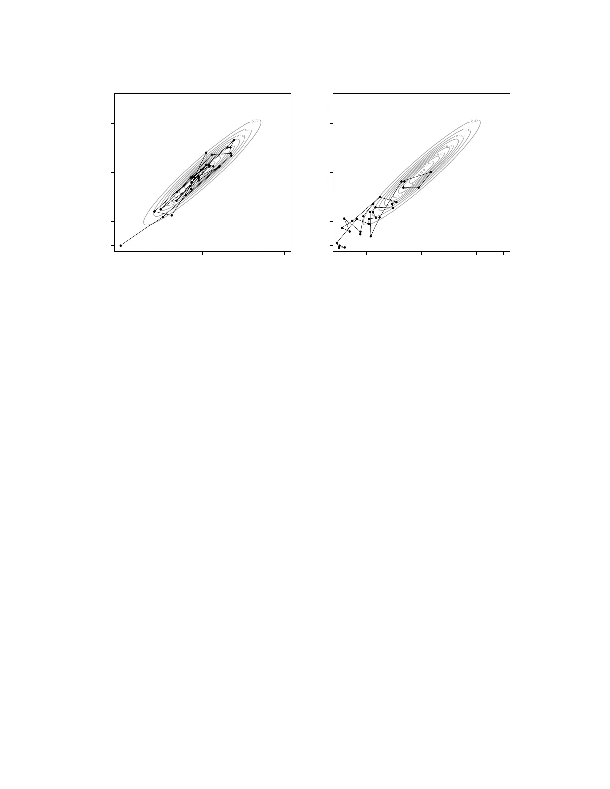
Loading high-quality paper...
Comments & Academic Discussion
Loading comments...
Leave a Comment