A Mechanistic Dynamic Emulator

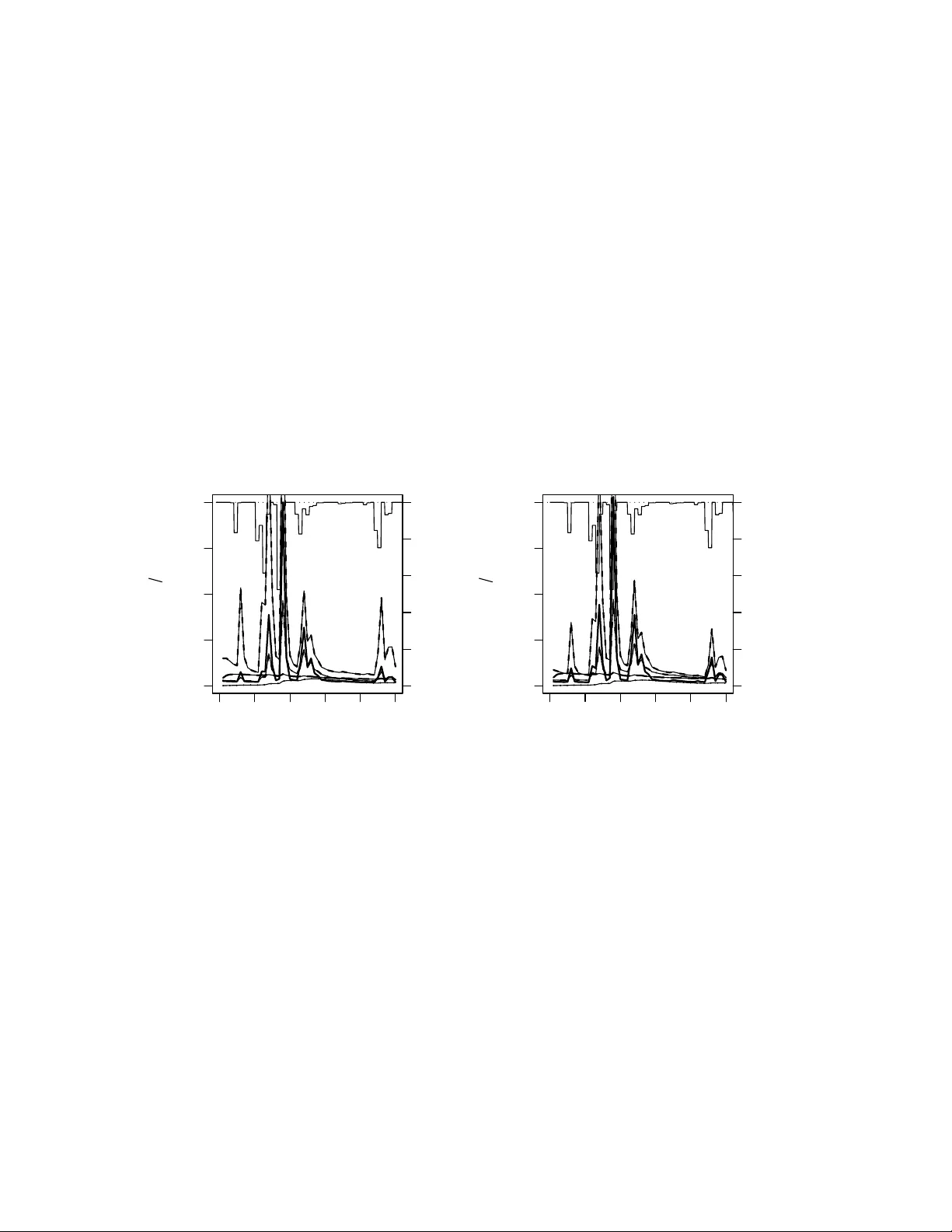
A Mec hanistic Dynamic Em ulator C. Alb ert ∗ Octob er 1, 2018 Abstract In applied sciences, w e often deal with deterministic sim ulation mo dels that are too slo w for sim ulation-in tensive tasks suc h as calibration or real-time con trol. In this pa- p er, an em ulator for a generic dynamic mo del, giv en by a system of ordinary non-linear differen tial equations, is developed. The non-linear differen tial equations are linearized and Gaussian white noise is added to accoun t for the non-linearities. The resulting linear sto c hastic system is conditioned on a set of solutions of the non-linear equations that ha ve b een calculated prior to the emulation. A path-integral approac h is used to derive the Gaussian distribution of the emulated solution. The solution reveals that most of the computational burden can b e shifted to the conditioning phase of the emulator and the complexit y of the actual emulation step only scales lik e O ( N n ) in m ultiplications of ma- trices of the dimension of the state space. Here, N is the n umber of time-points at which the solution is to b e emulated and n the num b er of solutions the emulator is conditioned on. The applicabilit y of the algorithm is demonstrated with the hydrological model logSPM. Keyw ords: dynamic emulator, path-integral 1 In tro duction In applied sciences, we often ha ve deterministic simulation mo dels at hand that are, although quite accurate, too slo w for many simulation-in tensiv e tasks such as calibration or real-time con trol. The purp ose of an emulator (e.g. [5]) is a fast in terp olation of the resp onse surface of the model. Therefore, the slow deterministic simulation model is simplified and noise is added to account for the errors due to simplification. The resulting fast sto chastic mo del is then conditioned with outputs from the sim ulation mo del that hav e b een produced off-line, that is, prior to the actual emulation. In this pap er, w e focus on dynamic mo dels, i.e., models describ ed by ODE’s whose outputs are giv en b y time-series. T reating time as an additional output comp onent or as an additional input [4] and applying a standard Gaussian emulator leads to an emulation time that gro ws quadratically with the num b er of time p oints, whic h is inefficien t if the num b er of time p oints is large. Emulators for the time-stepping [2], [3] hav e the disadv an tage that the whole state- space must b e emulated if one wan ts to retain the Marko v prop erty of the pro cess. Simplified mo dels in the form of sto c hastic linear models [8] or linear com binations of (wa velet) basis functions [1] hav e b een used as well. But none of the mentioned approac hes uses kno wledge ∗ Ea wag, aquatic researc h, 8600 D ¨ ub endorf, Switzerland. 1 ab out the dynamics of the sim ulation mo del, whic h we might retriev e, e.g., by linearizing its equations. Recen tly , Reichert et al. [9] developed a dynamic emulator whose underlying simplified model is a linear stochastic pro cess that captures the first order dynamics of the mo del. That is, their em ulator is to some exten t me chanism-b ase d and not merely statistical. F urthermore, they applied a Kalman filter in order for the complexity to grow only linearly with the num b er of time p oin ts. The inten tion b ehind this pap er is to further impro ve the computational efficiency of the em ulator presen ted in [9]. I start with a time-contin uous linear sto c hastic pro cess whose drift is assumed to b e given b y the linearization of the sim ulation mo del and whose noise is assumed to account for the non-linearities. This is the same as in [9], except that in [9] the noise is not in tegrated b etw een time steps. F or piece-wise constant input, I deriv e an analytic solution for the Gaussian distribution describing the emulated output. F or this purp ose, a path-integral approac h seems to b e adequate. The analytic solution reveals that most of the computational burden can be shifted to the conditioning phase of the em ulator so that w e are left with a computational complexity for the em ulation step that grows lik e O ( N n ) in m ultiplications of matrices of the dimension of the state space, m . Here, N is the num b er of time p oin ts and n the num b er of simulation outputs on which the sto c hastic mo del is conditioned. This is quite a substan tial impro vemen t of the algorithm presen ted in [9], whose emulation step needs O ( N ) m ultiplications of matrices of dimension nm as well as inv ersions of matrices of dimension m . Just like in [9], the algorithm is then tested with the hydrological mo del logSPM. 2 A Generic Dynamic Em ulator Consider a state sp ac e V of dimension m , whose elemen ts shall b e denoted b y ξ ξ ξ , and a deterministic simulation mo del , given by a system of ordinary differential equations ˙ ξ ξ ξ ( t ) = f ( ξ ξ ξ ( t ) , x ( t )) , (1) where x ∈ W denotes inputs and/or parameters and can be time-v arying. Subsequen tly , I refer to x as input and usually omit its time argument. The idea behind the em ulator is, firstly , to line arize eq. (1) and pac k all the non-linearities in to a noise term that is mo deled with a standard Wiener pro cess η η η ( t ) (i.e. Gaussian white noise). The co v ariance of the noise, C , is assumed to b e indep endent of the input. Thus, the linear sto chastic approximation to (1) is given by the system of linear sto chastic differential equations ˙ ξ ξ ξ ( t ) = A ( x ) ξ ξ ξ ( t ) + b ( x ) + C η η η ( t ) . (2) Secondly , n + 1 r eplic a of the system ar e c ouple d . Therefore, replace V b y V ⊗ R n +1 and W by W = W ⊗ R n +1 . Henceforth, v ectors without indices will denote elements of these extended spaces. The n + 1 replica are associated with n + 1 different inputs, x α . The first n inputs are those for whic h solutions of (1) are calculated that will b e used for the conditioning while the ( n + 1)th input is the one for whic h a solution is to b e em ulated. The replica are assumed to couple through the noise term only . Th us, A ( x ) and b ( x ) now denote the tensors A α β ( x ) = A ( x α ) δ α β , (3) b α ( x ) = b ( x α ) . (4) 2 The closer the inputs (measured with some metric ρ on W ) the stronger the associated replica are assumed to couple. Hence, set ˜ C ( x ) = C ⊗ R ( x ) , with R αβ ( x ) = exp( − ρ ( x α , x β ) / 2) . Th us, the emulator is describ ed b y the nm coupled linear sto chastic differential equations ˙ ξ ξ ξ ( t ) = A ( x ) ξ ξ ξ ( t ) + b ( x ) + ˜ C ( x ) η η η ( t ) . (5) Next, I derive the probability densit y of ξ ξ ξ ( t ) on the space of paths [ t 0 , t N ] − → V ⊗ R n +1 , with initial condition ξ ξ ξ ( t 0 ) = 0 . (6) It reads P [ ξ ξ ξ ( t )] ∝ exp  − 1 2 Z t N t 0  ˙ ξ ξ ξ ( t ) − A ( x ) ξ ξ ξ ( t ) − b ( x )  † ( ˜ C ˜ C T ) − 1 ( x )  ˙ ξ ξ ξ ( t ) − A ( x ) ξ ξ ξ ( t ) − b ( x )  dt  = exp  − 1 2 Z t N t 0  ξ ξ ξ ( t ) − D − 1 b ( x )  † ( D † ( ˜ C ˜ C T ) − 1 D )( x )  ξ ξ ξ ( t ) − D − 1 b ( x )  dt  , (7) where D = ∂ ∂ t − A ( x ) . (8) T o pro ceed, I need to determine the Gr e en ’s function of D . The most general solution of D ( t ) G ( t, t 0 ) = δ ( t − t 0 ) (9) is given by (see, e.g., [6] Chapter 3.3) G ( t, t 0 ) = ( ¯ Θ( t − t 0 ) + c ( t 0 )) P exp  Z t t 0 A ( x ( τ )) dτ  , (10) where ¯ Θ( t − t 0 ) is the regularized Heavyside function with ¯ Θ(0) = 1 / 2 and P denotes path- ordering of the exp onential. The function c ( t 0 ) is determined by the b oundary condition (6), whic h entails G ( t 0 , t ) = 0 , and translates into c ( t 0 ) ≡ 0 . Then, the adjoint Green’s function reads as G † ( t, t 0 ) = ¯ Θ( t 0 − t ) P exp  − Z t t 0 A T ( x ( τ )) dτ  . (11) No w, I calculate the c orr elation functions for tw o replica at tw o different time p oints, as expressed by the m × m matrices ˜ Σ αβ ij = h ξ ξ ξ α ( t i ) ⊗ ξ ξ ξ β ( t j ) i = Z − 1 Z exp  − 1 2 ξ ξ ξ † ( t ) D † ( ˜ C ˜ C T ) − 1 D ( x ) ξ ξ ξ ( t )  ξ ξ ξ α ( t i ) ⊗ ξ ξ ξ β ( t j ) D ξ ξ ξ , (12) 3 with Z = Z exp  − 1 2 ξ ξ ξ † ( t ) D † ( ˜ C ˜ C T ) − 1 D ( x ) ξ ξ ξ ( t )  D ξ ξ ξ . Using (10) and (11) one finds that, for t i ≥ t j , ˜ Σ αβ ij = Z t j t 0 P exp  Z t i t 0 A ( x α ( τ )) dτ  ( ˜ C ˜ C T ) αβ ( x ( t 0 )) P exp " − Z t 0 t j A T ( x β ( τ )) dτ # dt 0 . (13) F or t i < t j , one may use the symmetry relations ˜ Σ αβ ij = ( ˜ Σ β α j i ) T . (14) All finite dimensional mar ginals of (7) will b e Gaussians. I consider the finite-dimensional subspace of those comp onents of the first n replica that are sim ulated with (1) and those comp onen ts of the ( n + 1)th replica that shall b e em ulated, b oth at time points t 0 < t 1 < · · · < t N . Therefore, I introduce the op erator H ( x ) that is defined as ( H ( x )[ ξ ξ ξ ( t )]) α i = H ( x α ( t i )) ξ ξ ξ α ( t i ) , (15) where, on the r.h.s., H ( x α ( t i )) =: H α i denotes matrices of constant rank m 0 < m . The image of (15) is supp osed to b e determined by eq. ( H ( x )[ ξ ξ ξ ( t )]) α i = y α i . (16) In tegrating out all degrees of freedom that are not determined b y (16) yields the Gaussian distribution 1 Z − 1 Z P [ ξ ξ ξ ( t )] δ ( H [ ξ ξ ξ ( t )] − y ) D ξ ξ ξ ∝ Z exp  − 1 2 Z ξ ξ ξ † ( t ) D † ( ˜ C ˜ C T ) − 1 Dξ ξ ξ ( t ) dt  δ ( H [ ξ ξ ξ ( t )] − ( y − H D − 1 b )) D ξ ξ ξ ∝ exp  − 1 2 ( y − H D − 1 b ) † Σ − 1 ( y − H D − 1 b )  , (17) with cov ariance matrix Σ = H D − 1 ( ˜ C ˜ C T )( D † ) − 1 H † , (18) and mean z = H D − 1 b . (19) The cov ariance matrix is a square matrix of dimension ( n + 1) N m 0 , whose m 0 × m 0 blo c ks are giv en by the equations Σ αβ ij = H α i ˜ Σ αβ ij ( H β j ) T , (20) with ˜ Σ as defined by (13) and (14). Finally , I determine the Gaussian distribution for the ( n + 1) th r eplic a (the online system) , conditioned on the sim ulations y a i , for i = 1 , . . . , N and a = 1 , . . . , n . Therefore, I split the ( n + 1)th replica off, writing Σ as the blo c k matrix Σ =   Σ n +1 ,n +1 Σ n +1 ,. Σ .,n +1 Σ 0   . (21) 1 T o keep the notation simple, w e will omit the dependence of H , D , ˜ C , and b on x subsequen tly . 4 Mean and cov ariance matrix of the online system are given b y equations ¯ y = z n +1 + Σ n +1 ,a (Σ 0 ) − 1 ab ( y b − z b ) , (22) ¯ Σ = Σ n +1 ,n +1 − Σ n +1 ,a (Σ 0 ) − 1 ab Σ b,n +1 , (23) where a and b run from 1 to n only . Note that eq. (22) is translational inv arian t. Thus, one ma y replace condition (6) by ξ ξ ξ (0) = ξ ξ ξ 0 . (24) In the remainder of this c hapter, a recursive pro cedure of calculating (22) and (23) is dev elop ed. Due to path-ordering eqs. (13) and (20) can b e written as Σ αβ ij = H α i  j − 1 X k =0 h α i − 1 . . . h α k +1 g αβ k h † β k +1 . . . h † β j − 1  ( H β j ) T , (25) with g αβ k = Z t k +1 t k P exp  Z t k +1 t 0 A ( x α ( τ )) dτ  ( ˜ C ˜ C T ) αβ ( t 0 ) P exp " − Z t 0 t k +1 A T ( x β ( τ )) dτ # , (26) h α l = P exp  Z t l +1 t l A ( x α ( τ )) dτ  , (27) h † α l = P exp " − Z t l t l +1 A T ( x α ( τ )) dτ # . (28) The b oundary conditions (6) or (24) imply the initial v ariances Σ αβ 00 = 0 . (29) In the c onditioning step of the algorithm one calculates (Σ 0 ) − 1 and z a , for a = 1 , . . . , n . F or the former, use (14), (20) and (29) and, for j ≤ i , the recursion relations Σ αβ i +1 ,j = h α i Σ αβ ij (30) Σ αβ ii = Σ αβ i,i − 1 h † β i − 1 + g αβ i − 1 . (31) F or the latter, set z α i = H α i ˜ z α i , and use the recursion relations ˜ z α i +1 = h α i ˜ z α i + k α i , ˜ z α 0 = 0 , (32) with k α i = Z t i +1 t i P exp  Z t i +1 t 0 A ( x α ( τ )) dτ  b α ( t 0 ) dt 0 . (33) Once (Σ 0 ) − 1 and all the z a are calculated, pre-calculate, for the em ulation step, the cov ectors z 0 ia := T a ij ( H a j ) T ((Σ 0 ) − 1 ) j k ab ( y b k − z b k ) , (34) 5 where, on the r.h.s., the i ’s and the a ’s are not summed ov er and with T a ij :=    h † a i +1 . . . h † a j − 1 , j ≥ i + 2 , 1 , j = i + 1 , 0 , else . (35) In the actual emulation step calculate (22) setting ¯ y i = H n +1 i ˜ y i , (36) and using the recursion relation ˜ y i +1 = h n +1 i ˜ y i + k n +1 i + g n +1 ,a i z 0 ia , (37) with z 0 ia as defined in (34). In order to get the start v alue, ˜ y 1 , one needs to calculate Σ n +1 ,a 1 j using (14), (29) and the recursion relations (30) and (31). The computational complexity of the emulation ste p is of the order O ( N n ) in matrix multiplications of dimension m . If one is in terested in the v ariances, i.e., the diagonal elemen ts of ¯ Σ, one may derive a similar recursion form ula for them. Since path-ordered exp onentials can, in general, not b e calculated analytically , I consider the sp ecial case of pie c e-wise c onstant input x α ( t ) = x α i , t i ≤ t ≤ t i +1 . Then, (26), (27) and (33) reduce to g αβ k = ( R αβ k ) 2 Z t k +1 t k e ( t k +1 − t 0 ) A ( x α k ) C C T e ( t k +1 − t 0 )( A ( x β k )) T dt 0 , (38) h α l = e ( t l +1 − t l ) A ( x α l ) , (39) k α i = Z t i +1 t i e ( t i +1 − t 0 ) A ( x α i ) b α i dt 0 . (40) If A ( x ) is diagonalizable , functions (38) through (40) can b e obtained analytically . F or A ( x α k ) = M α k diag o [ λ α o ] ( M α k ) − 1 , one gets g αβ k = ( R αβ k ) 2 M α k B αβ k ( M β k ) T , (41) with ( B αβ k ) p q = exp(( t k +1 − t k )( λ α k,p + λ β k,q )) − 1 λ α k,p + λ β k,q (( M α k ) − 1 C C T (( M β k ) − 1 ) T ) p q , (42) and h α l = M α l diag o  exp(( t l +1 − t l ) λ α l,o )  ( M α l ) − 1 , (43) and k α i = M α i diag o " exp(( t i +1 − t i ) λ α i,o ) − 1 λ α i,o # ( M α i ) − 1 b α i . (44) 6 If x is time-independent (e.g. parameters of the mo del) and A ( x ) diagonalizable, (20) can b e calculated explicitly . If A ( x α ) = M α diag o [ λ α o ] ( M α ) − 1 , one derives from (20) that, for t i > t j , ˜ Σ αβ ij = ( R αβ ) 2 M α B αβ ij ( M β ) T , where ( B αβ ij ) p q = (( M α ) − 1 C C T (( M β ) T ) − 1 ) p q Z t j t 0 exp[ t i λ α p + t j λ β q − t 0 ( λ α p + λ β q )] dt 0 = (( M α ) − 1 C C T (( M β ) T ) − 1 ) p q exp  ( t i − t 0 ) λ α p + ( t j − t 0 ) λ β q  − exp  ( t i − t j ) λ α p  λ α p + λ β q . (45) 3 Hydrological Application In this section, the algorithm dev elop ed in the last section is tested with a simple h ydrological mo del called logSPM [7]. The state vector of this mo del is three-dimensional, ξ ξ ξ = ( h s , h g w , h r ) T , (46) and describes the amoun t of w ater stored in the soil, the ground-water and the river. The dynamics is describ ed by the system of ordinary differential equations ˙ h s = q rain − q runof f − q et − q lat − q g w , (47) ˙ h g w = q g w − q bf − q dp , (48) ˙ h r = q runof f + q lat + q bf − q r , (49) and visualized in Fig. 1. The fluxes are giv en by the equations q rain = i rain ( t ) , q runof f = f sat i rain ( t ) , (50) q et = f et i pet ( t ) , q lat = f sat q lat,max , (51) q g w = f sat q g w,max , q bf = k bf h g w , (52) q dp = k dp h g w , q r = k r h r , (53) with the fraction of saturated area, f sat , given by equation f sat = 1 1 + s F e − k s h s − 1 1 + s F , (54) and the fraction of actual ev ap otranspiration, f et , given by equation f et = 1 − e − k et h s . (55) The output of the mo del is the river flow, Q r , given as Q r = A W q r , 7 where A W is the area of watershed. The linearization of the mo del equations reads: ˙ ξ ξ ξ ( t ) = A ( x ) ξ ξ ξ ( t ) + b ( x ) , (56) with A ( x ) =   λ 1 ( t ) 0 0 a λ 2 0 c ( t ) b λ 3   , b ( x ) =   i rain ( t ) 0 0   , (57) and x ( t ) = ( λ 1 ( t ) , λ 2 , λ 3 , a, b, c ( t ) , i rain ( t )) T , with a = a sat q g w,max , b = k bf , c ( t ) = a sat ( i rain ( t ) + q lat,max ) , (58) and λ 1 ( t ) = − a sat ( i rain ( t ) + q lat,max + q g w,max ) − a et i pet ( t ) , λ 2 = − k bf − k dp , λ 3 = − k r . (59) The functions (54) and (55) w ere appro ximated by linear functions that intersect the nonlinear functions at h s, 1 and h s, 2 , resp ectively . See Fig. 2. Therefore, a sat = 1 h s, 1  1 1 + s F e − k s g h s, 1 − 1 1 + s F  , and a et = 1 h s, 2  1 − e − k et h s, 2  . Only the inputs i rain and i pet are time-dep endent, and, therefore, c , b and λ 1 . The observ ation matrices read as H α =   0 0 0 0 0 0 0 0 − A W λ α 3   . (60) I choose the Euclidean metric on the space of parameters R 8 3 θ θ θ = ( k s , s F , k et , q lat,max , q g w m ax , k bf , k dp , k r ) T , where each comp onen t is normalized with a reasonable range. The noise C w as c hosen to b e diagonal and the diagonal entries to b e a certain fraction of the initial condition ξ ξ ξ 0 . Ob viously , A ( x ) is diagonalizable: M − 1 ( t ) A ( x ) M ( t ) = diag o [ λ o ] , (61) with M ( t ) =    1 0 0 a λ 1 − λ 2 1 0 c ( λ 1 − λ 2 )+ ab ( λ 1 − λ 2 )( λ 1 − λ 3 ) b λ 2 − λ 3 1    , (62) and the matrices (41), (43) and (44) can b e calculated analytically . Plot 3 compares solutions of the full mo del with emulated solutions for 5 randomly chosen sets of parameters (that were not used for the conditioning of the em ulator). The results are v ery similar to those obtained in [9]. F or an extended statistical analysis of the p erformance of the emulator, I refer to [9]. 8 4 Conclusions I ha ve presented an explicit solution for the em ulation of the time-series of a dynamic mo del. In general, the path-ordered exp onen tials the solution is expressed with cannot b e calculated analytically . Therefore, I resort to piece-wise constan t inputs. Then, the em ulator presented in this pap er is the same as the one presen ted in [9], except that I integrate the noise betw een time steps. F or piece-wise constant input, this can b e done at negligible additional cost and p oten tially increases the quality of the em ulation. The exact solution presented in eqs. (22) and (23) allows for an efficien t n umerical imple- men tation that is of the order O ( nN ) in matrix m ultiplications of dimension m . The Kalman filtering and smo othing algorithm used in [9] needs O ( N ) matrix multiplications of dimension nm and matrix inv ersions of dimension m . The disadv antage of my metho d, how ev er, as compared to the one presen ted in [9] is the fact that a huge matrix of dimension N nm 0 needs to b e in verted for the conditioning, which migh t b e challenging b oth for the memory and the CPU. Ac kno wledgments: I’m indebted to Peter Reichert for man y fruitful discussions ab out emulators as well as many lines of R Co de for the presentation of the results. References [1] M. J. Ba yarri, J. O. Berger, J. Cafeo, G. Garcia-Donato, F. Liu, J. P alomo, R. J. P arthasarathy , R. P aulo, J. Sacks, and D. W alsh. Computer mo del v alidation with func- tional output. Ann. Stat. , 35(5):1874–1906, 2007. [2] S. Bhattachary a. A sim ulation approach to bay esian em ulation of complex dynamic com- puter mo dels. Bayesian Analysis , 2:783–816, 2007. [3] S. Conti, J. P . Gosling, J. Oakley , and A. O’Hagan. Gaussian pro cess emulation of dynamic computer co des. Biometrika , 96(3):663–676, 2009. [4] S. Conti and A. O’Hagan. Ba yesian emulation of complex multi-output and dynamic computer mo dels. J. Stat. Planning and Infer enc e , 140:640–651, 2010. [5] M. C. Kennedy and A. O’Hagan. Bay esian calibration of computer mo dels. J. R oy. Stat. So c. B , 63(3):425–464, 2001. [6] H. Kleinert. Path inte gr als in quantum me chanics, statistics, p olymer physics, and finan- cial markets (5th e d.) . W orld Scientific Publishing, Singap ore, 2009. [7] G. Kuczera, D. Kav etski, S. F ranks, and M. Th y er. T ow ards a Ba y esian total error analysis of conceptual rainfall-runoff models: Characterising mo del error using storm-dependent parameters. J. Hydr olo gy , 331(1-2):161–177, 2006. [8] F. Liu and M. W est. A dynamic mo delling strategy for Bay esian computer mo del emula- tion. J. Bayesian Anal. , 4(2):393–412, 2009. 9 [9] P . Reichert, G. White, M. J. Bay arri, and E. B. Pitman. Mechanism-based em ulation of dynamic sim ulation mo dels: Concept and application in hydrology . J. Comp. Stat. Dat. A nal. , 55:1638–1655, 2011. 10 soil ground water river q et q rain q runoff q lat q gw q bf q r q dp Figure 1: Visualization of the fluxes in the mo del logSPM. T ak en from J. Comp. Stat. and Data Analysis. 0 100 200 300 400 500 0.0 0.2 0.4 0.6 0.8 1.0 h s [mm] f sat [−] k.s=0.02/mm, s.F=300 k.s=0.01/mm, s.F=300 k.s=0.02/mm, s.F=100 0 100 200 300 400 500 0.0 0.2 0.4 0.6 0.8 1.0 h s [mm] f et [−] k.et=0.01/mm k.et=0.02/mm k.et=0.005/mm Figure 2: Shap e of the nonlinear functions used for describing some fluxes in the hydrological mo del. F raction of saturated are, left, and fraction of actual ev ap otranspiration, righ t. The b old parts of the curv es represent the range of v alues co vered in the base simulation. The straigh t lines represent linearizations that in tersect the nonlinear function at giv en v alues of h s . T aken from J. Comp. Stat. and Data Analysis. 11 0 10 20 30 40 50 0 100 200 300 400 model t [da ys] Q [ m 3 s ] 100 80 60 40 20 0 i rain [mm/d] 0 10 20 30 40 50 0 100 200 300 400 emulator t [da ys] Q [ m 3 s ] 100 80 60 40 20 0 i rain [mm/d] d = 11.4 Figure 3: Comparison of simulations of the full mo del (left) with em ulations (right) for 5 randomly chosen sets of parameters. The dominant mo del input, rain intensit y , is plotted from the top (right scale). The emulator w as conditioned with 50 sets of parameters. The d -v alue is the square ro ot of the mean sum of squares. 12