On the Robustness of Most Probable Explanations
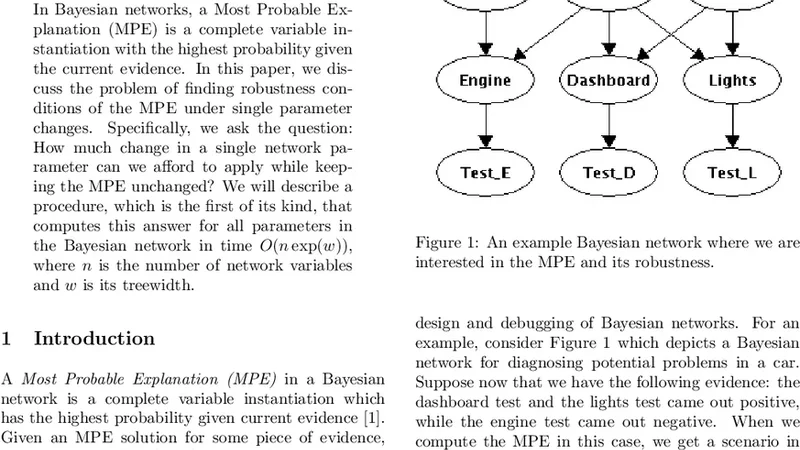
In Bayesian networks, a Most Probable Explanation (MPE) is a complete variable instantiation with a highest probability given the current evidence. In this paper, we discuss the problem of finding robustness conditions of the MPE under single parameter changes. Specifically, we ask the question: How much change in a single network parameter can we afford to apply while keeping the MPE unchanged? We will describe a procedure, which is the first of its kind, that computes this answer for each parameter in the Bayesian network variable in time O(n exp(w)), where n is the number of network variables and w is its treewidth.
💡 Research Summary
The paper tackles a previously under‑explored aspect of inference in Bayesian networks: the robustness of a Most Probable Explanation (MPE) with respect to changes in a single network parameter. An MPE is the complete assignment of all variables that maximizes the posterior probability given observed evidence. While many works have focused on efficiently computing the MPE or on measuring the margin between the MPE and the second‑best explanation, none have provided a systematic method for quantifying exactly how much a single conditional‑probability table (CPT) entry can be perturbed before the MPE switches to a different assignment.
The authors formalize this question as “what is the maximal allowable deviation of a single parameter such that the current MPE remains optimal?” They then derive a procedure that answers the question for every parameter in the network in time O(n·exp(w)), where n is the number of variables and w is the treewidth of the underlying graph. The key technical insight is that the log‑probability difference Δ between the current MPE and the best competing explanation (the second‑best explanation, SBE) is a linear function of any individual CPT entry. By representing Δ(θ_i) = a_i·θ_i + b_i, the condition Δ > 0 translates into a simple linear inequality that defines an interval of admissible values for θ_i.
To compute the coefficients a_i and b_i efficiently, the algorithm first constructs a tree decomposition of the Bayesian network, yielding a set of clusters (bags) whose size is bounded by w + 1. Using standard message‑passing (belief propagation) on this junction tree, the algorithm evaluates the contribution of each cluster to the log‑probability of the MPE and of the SBE. Because each cluster contains only O(exp(w)) states, the per‑cluster work is exponential only in the treewidth, not in the total number of variables. By aggregating the contributions across all clusters, the algorithm obtains the exact linear relationship for each parameter.
The procedure consists of the following steps:
- Build a tree decomposition and run a forward‑backward pass to compute the usual belief‑propagation messages.
- Identify the current MPE and the SBE using any exact MPE algorithm (e.g., variable elimination or bucket elimination).
- For each parameter θ_i, record how the log‑probability of the MPE and the SBE would change if θ_i were perturbed; this yields the slope a_i. The intercept b_i is the current log‑probability gap.
- Solve the inequality a_i·θ_i + b_i > 0 for θ_i ∈