A Scalable Bootstrap for Massive Data

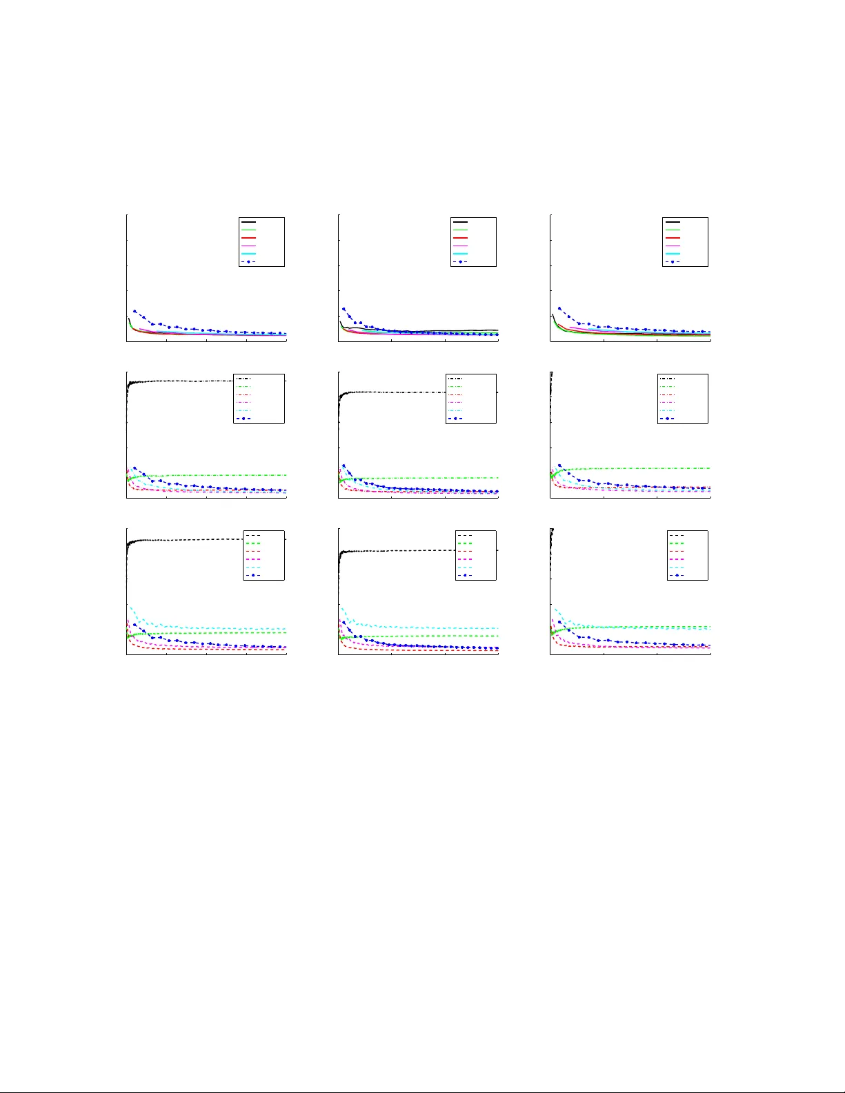
A Scalable Bo otstrap for Massiv e Data Ariel Kleiner Departmen t of Electrical Engineering and Computer Science Univ ersity of California, Berk eley akleiner@eecs.berkeley.edu Ameet T alw alk ar Departmen t of Electrical Engineering and Computer Science Univ ersity of California, Berk eley ameet@eecs.berkeley.edu Purnamrita Sark ar Departmen t of Electrical Engineering and Computer Science Univ ersity of California, Berk eley psarkar@eecs.berkeley.edu Mic hael I. Jordan Departmen t of Statistics and Departmen t of Electrical Engineering and Computer Science Univ ersity of California, Berk eley jordan@eecs.berkeley.edu No vem b er 27, 2024 Abstract The bo otstrap pro vides a simple and pow erful means of assessing the qualit y of esti- mators. Ho w ever, in settings inv olving large datasets—which are increasingly prev alen t— the computation of b o otstrap-based quan tities can b e prohibitiv ely demanding com- putationally . While v ariants suc h as subsampling and the m out of n b o otstrap can b e used in principle to reduce the cost of b o otstrap computations, w e ﬁnd that these meth- o ds are generally not robust to speciﬁcation of hyperparameters (such as the num b er of subsampled data p oints), and they often require use of more prior information (such as rates of conv ergence of estimators) than the b o otstrap. As an alternative, we intro- duce the Bag of Little Bo otstraps (BLB), a new pro cedure which incorp orates features of b oth the b o otstrap and subsampling to yield a robust, computationally eﬃcien t 1 means of assessing the quality of estimators. BLB is well suited to mo dern parallel and distributed computing architectures and furthermore retains the generic applicabilit y and statistical eﬃciency of the b o otstrap. W e demonstrate BLB’s fav orable statistical p erformance via a theoretical analysis elucidating the pro cedure’s prop erties, as w ell as a sim ulation study comparing BLB to the b o otstrap, the m out of n b o ots trap, and subsampling. In addition, we present results from a large-scale distributed implemen- tation of BLB demonstrating its computational sup eriority on massive data, a metho d for adaptiv ely selecting BLB’s h yp erparameters, an empirical study applying BLB to sev eral real datasets, and an extension of BLB to time series data. 1 In tro duction The dev elopmen t of the b o otstrap and related resampling-based methods in the 1960s and 1970s heralded an era in statistics in whic h inference and computation became increasingly in tertwined (Efron, 1979; Diaconis and Efron, 1983). By exploiting the basic capabilities of the classical von Neumann computer to simulate and iterate, the bo otstrap made it p ossible to use computers not only to compute estimates but also to assess the qualit y of estimators, yielding results that are quite generally consistent (Bic k el and F reedman, 1981; Gin´ e and Zinn, 1990; v an der V aart and W ellner, 1996) and often more accurate than those based up on asymptotic appro ximation (Hall, 1992). Moreo ver, the b o otstrap aligned statistics to computing tec hnology , suc h that adv ances in sp eed and storage capacity of computers could immediately allo w statistical metho ds to scale to larger datasets. Tw o recen t trends are w orthy of atten tion in this regard. First, the growth in size of datasets is accelerating, with “massive” datasets b ecoming increasingly prev alent. Sec- ond, computational resources are shifting tow ard parallel and distributed architectures, with m ulticore and cloud computing platforms providing access to hundreds or thousands of pro- cessors. The second trend is seen as a mitigating factor with resp ect to the ﬁrst, in that parallel and distributed arc hitectures presen t new capabilities for storage and manipulation of data. Ho w ever, from an inferential point of view, it is not y et clear ho w statistical method- ology will transp ort to a world in volving massiv e data on parallel and distributed computing platforms. While massive data bring many statistical issues to the fore, including issues in ex- ploratory data analysis and data visualization, there remains the core inferen tial need to assess the quality of estimators. Indeed, the uncertain t y and biases in estimates based on large data can remain quite signiﬁcan t, as large datasets are often high dimensional, are frequen tly used to ﬁt complex mo dels with large n um b ers of parameters, and can hav e many p oten tial sources of bias. F urthermore, ev en if suﬃcient data are a v ailable to allo w highly accurate estimation, the ability to eﬃcien tly assess estimator quality remains essen tial to allo w eﬃcien t use of a v ailable resources by pro cessing only as m uc h data as is necessary to ac hieve a desired accuracy or conﬁdence. The bo otstrap brings to b ear v arious desirable features in the massiv e data setting, notably its relativ ely automatic nature and its applicabilit y to a wide v ariety of inferen tial 2 problems. It can b e used to assess bias, to quantify the uncertaint y in an estimate (e.g., via a standard error or a conﬁdence in terv al), or to assess risk. How ev er, these virtues are realized at the expense of a substantial computational burden. Bo otstrap-based quan tities t ypically must be computed via a form of Mon te Carlo appro ximation in whic h the estimator in question is rep eatedly applied to resamples of the en tire original observed dataset. Because these resamples hav e size on the order of that of the original data, with appro x- imately 63% of data points appearing at least once in eac h resample, the usefulness of the b o otstrap is sev erely blun ted b y the large datasets increasingly encountered in practice. In the massive data setting, computation of even a single p oint estimate on the full dataset can be quite computationally demanding, and so repeated computation of an estimator on comparably sized resamples can b e prohibitiv ely costly . T o mitigate this problem, one migh t naturally attempt to exploit the mo dern trend tow ard parallel and distributed computing. Indeed, at ﬁrst glance, the b o otstrap w ould seem ideally suited to straigh tforwardly lev er- aging parallel and distributed computing arc hitectures: one migh t imagine using diﬀerent pro cessors or compute no des to pro cess diﬀeren t b o otstrap resamples indep endently in par- allel. How ev er, the large size of b o otstrap resamples in the massive data setting renders this approac h problematic, as the cost of transferring data to indep endent processors or compute no des can b e ov erly high, as is the cost of op erating on even a single resample using an indep enden t set of computing resources. While the literature do es con tain some discussion of tec hniques for impro ving the com- putational eﬃciency of the bo otstrap, that w ork is largely dev oted to reducing the num b er of resamples required (Efron, 1988; Efron and Tibshirani, 1993). These tec hniques in general in tro duce signiﬁcant additional complexity of implementation and do not eliminate the crip- pling need for rep eated computation of the estimator on resamples ha ving size comparable to that of the original dataset. Another landmark in the developmen t of simulation-based inference is subsampling (Poli- tis et al., 1999) and the closely related m out of n b o otstrap (Bic kel et al., 1997). These metho ds (which were in tro duced to achiev e statistical consistency in edge cases in whic h the b o otstrap fails) initially appear to remedy the b o otstrap’s k ey computational shortcoming, as they only require rep eated computation of the estimator under consideration on resam- ples (or subsamples) that can b e signiﬁcantly smaller than the original dataset. Ho w ev er, these pro cedures also ha ve dra wbacks. As we sho w in our sim ulation study , their success is sensitiv e to the c hoice of resample (or subsample) size (i.e., m in the m out of n b o otstrap). Additionally , b ecause the v ariabilit y of an estimator on a subsample diﬀers from its v ari- abilit y on the full dataset, these pro cedures m ust p erform a rescaling of their output, and this rescaling requires knowledge and explicit use of the con vergence rate of the estimator in question; these metho ds are thus less automatic and easily deploy able than the b o ot- strap. While sc hemes ha ve b een proposed for data-driv en selection of an optimal resample size (Bic k el and Sak ov, 2008), they require signiﬁcan tly greater computation whic h w ould eliminate an y computational gains. Also, there has been w ork on the m out of n b o otstrap that has sough t to reduce computational costs using tw o diﬀerent v alues of m in conjunc- tion with extrap olation (Bic kel and Y ahav, 1988; Bick el and Sak o v, 2002). How ev er, these 3 approac hes explicitly utilize series expansions of the estimator’s sampling distribution and hence are less automatically usable; they also require execution of the m out of n b o otstrap for m ultiple v alues of m . Motiv ated b y the need for an automatic, accurate means of assessing estimator quality that is scalable to large datasets, w e introduce a new pro cedure, the Bag of Little Bootstraps (BLB), whic h functions b y com bining the results of b o otstrapping multiple small subsets of a larger original dataset. Instead of applying an estimator directly to eac h small subset, as in the m out of n b o otstrap and subsampling, the Bag of Little Bo otstraps (BLB) applies the b o otstrap to each small subset, where in the resampling pro cess of eac h individual b o ot- strap run, w eighted samples are formed suc h that the eﬀect is that of sampling the small subset n times with replacement, but the computational cost is that asso ciated with the size of the small subset. This has the eﬀect that, despite op erating only on subsets of the original dataset, BLB does not require analytical rescaling of its output. Ov erall, BLB has a signiﬁcan tly more fa vorable computational proﬁle than the bo otstrap, as it only requires rep eated computation of the estimator under consideration on quantities of data that can b e m uch smaller than the original dataset. As a result, BLB is w ell suited to implemen tation on mo dern distributed and parallel computing arc hitectures which are often used to pro cess large datasets. Also, our pro cedure main tains the b o otstrap’s generic applicability , fav or- able statistical properties (i.e., consistency and higher-order correctness), and simplicit y of implemen tation. Finally , as w e sho w in experiments, BLB is consisten tly more robust than alternativ es such as the m out of n b o otstrap and subsampling. The remainder of our presentation is organized as follows. In Section 2, we formalize our statistical setting and notation, present BLB in detail, and discuss the procedure’s compu- tational characteristics. Subsequently , in Section 3, we elucidate BLB’s statistical prop erties via a theoretical analysis (Section 3.1) showing that BLB shares the bo otstrap’s consistency and higher-order correctness, as well as a sim ulation study (Section 3.2) which compares BLB to the b o otstrap, the m out of n b o otstrap, and subsampling. Section 4 discusses a large-scale implementation of BLB on a distributed computing system and presents results illustrating the pro cedure’s sup erior computational p erformance in the massive data setting. W e present a method for adaptively selecting BLB’s h yp erparameters in Section 5. Finally , w e apply BLB (as w ell as the b o otstrap and the m out of n b o otstrap, for comparison) to sev eral real datasets in Section 6, w e presen t an extension of BLB to time series data in Section 7, and w e conclude in Section 8. 2 Bag of Little Bo otstraps (BLB) 2.1 Setting and Notation W e assume that we observe a sample X 1 , . . . , X n ∈ X dra wn i.i.d. from some (unkno wn) underlying distribution P ∈ P ; w e denote by P n = n − 1 P n i =1 δ X i the corresp onding empirical distribution. Based only on this observ ed data, we compute an estimate ˆ θ n ∈ Θ of some (unkno wn) p opulation v alue θ ∈ Θ asso ciated with P . F or example, ˆ θ n migh t estimate a 4 measure of correlation, the parameters of a regressor, or the prediction accuracy of a trained classiﬁcation mo del. When w e wish to explicitly indicate the data used to compute an estimate, we shall write ˆ θ ( P n ). Noting that ˆ θ n is a random quantit y b ecause it is based on n random observ ations, we deﬁne Q n ( P ) ∈ Q as the true underlying distribution of ˆ θ n , whic h is determined b y b oth P and the form of the estimator. Our end goal is the computation of an estimator qualit y assessmen t ξ ( Q n ( P ) , P ) : Q × P → Ξ, for Ξ a v ector space; to ligh ten notation, w e shall interc hangeably write ξ ( Q n ( P )) in place of ξ ( Q n ( P ) , P ). F or instance, ξ migh t compute a quantile, a conﬁdence region, a standard error, or a bias. In practice, w e do not hav e direct kno wledge of P or Q n ( P ), and so we must estimate ξ ( Q n ( P )) itself based only on the observ ed data and knowledge of the form of the estimator under consideration. Note that w e allo w ξ to dep end directly on P in addition to Q n ( P ) b ecause ξ might op erate on the distribution of a centered and normalized v ersion of ˆ θ n . F or example, if ξ computes a conﬁdence region, it might manipulate the distribution of the statistic √ n ( ˆ θ n − θ ), whic h is determined b y b oth Q n ( P ) and θ ; because θ cannot in general b e obtained directly from Q n ( P ), a direct dep endence on P is required in this case. Nonetheless, given kno wledge of Q n ( P ), any direct dep endence of ξ on P generally has a simple form, often only in v olving the parameter θ . Additionally , rather than restricting Q n ( P ) to b e the distribution of ˆ θ n , we could instead allo w it to be the distribution of a more general statistic, suc h as ( ˆ θ n , ˆ σ n ), where ˆ σ n is an estimate of the standard deviation of ˆ θ n (e.g., this w ould apply when constructing conﬁdence in terv als based on the distribution of the studen tized statistic ( ˆ θ n − θ ) / ˆ σ n ). Our subsequen t dev elopment generalizes straigh tforwardly to this setting, but to simplify the exp osition, w e will largely assume that Q n ( P ) is the distribution of ˆ θ n . Under our notation, the b o otstrap simply computes the data-driv en plugin approximation ξ ( Q n ( P )) ≈ ξ ( Q n ( P n )). Although ξ ( Q n ( P n )) cannot b e computed exactly in most cases, it is generally amenable to straigh tforward Monte Carlo approximation via the following algorithm (Efron and Tibshirani, 1993): rep eatedly resample n points i.i.d. from P n , compute the estimate on eac h resample, form the empirical distribution Q ∗ n of the computed estimates, and appro ximate ξ ( Q n ( P )) ≈ ξ ( Q ∗ n ). Similarly , using our notation, the m out of n bo otstrap (and subsampling) functions as follo ws, for m < n (Bic k el et al., 1997; Politis et al., 1999): rep eatedly resample m points i.i.d. from P n (subsample m p oints without replacemen t from X 1 , . . . , X n ), compute the estimate on eac h resample (subsample), form the empirical distribution Q ∗ m of the computed estimates, appro ximate ξ ( Q m ( P )) ≈ ξ ( Q ∗ m ), and apply an analytical correction to in turn approximate ξ ( Q n ( P )). This ﬁnal analytical correction uses prior knowledge of the con vergence rate of ˆ θ n as n increases and is necessary b ecause each v alue of the estimate is computed based on only m rather than n p oin ts. W e use 1 d to denote the d -dimensional vector of ones, and w e let I d denote the d × d iden tity matrix. 2.2 Bag of Little Bo otstraps The Bag of Little Bo otstraps (BLB) functions by av eraging the results of b o otstrapping m ultiple small subsets of X 1 , . . . , X n . More formally , given a subset size b < n , BLB samples 5 s subsets of size b from the original n data points, uniformly at random (one can also imp ose the constraint that the subsets be disjoin t). Let I 1 , . . . , I s ⊂ { 1 , . . . , n } b e the corresp onding index multisets (note that |I j | = b, ∀ j ), and let P ( j ) n,b = b − 1 P i ∈I j δ X i b e the empirical distribution corresp onding to subset j . BLB’s estimate of ξ ( Q n ( P )) is then given b y s − 1 s X j =1 ξ ( Q n ( P ( j ) n,b )) . (1) Although the terms ξ ( Q n ( P ( j ) n,b )) in (1) cannot be computed analytically in general, they can b e computed n umerically via straigh tforward Mon te Carlo appro ximation in the manner of the b o otstrap: for eac h term j , rep eatedly resample n p oin ts i.i.d. from P ( j ) n,b , compute the estimate on each resample, form the empirical distribution Q ∗ n,j of the computed estimates, and appro ximate ξ ( Q n ( P ( j ) n,b )) ≈ ξ ( Q ∗ n,j ). No w, to realize the substan tial computational b eneﬁts aﬀorded by BLB, we utilize the follo wing crucial fact: eac h BLB resample, despite having nominal size n , con tains at most b distinct data p oints. In particular, to generate eac h resample, it suﬃces to dra w a v ector of counts from an n -trial uniform multinomial distribution ov er b ob jects. W e can then represen t eac h resample by simply main taining the at most b distinct p oin ts presen t within it, accompanied b y corresp onding sampled coun ts (i.e., each resample requires only storage space in O ( b )). In turn, if the estimator can work directly with this weigh ted data repre- sen tation, then the computational requirements of the estimator—with resp ect to b oth time and storage space—scale only in b , rather than n . F ortunately , this prop erty do es indeed hold for man y if not most commonly used estimators, such as general M-estimators. The resulting BLB algorithm, including Mon te Carlo resampling, is shown in Algorithm 1. Th us, BLB only requires rep eated computation on small subsets of the original dataset and a v oids the b o otstrap’s problematic need for rep eated computation of the estimate on resamples having size comparable to that of the original dataset. A simple and standard calculation (Efron and Tibshirani, 1993) shows that eac h b o otstrap resample contains ap- pro ximately 0 . 632 n distinct p oints, which is large if n is large. In contrast, as discussed ab o v e, each BLB resample con tains at most b distinct p oints, and b can b e chosen to b e m uch smaller than n or 0 . 632 n . F or example, we migh t take b = n γ where γ ∈ [0 . 5 , 1]. More concretely , if n = 1 , 000 , 000, then each b o otstrap resample w ould con tain appro ximately 632 , 000 distinct p oints, whereas with b = n 0 . 6 eac h BLB subsample and resample would con tain at most 3 , 981 distinct p oin ts. If eac h data p oin t o ccupies 1 MB of storage space, then the original dataset w ould o ccupy 1 TB, a b o otstrap resample w ould o ccupy approx- imately 632 GB, and each BLB subsample or resample w ould o ccupy at most 4 GB. As a result, the cost of computing the estimate on eac h BLB resample is generally substantially lo wer than the cost of computing the estimate on each b o otstrap resample, or on the full dataset. F urthermore, as w e sho w in our simulation study and scalability experiments b elo w, BLB typically requires less total computation (across multiple data subsets and resamples) than the bo otstrap to reac h comparably high accuracy; fairly modest v alues of s and r suﬃce. Due to its m uc h smaller subsample and resample sizes, BLB is also signiﬁcan tly more 6 Algorithm 1: Bag of Little Bo otstraps (BLB) Input : Data X 1 , . . . , X n ˆ θ : estimator of in terest ξ : estimator qualit y assessment b : subset size s : num b er of sampled subsets r : n umber of Monte Carlo iterations Output : An estimate of ξ ( Q n ( P )) for j ← 1 to s do // Subsample the data Randomly sample a set I = { i 1 , . . . , i b } of b indices from { 1 , . . . , n } without replacemen t [or, c ho ose I to be a disjoin t subset of size b from a predeﬁned random partition of { 1 , . . . , n } ] // Approximate ξ ( Q n ( P ( j ) n,b )) for k ← 1 to r do Sample ( n 1 , . . . , n b ) ∼ Multinomial( n, 1 b /b ) P ∗ n,k ← n − 1 P b a =1 n a δ X i a ˆ θ ∗ n,k ← ˆ θ ( P ∗ n,k ) end Q ∗ n,j ← r − 1 P r k =1 δ ˆ θ ∗ n,k ξ ∗ n,j ← ξ ( Q ∗ n,j ) end // Average values of ξ ( Q n ( P ( j ) n,b )) computed for different data subsets return s − 1 P s j =1 ξ ∗ n,j amenable than the b o otstrap to distribution of diﬀerent subsamples and resamples and their asso ciated computations to indep endent compute no des; therefore, BLB allows for simple distributed and parallel implemen tations, enabling additional large computational gains. In the large data setting, computing a single full-data p oin t estimate often requires simultaneous distributed computation across multiple compute no des, among which the observed dataset is partitioned. Given the large size of each b o otstrap resample, computing the estimate on ev en a single such resample in turn also requires the use of a comparably large cluster of compute nodes; the b o otstrap requires rep etition of this computation for m ultiple resamples. Eac h computation of the estimate is thus quite costly , and the aggregate computational costs of this rep eated distributed computation are quite high (indeed, the computation for eac h b o otstrap resample requires use of an en tire cluster of compute no des and incurs the asso ciated o verhead). In contrast, BLB straigh tforwardly p ermits computation on multiple (or even all) sub- samples and resamples simultaneously in parallel: b ecause BLB subsamples and resamples can b e signiﬁcan tly smaller than the original dataset, they can b e transferred to, stored b y , and processed on individual (or v ery small sets of ) compute no des. F or example, w e could naturally lev erage mo dern hierarchical distributed arc hitectures b y distributing subsamples 7 to diﬀeren t compute no des and subsequen tly using intra-node parallelism to compute across diﬀeren t resamples generated from the same subsample. Th us, relative to the b o otstrap, BLB both decreases the total computational cost of assessing estimator qualit y and allo ws more natural use of parallel and distributed computational resources. Moreov er, even if only a single compute no de is av ailable, BLB allows the following somewhat counterin tuitiv e p os- sibilit y: ev en if it is prohibitive to actually compute a p oint estimate for the full observed data using a single compute no de (b ecause the full dataset is large), it ma y still b e possible to eﬃcien tly assess such a p oin t estimate’s quality using only a single compute no de by pro cessing one subsample (and the asso ciated resamples) at a time. Returning to equation (1), unlik e the plugin appro ximation ξ ( Q n ( P n )) used by the bo ot- strap, the plugin approximations ξ ( Q n ( P ( j ) n,b )) used by BLB are based on empirical distri- butions P ( j ) n,b whic h are more compact and hence, as w e ha v e seen, less computationally demanding than the full empirical distribution P n . How ev er, eac h P ( j ) n,b is inferior to P n as an appro ximation to the true underlying distribution P , and so BLB av erages across m ultiple diﬀeren t realizations of P ( j ) n,b to impro ve the qualit y of the ﬁnal result. This pro cedure yields signiﬁcan t computational b eneﬁts o ver the b o otstrap (as discussed ab ov e and demonstrated empirically in Section 4), while having the same generic applicability and fav orable statis- tical prop erties as the bo otstrap (as sho wn in the next section), in addition to b eing more robust than the m out of n b o otstrap and subsampling to the c hoice of subset size (see our sim ulation study b elow). 3 Statistical P erformance 3.1 Consistency and Higher-Order Correctness W e no w show that BLB has statistical prop erties—in particular, asymptotic consistency and higher-order correctness—whic h are iden tical to those of the b o otstrap, under the same conditions that hav e been used in prior analysis of the b o otstrap. Note that if ˆ θ n is consisten t (i.e., approac hes θ in probabilit y) as n → ∞ , then it has a degenerate limiting distribution. Th us, in studying the asymptotics of the b o otstrap and related pro cedures, it is typical to assume that ξ manipulates the distribution of a cen tered and normalized version of ˆ θ n (though this distribution is still determined b y Q n ( P ) and P ). Additionally , as in standard analyses of the b o otstrap, w e do not explicitly account here for error in tro duced by use of Mon te Carlo approximation to compute the individual plugin approximations ξ ( Q n ( P ( j ) n,b )). The follo wing theorem states that (under standard assumptions) as b, n → ∞ , the es- timates s − 1 P s j =1 ξ ( Q n ( P ( j ) n,b )) returned by BLB approac h the p opulation v alue ξ ( Q n ( P )) in probabilit y . In terestingly , the only assumption ab out b required for this result is that b → ∞ , though in practice w e would generally take b to be a slowly gro wing function of n . Theorem 1. Supp ose that ˆ θ n = φ ( P n ) and θ = φ ( P ) , wher e φ is Hadamar d diﬀer entiable at P tangential ly to some subsp ac e, with P , P n , and P ( j ) n,b viewe d as maps fr om some Donsker class F to R such that F δ is me asur able for every δ > 0 , wher e F δ = { f − g : f , g ∈ 8 F , ρ P ( f − g ) < δ } and ρ P ( f ) = ( P ( f − P f ) 2 ) 1 / 2 . A dditional ly, assume that ξ ( Q n ( P )) is a function of the distribution of √ n ( φ ( P n ) − φ ( P )) which is c ontinuous in the sp ac e of such distributions with r esp e ct to a metric that metrizes we ak c onver genc e. Then, s − 1 s X j =1 ξ ( Q n ( P ( j ) n,b )) − ξ ( Q n ( P )) P → 0 as n → ∞ , for any se quenc e b → ∞ and for any ﬁxe d s . See the app endix for a pro of of this theorem, as well as for pro ofs of all other results in this section. Note that the assumptions of Theorem 1 are standard in analysis of the b o otstrap and in fact hold in many practically in teresting cases. F or example, M-estimators are generally Hadamard diﬀeren tiable (under some regularity conditions) (v an der V aart, 1998; v an der V aart and W ellner, 1996), and the assumptions on ξ are satisﬁed if, for example, ξ computes a cdf v alue. Theorem 1 can also b e generalized to hold for sequences s → ∞ and more general forms of ξ , but suc h generalization app ears to require stronger assumptions, suc h as uniform in tegrability of the ξ ( Q n ( P ( j ) n,b )); the need for stronger assumptions in order to obtain more general consistency results has also been noted in prior w ork on the bo otstrap (e.g., see Hahn (1995)). Mo ving b eyond analysis of the asymptotic consistency of BLB, w e no w characterize its higher-order correctness (i.e., the rate of conv ergence of its output to ξ ( Q n ( P ))). A great deal of prior w ork has b een dev oted to sho wing that the b o otstrap is higher-order correct in man y cases (e.g., see the seminal bo ok b y Hall (1992)), meaning that it con verges to the true v alue ξ ( Q n ( P )) at a rate of O P (1 /n ) or faster. In con trast, metho ds based on analytical asymptotic approximation are generally correct only at order O P (1 / √ n ). The b o otstrap con verges more quic kly due to its more data-driv en nature, whic h allows it to b etter capture ﬁnite-sample deviations of the distribution of ˆ θ n from its asymptotic limiting distribution. As sho wn by the following theorem, BLB shares the same degree of higher-order correct- ness as the b o otstrap, assuming that s and b are c hosen to b e suﬃciently large. Imp ortan tly , suﬃcien tly large v alues of b here can still b e signiﬁcan tly smaller than n , with b/n → 0 as n → ∞ . F ollo wing prior analyses of the bo otstrap, w e no w make the standard assumption that ξ can b e represented via an asymptotic series expansion in p o wers of 1 / √ n . In fact, prior work pro vides such expansions in a v ariet y of settings. When ξ computes a cdf v alue, these expansions are termed Edgew orth expansions; if ξ computes a quantile, then the rel- ev an t expansions are Cornish-Fisher expansions. See Hall (1992) for a full developmen t of suc h expansions b oth in generality as w ell as for sp eciﬁc forms of the estimator, including smo oth functions of mean-lik e statistics and curve estimators. Theorem 2. Supp ose that ξ ( Q n ( P )) admits an exp ansion as an asymptotic series ξ ( Q n ( P )) = z + p 1 √ n + · · · + p k n k/ 2 + o  1 n k/ 2  , (2) wher e z is a c onstant indep endent of P and the p k ar e p olynomials in the moments of P . A dditional ly, assume that the empiric al version of ξ ( Q n ( P )) for any j admits a similar 9 exp ansion ξ ( Q n ( P ( j ) n,b )) = z + ˆ p ( j ) 1 √ n + · · · + ˆ p ( j ) k n k/ 2 + o P  1 n k/ 2  , (3) wher e z is as deﬁne d ab ove and the ˆ p ( j ) k ar e p olynomials in the moments of P ( j ) n,b obtaine d by r eplacing the moments of P in the p k with those of P ( j ) n,b . Then, assuming that b ≤ n and E ( ˆ p (1) k ) 2 < ∞ for k ∈ { 1 , 2 } ,      s − 1 s X j =1 ξ ( Q n ( P ( j ) n,b )) − ξ ( Q n ( P ))      = O P   q V ar( ˆ p (1) k − p k | P n ) √ ns   + O P  1 n  + O  1 b √ n  . (4) Ther efor e, taking s = Ω( n V ar( ˆ p (1) k − p k | P n )) and b = Ω( √ n ) yields      s − 1 s X j =1 ξ ( Q n ( P ( j ) n,b )) − ξ ( Q n ( P ))      = O P  1 n  , in which c ase BLB enjoys the same level of higher-or der c orr e ctness as the b o otstr ap. Note that it is natural to assume ab o ve that ξ ( Q n ( P ( j ) n,b )) can be expanded in p o wers of 1 / √ n , rather than 1 / √ b , because Q n ( P ( j ) n,b ) is the distribution of the estimate computed on n p oints sampled from P ( j ) n,b . The fact that only b p oin ts are represen ted in P ( j ) n,b en ters via the ˆ p ( j ) k , whic h are p olynomials in the sample moments of those b p oints. Theorem 2 indicates that, lik e the b o otstrap, BLB can conv erge at rate O P (1 /n ) (as- suming that s and b grow at a suﬃcient rate). Additionally , b ecause V ar( ˆ p (1) k − p k | P n ) is decreasing in probability as b and n increase, s can grow signiﬁcan tly more slowly than n (indeed, unconditionally , ˆ p ( j ) k − p k = O P (1 / √ b )). While V ar( ˆ p (1) k − p k | P n ) can in principle b e computed given an observed dataset, as it dep ends only on P n and the form of the estimator under consideration, w e can also obtain a general upp er b ound (in probability) on the rate of decrease of this conditional v ariance: Remark 1. Assuming that E ( ˆ p (1) k ) 4 < ∞ , V ar( ˆ p (1) k − p k | P n ) = O P (1 / √ n ) + O (1 /b ) . The following result, whic h applies to the alternativ e v ariant of BLB that constrains the s randomly sampled subsets to b e disjoin t, also highligh ts the fact that s can grow substan tially more slowly than n : Theorem 3. Under the assumptions of The or em 2, and assuming that BLB uses disjoint r andom subsets of the observe d data (r ather than simple r andom subsamples), we have      s − 1 s X j =1 ξ ( Q n ( P ( j ) n,b )) − ξ ( Q n ( P ))      = O P  1 √ nbs  + O  1 b √ n  . (5) 10 Ther efor e, if s ∼ ( n/b ) and b = Ω( √ n ) , then      s − 1 s X j =1 ξ ( Q n ( P ( j ) n,b )) − ξ ( Q n ( P ))      = O P  1 n  , in which c ase BLB enjoys the same level of higher-or der c orr e ctness as the b o otstr ap. Finally , while the assumptions of the tw o preceding theorems generally require that ξ studen tizes the estimator under consideration (which in v olves dividing by an estimate of standard error), similar results hold ev en if the estimator is not studen tized. In particular, not studen tizing slows the conv ergence rate of b oth the b o otstrap and BLB by the same factor, generally causing the loss of a factor of O P (1 / √ n ) (v an der V aart, 1998). 3.2 Sim ulation Study W e in vestigate empirically the statistical p erformance c haracteristics of BLB and compare to the statistical p erformance of existing methods via exp erimen ts on simulated data. Use of simulated data is necessary here b ecause it allo ws knowledge of P , Q n ( P ), and hence ξ ( Q n ( P )); this ground truth is required for ev aluation of statistical correctness. F or diﬀerent datasets and estimation tasks, we study the con vergence prop erties of BLB as well as the b o otstrap, the m out of n b o otstrap, and subsampling. W e consider t w o diﬀeren t settings: regression and classiﬁcation. F or b oth settings, the data ha v e the form X i = ( ˜ X i , Y i ) ∼ P , i.i.d. for i = 1 , . . . , n , where ˜ X i ∈ R d ; Y i ∈ R for regression, whereas Y i ∈ { 0 , 1 } for classiﬁcation. In each case, ˆ θ n estimates a parameter v ector in R d for a linear or generalized linear mo del of the mapping b etw een ˜ X i and Y i . W e deﬁne ξ as a pro cedure that computes a set of marginal 95% conﬁdence interv als, one for eac h element of the estimated parameter vector. In particular, giv en an estimator’s sampling distribution Q (or an appro ximation thereof ), ξ computes the b oundaries of the relev an t conﬁdence in terv als as the 2.5th and 97.5th p ercentiles of the marginal comp onen t- wise distributions deﬁned b y Q (a veraging across ξ ’s simply consists of a v eraging these p ercen tile estimates). T o ev aluate the v arious quality assessmen t procedures on a giv en estimation task and true underlying data distribution P , w e ﬁrst compute the ground truth ξ ( Q n ( P )) by generating 2 , 000 realizations of datasets of size n from P , computing ˆ θ n on eac h, and using this collec- tion of ˆ θ n ’s to form a high-ﬁdelit y approximation to Q n ( P ). Then, for an indep endent dataset realization of size n from the true underlying distribution, we run eac h quality assessmen t pro cedure (without parallelization) un til it conv erges and record the estimate of ξ ( Q n ( P )) pro duced after each iteration (e.g., after eac h b o otstrap resample or BLB subsample is pro- cessed), as well as the cum ulative pro cessing time required to pro duce that estimate. Every suc h estimate is ev aluated based on the a verage (across dimensions) relative deviation of its comp onen t-wise conﬁdence in terv als’ widths from the corresp onding true widths; giv en an estimated conﬁdence in terv al width c and a true width c o , the relative deviation of c from c o is deﬁned as | c − c o | /c o . W e rep eat this pro cess on ﬁv e indep enden t dataset realizations 11 of size n and a verage the resulting relative errors and corresp onding pro cessing times across these ﬁve datasets to obtain a tra jectory of relative error versus time for eac h quality assess- men t pro cedure. The relative errors’ v ariances are small relativ e to the relev ant diﬀerences b et w een their means, and so these v ariances are not sho wn in our plots. Note that we ev al- uate based on conﬁdence interv al widths, rather than co v erage probabilities, to con trol the running times of our exp erimen ts: in our exp erimen tal setting, ev en a single run of a quality assessmen t pro cedure requires non-trivial time, and computing co verage probabilities would require a large n umber of suc h runs. All experiments in this section w ere implemented and executed using MA TLAB on a single pro cessor. T o maintain consistency of notation, we refer to the m out of n b o otstrap as the b out of n b o otstrap throughout the remainder of this section. F or BLB, the b out of n b o otstrap, and subsampling, we consider b = n γ with γ ∈ { 0 . 5 , 0 . 6 , 0 . 7 , 0 . 8 , 0 . 9 } ; we use r = 100 in all runs of BLB. In the regression setting, we generate each dataset from a true underlying distribution P consisting of either a linear mo del Y i = ˜ X T i 1 d +  i or a mo del Y i = ˜ X T i 1 d + ˜ X T i ˜ X i +  i ha ving a quadratic term, with d = 100 and n = 20 , 000. The ˜ X i and  i are drawn indep enden tly from one of the following pairs of distributions: ˜ X i ∼ Normal(0 , I d ) with  i ∼ Normal(0 , 10); ˜ X i,j ∼ Studen tT(3) i.i.d. for j = 1 , . . . , d with  i ∼ Normal(0 , 10); or ˜ X i,j ∼ Gamma(1 + 5( j − 1) / max( d − 1 , 1) , 2) − 2[1 + 5( j − 1) / max( d − 1 , 1) , 2] independently for j = 1 , . . . , d with  i ∼ Gamma(1 , 2) − 2. All of these distributions hav e E ˜ X i = E  i = 0, and the last ˜ X i distribution has non-zero skewness which v aries among the dimensions. In the regression setting under b oth the linear and quadratic data generating distributions, our estimator ˆ θ n consists of a linear (in ˜ X i ) least squares regression with a small L 2 p enalt y on the parameter v ector to encourage numerical stabilit y (we set the w eight on this p enalty term to 10 − 5 ). The true a v erage (across dimensions) marginal conﬁdence in terv al width for the estimated parameter vector is approximately 0.1 under the linear data generating distributions (for all ˜ X i distributions) and appro ximately 1 under the quadratic data generating distributions. Figure 1 shows results for the regression setting under the linear and quadratic data generating distributions with the Gamma and Studen tT ˜ X i distributions; similar results hold for the Normal ˜ X i distribution. In all cases, BLB (top ro w) succeeds in conv erging to lo w relative error signiﬁcan tly more quic kly than the bo otstrap, for all v alues of b considered. In con trast, the b out of n b o otstrap (middle row) fails to con verge to lo w relativ e error for smaller v alues of b (b elow n 0 . 7 ). Additionally , subsampling (b ottom ro w) p erforms strictly w orse than the b out of n b o otstrap, as subsampling fails to con v erge to lo w relative error for b oth smaller and larger v alues of b (e.g., for b = n 0 . 9 ). Note that fairly mo dest v alues of s suﬃce for con vergence of BLB (recall that s v alues are implicit in the time axes of our plots), with s at con v ergence ranging from 1-2 for b = n 0 . 9 up to 10-14 for b = n 0 . 5 , in the exp eriments sho wn in Figure 1; larger v alues of s are required for smaller v alues of b , which accords with b oth in tuition and our theoretical analysis. Under the quadratic data generating distribution with Studen tT ˜ X i distribution (plots not sho wn), none of the pro cedures (including the b o otstrap) conv erge to low relativ e error, which is unsurprising giv en the StudentT(3) distribution’s lac k of momen ts b eyond order t wo. F or the classiﬁcation setting, we generate each dataset considered from either a linear 12 0 5 10 15 20 0 0.2 0.4 0.6 0.8 1 Relative Error Time (sec) BLB−0.5 BLB−0.6 BLB−0.7 BLB−0.8 BLB−0.9 BOOT 0 5 10 15 0 0.2 0.4 0.6 0.8 1 Relative Error Time (sec) BLB−0.5 BLB−0.6 BLB−0.7 BLB−0.8 BLB−0.9 BOOT 0 5 10 15 0 0.2 0.4 0.6 0.8 1 Relative Error Time (sec) BLB−0.5 BLB−0.6 BLB−0.7 BLB−0.8 BLB−0.9 BOOT 0 5 10 15 20 0 0.2 0.4 0.6 0.8 1 Relative Error Time (sec) BOFN−0.5 BOFN−0.6 BOFN−0.7 BOFN−0.8 BOFN−0.9 BOOT 0 5 10 15 0 0.2 0.4 0.6 0.8 1 Relative Error Time (sec) BOFN−0.5 BOFN−0.6 BOFN−0.7 BOFN−0.8 BOFN−0.9 BOOT 0 5 10 15 0 0.2 0.4 0.6 0.8 1 Relative Error Time (sec) BOFN−0.5 BOFN−0.6 BOFN−0.7 BOFN−0.8 BOFN−0.9 BOOT 0 5 10 15 20 0 0.2 0.4 0.6 0.8 1 Relative Error Time (sec) SS−0.5 SS−0.6 SS−0.7 SS−0.8 SS−0.9 BOOT 0 5 10 15 0 0.2 0.4 0.6 0.8 1 Relative Error Time (sec) SS−0.5 SS−0.6 SS−0.7 SS−0.8 SS−0.9 BOOT 0 5 10 15 0 0.2 0.4 0.6 0.8 1 Relative Error Time (sec) SS−0.5 SS−0.6 SS−0.7 SS−0.8 SS−0.9 BOOT Figure 1: Relative error vs. pro cessing time for regression setting. The top row sho ws BLB with b o otstrap (BOOT), the middle row shows b out of n b o otstrap (BOFN), and the bottom ro w sho ws subsampling (SS). F or BLB, BOFN, and SS, b = n γ with the v alue of γ for each tra jectory given in the legend. The left column shows results for linear regression with linear data generating distribution and Gamma ˜ X i distribution. The middle column sho ws results for linear regression with quadratic data generating distribution and Gamma ˜ X i distribution. The right column sho ws results for linear regression with linear data generating distribution and Studen tT ˜ X i distribution. 13 0 5 10 15 20 0 0.2 0.4 0.6 0.8 1 Relative Error Time (sec) BLB−0.5 BLB−0.6 BLB−0.7 BLB−0.8 BLB−0.9 BOOT 0 1 2 3 4 5 0 0.2 0.4 0.6 0.8 1 Relative Error Time (sec) BLB−0.5 BLB−0.6 BLB−0.7 BLB−0.8 BLB−0.9 BOOT 0 2 4 6 8 10 0 0.2 0.4 0.6 0.8 1 Relative Error Time (sec) BLB−0.5 BLB−0.6 BLB−0.7 BLB−0.8 BLB−0.9 BOOT 0 5 10 15 20 0 0.2 0.4 0.6 0.8 1 Relative Error Time (sec) BOFN−0.5 BOFN−0.6 BOFN−0.7 BOFN−0.8 BOFN−0.9 BOOT 0 1 2 3 4 5 0 0.2 0.4 0.6 0.8 1 Relative Error Time (sec) BOFN−0.5 BOFN−0.6 BOFN−0.7 BOFN−0.8 BOFN−0.9 BOOT 0 2 4 6 8 10 0 0.2 0.4 0.6 0.8 1 Relative Error Time (sec) BOFN−0.5 BOFN−0.6 BOFN−0.7 BOFN−0.8 BOFN−0.9 BOOT Figure 2: Relative error vs. processing time for classiﬁcation setting with n = 20 , 000. The top ro w sho ws BLB with b o otstrap (BOOT); b ottom row sho ws b out of n b o otstrap (BOFN). F or b oth BLB and BOFN, b = n γ with the v alue of γ for each tra jectory giv en in the legend. The left column sho ws results for logistic regression with linear data generating distribution and Gamma ˜ X i distribution. The middle column shows results for logistic regression with quadratic data generating distribution and Gamma ˜ X i distribution. The righ t column shows results for logistic regression with linear data generating distribution and Studen tT ˜ X i distribution. mo del Y i ∼ Bernoulli((1 + exp( − ˜ X T i 1 )) − 1 ) or a mo del Y i ∼ Bernoulli((1 + exp( − ˜ X T i 1 − ˜ X T i ˜ X i )) − 1 ) ha ving a quadratic term, with d = 10. W e use the three diﬀeren t distributions on ˜ X i deﬁned in the regression setting. Our estimator, under b oth the linear and quadratic data generating distributions, consists of a linear (in ˜ X i ) logistic regression ﬁt via Newton’s metho d, again using an L 2 p enalt y term with w eight 10 − 5 to encourage n umerical stability . F or this estimation task with n = 20 , 000, the true a verage (across dimensions) marginal conﬁdence interv al width for the estimated parameter v ector is appro ximately 0.1 under the linear data generating distributions (for all ˜ X i distributions) and approximately 0.02 under the quadratic data generating distributions. Figure 2 shows results for the classiﬁcation setting under the linear and quadratic data generating distributions with the Gamma and StudentT ˜ X i distributions, and n = 20 , 000 (as in Figure 1); results for the Normal ˜ X i distribution are qualitatively similar. Here, the p erformance of the v arious pro cedures is more v aried than in the regression setting. The case of the linear data generating distribution with Gamma ˜ X i distribution (left column of Figure 2) appears to be the most c hallenging. In this setting, BLB con v erges to relativ e error comparable to that of the b o otstrap for b > n 0 . 6 , while conv erging to higher relative errors for the smallest v alues of b considered. F or the larger v alues of b , which are still signiﬁcan tly 14 0 1 2 3 4 5 x 10 5 0 0.2 0.4 0.6 0.8 1 Relative Error n BOFN−0.5 BLB−0.5 BOFN−0.6 BLB−0.6 BOFN−0.7 BLB−0.7 BOOT 0 1 2 3 4 5 x 10 5 0 0.2 0.4 0.6 0.8 1 Relative Error n BOFN−0.5 BLB−0.5 BOFN−0.6 BLB−0.6 BOFN−0.7 BLB−0.7 BOOT Figure 3: Relative error (after con v ergence) vs. n for BLB, the b out of n b o otstrap (BOFN), and the b o otstrap (BOOT) in the classiﬁcation setting. F or b oth BLB and BOFN, b = n γ with the relev an t v alues of γ given in the legend. The left plot sho ws results for logistic re- gression with linear data generating distributio n and Gamma ˜ X i distribution. The righ t plot sho ws results for logistic regression with linear data generating distribution and Studen tT ˜ X i distribution. smaller than n , w e again conv erge to low relativ e error faster than the b o otstrap. W e are also once again more robust than the b out of n b o otstrap, which fails to con verge to lo w relativ e error for b ≤ n 0 . 7 . In fact, ev en for b ≤ n 0 . 6 , BLB’s p erformance is sup erior to that of the b out of n b o otstrap. Qualitatively similar results hold for the other data generating distributions, but with BLB and the b out of n b o otstrap b oth p erforming b etter relativ e to the b o otstrap. In the exp eriments sho wn in Figure 2, the v alues of s (whic h are implicit in the time axes of our plots) required for con vergence of BLB range from 1-2 for b = n 0 . 9 up to 10-20 for b ≤ n 0 . 6 (for cases in whic h BLB con verges to low relativ e error). As in the regression setting, subsampling (plots not sho wn) has p erformance strictly w orse than that of the b out of n bo otstrap in all cases. T o further examine the cases in whic h BLB (when using small v alues of b ) do es not con verge to relative error comparable to that of the b o otstrap, w e explore ho w the v arious pro cedures’ relative errors v ary with n . In particular, for diﬀerent v alues of n (and b ), we run eac h pro cedure as describ ed ab ov e and rep ort the relative error that it achiev es after it con verges (i.e., after it has pro cessed suﬃciently man y subsets, in the case of BLB, or resamples, in the case of the b out of n b o otstrap and the b o otstrap, to allo w its output to stabilize). Figure 3 shows results for the classiﬁcation setting under the linear data generating distribution with the Gamma and Studen tT ˜ X i distributions; qualitativ ely similar results hold for the Normal ˜ X i distribution. As exp ected based on our previous results for ﬁxed n , BLB’s relativ e error here is higher than that of the b o otstrap for the smallest v alues of b and n considered. Nonetheless, BLB’s relative error decreases to that of the b o otstrap as n increases—for all considered v alues of γ , with b = n γ —in accordance with our theoretical 15 analysis; indeed, as n increases, w e can set b to progressiv ely more slo wly gro wing functions of n while still ac hieving low relativ e error. F urthermore, BLB’s relativ e error is consistently substan tially lo w er than that of the b out of n bo otstrap and decreases more quic kly to the lo w relative error of the bo otstrap as n increases. 4 Computational Scalabilit y The exp erimen ts of the preceding section, though primarily in tended to in vestigate statistical p erformance, also pro vide some insigh t in to computational p erformance: as seen in Figures 1 and 2, when computing on a single processor, BLB generally requires less time, and hence less total computation, than the b o otstrap to attain comparably high accuracy . Those results only hin t at BLB’s sup erior ability to scale computationally to large datasets, which we no w demonstrate in full in the following discussion and via large-scale exp eriments on a distributed computing platform. As discussed in Section 2, mo dern massive datasets often exceed b oth the pro cessing and storage capabilities of individual pro cessors or compute no des, th us necessitating the use of parallel and distributed computing arc hitectures. As a result, the scalabilit y of a qualit y assessmen t metho d is closely tied to its abilit y to eﬀecti v ely utilize suc h computing resources. Recall from our exposition in preceding sections that, due to the large size of b o otstrap resamples, the following is the most natural av enue for applying the bo otstrap to large-scale data using distributed computing: given data partitioned across a cluster of compute no des, parallelize the estimate computation on each resample across the cluster, and compute on one resample at a time. This approach, while at least p oten tially feasible, remains quite problematic. Eac h computation of the estimate will require the use of an entire cluster of compute no des, and the b o otstrap rep eatedly incurs the asso ciated ov erhead, such as the cost of rep eatedly comm unicating in termediate data among no des. Additionally , man y cluster computing systems curren tly in widespread use (e.g., Hado op MapReduce (Hado op, 2012)) store data only on disk, rather than in memory , due to physical size constrain ts (if the dataset size exceeds the amount of a v ailable memory) or architectural constrain ts (e.g., the need for fault tolerance). In that case, the b o otstrap incurs the extreme costs asso ciated with rep eatedly reading a v ery large dataset from disk—reads from disk are orders of mag- nitude slow er than reads from memory . Though disk read costs may b e acceptable when (slo wly) computing only a single full-data p oint estimate, they easily b ecome prohibitiv e when computing many estimates on one hundred or more resamples. F urthermore, as w e ha ve seen, executing the b o otstrap at scale requires implementing the estimator such that it can b e run on data distributed o ver a cluster of compute no des. In contrast, BLB p ermits computation on m ultiple (or ev en all) subsamples and resam- ples sim ultaneously in parallel, allowing for straightforw ard distributed and parallel imple- men tations which enable eﬀectiv e scalabilit y and large computational gains. Because BLB subsamples and resamples can b e signiﬁcantly smaller than the original dataset, they can b e transferred to, stored by , and processed indep endently on individual (or v ery small sets of ) compute no des. F or instance, w e can distribute subsamples to diﬀerent compute nodes 16 and subsequently use in tra-no de parallelism to compute across diﬀerent resamples generated from the same subsample. Note that generation and distribution of the subsamples requires only a single pass ov er the full dataset (i.e., only a single read of the full dataset from disk, if it is stored only on disk), after whic h all required data (i.e., the subsamples) can p oten tially b e stored in memory . Bey ond this signiﬁcant architectural b eneﬁt, we also ac hiev e imple- men tation and algorithmic b eneﬁts: we do not need to parallelize the estimator internally to tak e adv antage of the av ailable parallelism, as BLB uses this a v ailable parallelism to compute on multiple resamples sim ultaneously , and exp osing the estimator to only b rather than n distinct p oints signiﬁcantly reduces the computational cost of estimation, particularly if the estimator computation scales sup er-linearly . Giv en the shortcomings of the m out of n b o otstrap and subsampling illustrated in the preceding section, w e do not include these metho ds in the scalability exp eriments of this section. Ho wev er, it is worth noting that these pro cedures ha ve a signiﬁcan t computational shortcoming in the setting of large-scale data: the m out of n b o otstrap and subsampling require rep eated access to many diﬀeren t random subsets of the original dataset (in contrast to the relativ ely few, potentially disjoin t, subsamples required b y BLB), and this access can b e quite costly when the data is distributed across a cluster of compute nodes. W e now detail our large-scale exp eriments on a distributed computing platform. F or this empirical study , we use the exp erimen tal setup of Section 3.2, with some mo diﬁcation to accommo date larger scale and distributed computation. First, w e now use d = 3 , 000 and n = 6 , 000 , 000 so that the size of a full observed dataset is approximately 150 GB. The full dataset is partitioned across a num b er of compute no des. W e again use simulated data to allow kno wledge of ground truth; due to the substantially larger data size and attendant higher running times, w e now use 200 indep endent realizations of datasets of size n to n umerically compute the ground truth. As our fo cus is no w computational (rather than statistical) p erformance, w e presen t results here for a single data generating distribution which yields represen tative statistical p erformance based on the results of the previous section; for a giv en dataset size, changing the underlying data generating distribution do es not alter the computational resources required for storage and pro cessing. F or the exp erimen ts in this section, w e consider the classiﬁcation setting with Studen tT ˜ X i distribution. The mapping b et w een ˜ X i and Y i remains similar to that of the linear data generating distribution in Section 3.2, but with the addition of a normalization factor to preven t degeneracy when using larger d : Y i ∼ Bernoulli((1 + exp( − ˜ X T i 1 / √ d )) − 1 ). W e implemen t the logistic regression using L-BF GS (No cedal and W right, 2006) due to the signiﬁcantly larger v alue of d . W e compare the performance of BLB and the b o otstrap, b oth implemented as described ab o v e. That is, our implementation of BLB pro cesses all subsamples simultaneously in par- allel on indep endent compute no des; we use r = 50, s = 5, and b = n 0 . 7 . Our implemen tation of the b o otstrap uses all av ailable pro cessors to compute on one resample at a time, with computation of the logistic regression parameter estimates parallelized across the a v ailable compute no des b y simply distributing the relev an t gradient computations among the dif- feren t no des up on whic h the data is partitioned. W e utilize Poisson resampling (v an der V aart and W ellner, 1996) to generate b o otstrap resamples, thereb y av oiding the complexity 17 0 5000 10000 15000 0 0.2 0.4 0.6 0.8 1 Relative Error Time (sec) BLB−0.7 BOOT 0 1000 2000 3000 4000 5000 0 0.2 0.4 0.6 0.8 1 Relative Error Time (sec) BLB−0.7 BOOT Figure 4: Relative error vs. pro cessing time for BLB (with b = n 0 . 7 ) and the b o otstrap (BOOT) on 150 GB of data in the classiﬁcation setting. The left plot sho ws results with the full dataset stored only on disk; the right plot sho ws results with the full dataset cac hed in memory . Because BLB’s computation is fully parallelized across all subsamples, w e sho w only the pro cessing time and relativ e error of BLB’s ﬁnal output. of generating a random multinomial vector of length n in a distributed fashion. Due to high running times, we show results for a single trial of eac h metho d, though w e hav e observ ed little v ariability in qualitativ e outcomes during dev elopmen t of these experiments. All exper- imen ts in this section are run on Amazon EC2 and implemen ted in the Scala programming language using the Spark cluster computing framework (Zaharia et al., 2012), which pro- vides the abilit y to either read data from disk (in which case p erformance is similar to that of Hado op MapReduce) or cac he it in memory across a cluster of compute no des (pro vided that suﬃcien t memory is av ailable) for faster rep eated access. In the left plot of Figure 4, w e sho w results obtained using a cluster of 10 w orker nodes, eac h having 6 GB of memory and 8 compute cores; th us, the total memory of the cluster is 60 GB, and the full dataset (150 GB) can only b e stored on disk (the a v ailable disk space is ample and far exceeds the dataset size). As exp ected, the time required by the b o ot- strap to pro duce even a low-accuracy output is prohibitiv ely high, while BLB provides a high-accuracy output quite quickly , in less than the time required to pro cess even a single b o otstrap resample. In the right plot of Figure 4, we sho w results obtained using a cluster of 20 w ork er nodes, each ha ving 12 GB of memory and 4 compute cores; thus, the total memory of the cluster is 240 GB, and w e cache the full dataset in memory for faster rep eated ac- cess. Unsurprisingly , the bo otstrap’s p erformance impro ves signiﬁcantly with resp ect to the previous disk-b ound exp erimen t. Ho wev er, the p erformance of BLB (which also improv es), remains substan tially b etter than that of the b o otstrap. 18 5 Hyp erparameter Selection Lik e existing resampling-based pro cedures suc h as the b o otstrap, BLB requires the sp eciﬁ- cation of h yp erparameters controlling the num b er of subsamples and resamples pro cessed. Setting such h yp erparameters to b e suﬃciently large is necessary to ensure go o d statistical p erformance; ho w ever, setting them to b e unnecessarily large results in wasted computation. Prior w ork on the b o otstrap and related pro cedures—which largely do es not address compu- tational issues—generally assumes that a pro cedure’s user will simply select a priori a large, constan t num b er of resamples to b e pro cessed (with the exception of Tibshirani (1985), who do es not provide a general solution for this issue). Ho wev er, this approac h reduces the level of automation of these metho ds and can b e quite ineﬃcient in the large data setting, in whic h each subsample or resample can require a substantial amoun t of computation. Th us, we no w examine the dep endence of BLB’s p erformance on the c hoice of r and s , with the goal of better understanding their inﬂuence and providing guidance to ward ac hieving adaptiv e metho ds for their selection. F or any particular application of BLB, we seek to select the minimal v alues of r and s which are suﬃcien tly large to yield goo d statistical p erformance. Recall that in the sim ulation study of Section 3.2, across all of the settings considered, fairly mo dest v alues of r (100 for conﬁdence in terv als) and s (from 1-2 for b = n 0 . 9 up to 10-20 for b = n 0 . 6 ) w ere suﬃcien t. The left plot of Figure 5 provides further insigh t in to the inﬂuence of r and s , giving the relative errors ac hieved b y BLB with b = n 0 . 7 for diﬀeren t r , s pairs in the classiﬁcation setting with linear data generating distribution and Studen tT ˜ X i distribution. In particular, note that for all but the smallest v alues of r and s , it is p ossible to choose these v alues independently such that BLB ac hiev es lo w relative error; in this case, selecting s ≥ 3 , r ≥ 50 is suﬃcien t. While these results are useful and pro vide some guidance for h yp erparameter selection, w e exp ect the suﬃcient v alues of r and s to change based on the identit y of ξ (e.g., we exp ect a conﬁdence interv al to b e harder to compute and hence to require larger r than a standard error) and the prop erties of the underlying data. Thus, to help av oid the need to set r and s to b e conserv atively and ineﬃcien tly large, w e now provide a means for adaptiv e h yp erparameter selection, whic h we v alidate empirically . Concretely , to select r adaptively in the inner loop of Algorithm 1, we prop ose an iterative sc heme whereby , for any giv en subsample j , we con tinue to pro cess resamples and up date ξ ∗ n,j un til it has ceased to change signiﬁcan tly . Noting that the v alues ˆ θ ∗ n,k used to compute ξ ∗ n,j are conditionally i.i.d. given a subsample, for most forms of ξ the series of computed ξ ∗ n,j v alues will be well behav ed and will con v erge (in many cases at rate O (1 / √ r ), though with unkno wn constant) to a constan t target v alue as more resamples are pro cessed. Therefore, it suﬃces to pro cess resamples (i.e., to increase r ) until we are satisﬁed that ξ ∗ n,j has ceased to ﬂuctuate signiﬁcan tly; w e prop ose using Algorithm 2 to assess this con vergence. The same sc heme can b e used to select s adaptiv ely b y processing more subsamples (i.e., increasing s ) un til BLB’s output v alue s − 1 P s j =1 ξ ∗ n,j has stabilized; in this case, one can sim ultaneously also c ho ose r adaptively and independently for eac h subsample. When parallelizing across subsamples and resamples, one can simply pro cess batc hes of subsamples and resamples 19 s r 1 3 5 10 25 50 100 200 500 200 100 50 40 30 20 10 5 0.05 0.1 0.15 0.2 0.25 0.3 0.35 0.4 0 10 20 30 40 0 0.2 0.4 0.6 0.8 1 Relative Error Time (sec) BLB−0.6 BLB−0.7 BLB−0.8 BLB−0.9 BOOT r St a ts CI STDERR mean 89.6 67.7 min 50 40 max 150 110 Figure 5: Results for BLB h yp erparameter selection in the classiﬁcation setting with linear data generating distribution and Studen tT ˜ X i distribution. The left plot shows the relative error ac hieved b y BLB for diﬀeren t v alues of r and s , with b = n 0 . 7 . The right plot sho ws relativ e error vs. processing time (without parallelization) for BLB using adaptiv e selection of r and s (the resulting stopping times of the BLB tra jectories are mark ed b y large squares) and the b o otstrap (BOOT); for BLB, b = n γ with the v alue of γ for each tra jectory given in the legend. The table giv es statistics of the diﬀerent v alues of r selected by BLB’s adaptive h yp erparameter selection (across m ultiple subsamples, with b = n 0 . 7 ) when ξ is either our usual conﬁdence in terv al width-based quality measure (CI), or a comp onen t-wise standard error (STDERR); the relativ e errors ac hiev ed by BLB and the b o otstrap are comparable in b oth cases. (with batc h size determined by the av ailable parallelism) until the output stabilizes. The right plot of Figure 5 shows the results of applying suc h adaptive h yp erparameter selection in a represen tativ e empirical setting from our earlier sim ulation study (without parallelization). F or selection of r we use  = 0 . 05 and w = 20, and for selection of s we use  = 0 . 05 and w = 3. As illustrated in the plot, the adaptiv e hyperparameter selection allo ws BLB to cease computing shortly after it has conv erged (to lo w relativ e error), limiting the amount of unnecessary computation that is p erformed without degradation of statistical p erformance. Though selected a priori,  and w are more in tuitively interpretable and less dep enden t on the details of ξ and the underlying data generating distribution than r and s . Indeed, the aforementioned sp eciﬁc v alues of  and w yield results of comparably go o d qualit y when also used for the other data generation settings considered in Section 3.2, when applied to a v ariety of real datasets in Section 6 b elo w, and when used in conjunction with diﬀeren t forms of ξ (see the table in Figure 5, which shows that smaller v alues of r are selected when ξ is easier to compute). Th us, our scheme signiﬁcan tly helps to alleviate the burden of a priori h yp erparameter selection. Automatic selection of a v alue of b in a computationally eﬃcient manner w ould also b e desirable but is more diﬃcult due to the inability to easily reuse computations p erformed for diﬀeren t v alues of b . One could consider similarly increasing b from some small v alue un til the output of BLB stabilizes (an approach reminiscen t of the metho d prop osed in Bick el and Sak ov (2008) for the m out of n b o otstrap); devising a means of doing so eﬃcien tly is the sub ject of future work. Nonetheless, based on our fairly extensive empirical in vestigation, it seems that b = n 0 . 7 is a reasonable and eﬀectiv e choice in many situations. 20 Algorithm 2: Conv ergence Assessmen t Input : A series z (1) , z (2) , . . . , z ( t ) ∈ R d w ∈ N : window size ( < t )  ∈ R : target relative error ( > 0) Output : true if and only if the input series is deemed to hav e ceased to ﬂuctuate b ey ond the target relativ e error if ∀ j ∈ [1 , w ] , 1 d P d i =1 | z ( t − j ) i − z ( t ) i | | z ( t ) i | ≤  then return true else return false end 6 Real Data In this section, we presen t the results of applying BLB to several diﬀeren t real datasets. In this case, giv en the absence of ground truth, it is not p ossible to ob jectively ev aluate the statistical correctness of any particular estimator quality assessment metho d; rather, we are reduced to comparing the outputs of v arious metho ds (in this case, BLB, the b o otstrap, and the b out of n b o otstrap) to eac h other. Because we cannot determine the relativ e error of eac h pro cedure’s output without kno wledge of ground truth, we no w instead rep ort the a verage (across dimensions) absolute conﬁdence in terv al width yielded b y eac h pro cedure. Figure 6 sho ws results for BLB, the b o otstrap, and the b out of n b o otstrap on the UCI connect4 dataset (F rank and Asuncion, 2010), where the mo del is logistic regression (as in the classiﬁcation setting of our simulation study ab o v e), d = 42, and n = 67 , 557. W e select the BLB h yp erparameters r and s using the adaptiv e metho d describ ed in the preceding section. Notably , the outputs of BLB for all v alues of b considered, and the output of the bo otstrap, are tigh tly clustered around the same v alue; additionally , as exp ected, BLB con verges more quic kly than the b o otstrap. Ho w ever, the v alues pro duced b y the b out of n b o otstrap v ary signiﬁcan tly as b c hanges, thus further highlighting this procedure’s lack of robustness. W e ha ve obtained qualitativ ely similar results on six additional datasets from the UCI dataset rep ository (ct-slice, magic, millionsong, parkinsons, p oker, sh uttle) (F rank and Asuncion, 2010) with diﬀerent estimators (linear regression and logistic regression) and a range of diﬀeren t v alues of n and d (see the app endix for plots of these results). 7 Time Series While w e hav e fo cused thus far on the setting of i.i.d. data, v arian ts of the b o otstrap— suc h as the mo ving blo c k b o otstrap and the stationary b o otstrap—hav e b een proposed to handle other data analysis settings such as that of time series (Efron and Tibshirani, 1993; Hall and Mammen, 1994; Kunsch, 1989; Liu and Singh, 1992; Politis and Romano, 21 0 50 100 150 200 0 0.1 0.2 0.3 0.4 0.5 Absolute CI Width Time (sec) BLB−0.6 BLB−0.7 BLB−0.8 BLB−0.9 BOOT 0 50 100 150 200 0 0.1 0.2 0.3 0.4 0.5 Absolute CI Width Time (sec) BOFN−0.6 BOFN−0.7 BOFN−0.8 BOFN−0.9 BOOT Figure 6: Average (across dimensions) absolute conﬁdence in terv al width vs. processing time on the UCI connect4 dataset (logistic regression, d = 42 , n = 67 , 557). The left plot sho ws results for BLB (using adaptive h yp erparameter selection, with the output at conv ergence mark ed b y large squares) and the b o otstrap (BOOT). The righ t plot shows results for the b out of n b o otstrap (BOFN). F or b oth BLB and BOFN, b = n γ with the v alue of γ for eac h tra jectory given in the legend. 1994). These b o otstrap v ariants can b e used within BLB, in computing the requisite plugin appro ximations ξ ( Q n ( P ( j ) n,b )), to obtain v arian ts of our pro cedure whic h are applicable in non- i.i.d. settings. The adv antages (e.g., with resp ect to scalabilit y) of suc h BLB v ariants o ver v arian ts of the b o otstrap (and its relativ es) remain identical to the adv antages discussed ab o v e in the context of large-scale i.i.d. data. W e brieﬂy demonstrate the extensibility of BLB b y com bining our pro cedure with the stationary b o otstrap (Politis and Romano, 1994) to obtain a “stationary BLB” whic h is suitable for assessing the qualit y of estimators applied to large-scale stationary time series data. T o extend BLB in this manner, w e must simply alter b oth the subsample selection mech- anism and the resample generation mec hanism such that b oth of these pro cesses resp ect the underlying data generating pro cess. In particular, for stationary time series data it suﬃces to select eac h subsample as a (uniformly) randomly positioned block of length b within the observ ed time series of length n . Given a subsample of size b , we generate eac h resample by applying the stationary b o otstrap to the subsample to obtain a series of length n . That is, giv en p ∈ [0 , 1] (a hyperparameter of the stationary b o otstrap), w e ﬁrst select uniformly at random a data point in the subsample series and then repeat the following pro cess until we ha ve amassed a new series of length n : with probabilit y 1 − p w e app end to our resample the next p oint in the subsample series (wrapping around to the b eginning if we reac h the end of the subsample series), and with probability p w e (uniformly at random) select and app end a new point in the subsample series. Giv en subsamples and resamples generated in this manner, w e execute the remainder of the BLB pro cedure as describ ed in Algorithm 1. W e no w presen t sim ulation results comparing the p erformance of the b o otstrap, BLB, the 22 Method St andard St a tionar y BLB-0.6 2 . 2 ± . 1 4 . 2 ± . 1 BLB-0.7 2 . 2 ± . 04 4 . 5 ± . 1 BLB-0.8 2 . 2 ± . 1 4 . 6 ± . 2 BLB-0.9 2 . 2 ± . 1 4 . 6 ± . 1 BOOT 2 . 2 ± . 1 4 . 6 ± . 2 T able 1: Comparison of standard and stationary bo otstrap (BOOT) and BLB on stationary time series data with n = 5 , 000. W e rep ort the av erage and standard deviation of estimates (after con vergence) of the standard deviation of the rescaled mean aggregated ov er 10 trials. The true population v alue of the standard deviation of the rescaled mean is appro ximately 5. stationary b o otstrap, and stationary BLB. In this exp eriment, initially in tro duced b y P oli- tis and Romano (1994), w e generate observed data consisting of a stationary time series X 1 , . . . , X n ∈ R where X t = Z t + Z t − 1 + Z t − 2 + Z t − 3 + Z t − 4 and the Z t are drawn inde- p enden tly from Normal(0 , 1). W e consider the task of estimating the standard deviation of the rescaled mean P n i =1 X t / √ n , whic h is appro ximately 5; w e set p = 0 . 1 for the stationary b o otstrap and stationary BLB. The results in T able 1 (for n = 5 , 000) sho w the impro vemen t of the stationary b o otstrap ov er the bo otstrap, the similar impro vemen t of stationary BLB o ver BLB, and the fact that the statistical p erformance of stationary BLB is comparable to that of the stationary b o otstrap for b ≥ n 0 . 7 . Note that this exploration of stationary BLB is in tended as a proof of concept, and additional in vestigation w ould help to further elucidate and p erhaps impro ve the performance characteristics of this BLB extension. 8 Conclusion W e ha v e presented a new pro cedure, BLB, whic h provides a p ow erful new alternative for automatic, accurate assessment of estimator quality that is w ell suited to large-scale data and mo dern parallel and distributed computing architectures. BLB shares the fav orable statistical properties (i.e., consistency and higher-order correctness) and generic applicability of the b o otstrap, while t ypically hav ing a markedly b etter computational proﬁle, as w e ha v e demonstrated via large-scale exp erimen ts on a distributed computing platform. Additionally , BLB is consisten tly more robust than the m out of n b o otstrap and subsampling to the c hoice of subset size and do es not require the use of analytical corrections. T o enhance our procedure’s computational eﬃciency and render it more automatically usable, we hav e in tro duced a means of adaptiv ely selecting its hyperparameters. W e hav e also applied BLB to sev eral real datasets and presented an extension to non-i.i.d. time series data. A num b er of op en questions and p ossible extensions remain. Though w e hav e constructed an adaptiv e hyperparameter selection metho d based on the prop erties of the subsampling and resampling pro cesses used in BLB, as well as empirically v alidated the metho d, it would b e useful to develop a more precise theoretical c haracterization of its b ehavior. Additionally , 23 as discussed in Section 5, it would b e b eneﬁcial to develop a computationally eﬃcient means of adaptiv ely selecting b . It ma y also b e p ossible to further reduce r by using methods that ha ve b een proposed for reducing the n umber of resamples required b y the b o otstrap (Efron, 1988; Efron and Tibshirani, 1993). F urthermore, it is worth noting that, while BLB shares the statistical strengths of the b o otstrap, w e con versely do not exp ect our pro cedure to b e applicable in cases in which the b o otstrap fails (Bick el et al., 1997). Indeed, it was such edge cases that originally motiv ated dev elopment of the m out of n b o otstrap and subsampling, whic h are consistent in v arious settings that are problematic for the b o otstrap. It would b e interesting to in vestigate the p erformance of BLB in such settings and p erhaps use ideas from the m out of n b o otstrap and subsampling to impro ve the applicability of BLB in these edge cases while maintaining computational eﬃciency and robustness. Finally , note that av eraging the plugin approxima- tions ξ ( Q n ( P ( j ) n,b )) in equation (1) implicitly corresp onds to minimizing the squared error of BLB’s output. It would be p ossible to sp eciﬁcally optimize for other losses on our estima- tor quality assessmen ts by com bining the ξ ( Q n ( P ( j ) n,b )) in other w a ys (e.g., b y using medians rather than a verages). References P . J. Bick el and D. A. F reedman. Some asymptotic theory for the b o otstrap. Annals of Statistics , 9(6):1196–1217, 1981. P . J. Bic kel and A. Sako v. Extrap olation and the bo otstrap. Sankhya: The Indian Journal of Statistics , 64:640–652, 2002. P . J. Bic kel and A. Sak o v. On the c hoice of m in the m out of n b o otstrap and conﬁdence b ounds for extrema. Statistic a Sinic a , 18:967–985, 2008. P . J. Bick el and J. A. Y ahav. Ric hardson extrap olation and the b o otstrap. Journal of the A meric an Statistic al Asso ciation , 83(402):387–393, 1988. P . J. Bick el, F. Gotze, and W. v an Zwet. Resampling fewer than n observ ations: Gains, losses, and remedies for losses. Statistic a Sinic a , 7:1–31, 1997. P . Diaconis and B. Efron. Computer-in tensive metho ds in statistics. Scientiﬁc Americ an , 248:96–108, 1983. B. Efron. Bootstrap metho ds: Another lo ok at the jackknife. A nnals of Statistics , 7(1):1–26, 1979. B. Efron. More eﬃcien t b o otstrap computations. Journal of the A meric an Statistic al Asso- ciation , 85(409):79–89, 1988. B. Efron and R. Tibshirani. An Intr o duction to the Bo otstr ap . Chapman and Hall, 1993. 24 A. F rank and A. Asuncion. UCI mac hine learning rep ository . http://arc hiv e.ics.uci.edu/ml, 2010. URL http://archive.ics.uci.edu/ml . E. Gin ´ e and J. Zinn. Bootstrapping general empirical measures. Annals of Pr ob ability , 18 (2):851–869, 1990. Apac he Hado op. http://hadoop.apache.org, April 2012. J. Hahn. Bo otstrapping quantile regression estimators. Ec onometric The ory , 11(1):105–121, 1995. P . Hall. The Bo otstr ap and Edgeworth Exp ansion . Springer-V erlag New Y ork, Inc., 1992. P . Hall and E. Mammen. On general resampling algorithms and their p erformance in distri- bution estimation. Annals of Statistics , 22(4):2011–2030, 1994. H. R. Kunsc h. The jac knife and the b o otstrap for general stationary observ ations. Annals of Statistics , 17(3):1217–1241, 1989. R. Y. Liu and K. Singh. Moving blo cks jac kknife and b o otstrap capture weak dep endence. In R. LeP age and L. Billard, editors, Exploring the Limits of the Bo otstr ap , pages 225–248. Wiley , 1992. J. No cedal and S. J. W right. Numeric al Optimization . Springer, 2006. D. P olitis, J. Romano, and M. W olf. Subsampling . Springer, 1999. D. N. P olitis and J. P . Romano. The stationary b o otstrap. Journal of the Americ an Statistic al Asso ciation , 89(428):1303–1313, 1994. J. Shao. Mathematic al Statistics . Springer, second edition, 2003. R. Tibshirani. Ho w many b o otstraps? T echnical rep ort, Departmen t of Statistics, Stanford Univ ersity , Stanford, CA, 1985. A. W. v an der V aart. Asymptotic Statistics . Cambridge Universit y Press, 1998. A. W. v an der V aart and J. A. W ellner. We ak Conver genc e and Empiric al Pr o c esses . Springer-V erlag New Y ork, Inc., 1996. M. Zaharia, M. Chowdh ury , T. Das, A. Da v e, J. Ma, M. McCauley , M. J. F ranklin, S. Shenk er, and I. Stoica. Resilien t distributed datasets: A fault-tolerant abstraction for in-memory cluster computing. In USENIX NSDI 2012 , 2012. A App endix: Pro ofs W e provide here full pro ofs of the theoretical results included in Section 3.1 abov e. 25 A.1 Consistency W e ﬁrst deﬁne some additional notation, follo wing that used by v an der V aart and W ell- ner (1996). Let l ∞ ( F ) b e the set of all uniformly b ounded real functions on F , and let BL 1 ( l ∞ ( F )) denote the set of all functions h : l ∞ ( F ) → [0 , 1] such that | h ( z 1 ) − h ( z 2 ) | ≤ k z 1 − z 2 k F , ∀ z 1 , z 2 ∈ l ∞ ( F ), where k · k F is the uniform norm for maps from F to R . W e deﬁne P f to be the exp ectation of f ( X ) when X ∼ P ; as suggested b y this notation, throughout this section we will view distributions suc h as P , P n , and P ( j ) n,b as maps from some function class F to R . E ( · ) ∗ and E ( · ) ∗ denote the outer and inner exp ectation of ( · ), resp ectively , and w e indicate outer probabilit y via P ∗ . X d = Y denotes that the random v ariables X and Y are equal in distribution, and F δ is deﬁned as the set { f − g : f , g ∈ F , ρ P ( f − g ) < δ } , where ρ P ( · ) is the v ariance semimetric: ρ P ( f ) = ( P ( f − P f ) 2 ) 1 / 2 . F ollowing prior analyses of the bo otstrap (Gin´ e and Zinn, 1990; v an der V aart and W ell- ner, 1996), w e ﬁrst observ e that, conditioning on P ( j ) n,b for any j as b, n → ∞ , resamples from the subsampled empirical distribution P ( j ) n,b b eha v e asymptotically as though they w ere dra wn directly from P , the true underlying distribution: Lemma 1. Given P ( j ) n,b for any j , let X ∗ 1 , . . . , X ∗ n ∼ P ( j ) n,b i.i.d., and deﬁne P ∗ n,b = n − 1 P n i =1 δ X ∗ i . A dditional ly, we deﬁne the r esample d empiric al pr o c ess G ∗ n,b = √ n ( P ∗ n,b − P ( j ) n,b ) . Then, for F a Donsker class of me asur able functions such that F δ is me asur able for every δ > 0 , sup h ∈ BL 1 ( l ∞ ( F ))    E P ( j ) n,b h ( G ∗ n,b ) − E h ( G P )    P ∗ → 0 , as n → ∞ , for any se quenc e b → ∞ , wher e E P ( j ) n,b denotes exp e ctation c onditional on the c ontents of the subscript and G P is a P -Br ownian bridge pr o c ess. “F urthermor e, the se quenc e E P ( j ) n,b h ( G ∗ n,b ) ∗ − E P ( j ) n,b h ( G ∗ n,b ) ∗ c onver ges to zer o in pr ob ability for every h ∈ BL 1 ( l ∞ ( F )) . If P ∗ k f − P f k 2 F < ∞ , then the c onver genc e is also outer almost sur ely.” (van der V aart and Wel lner, 1996) Pr o of. Note that P ( j ) n,b d = P b . Hence, applying Theorem 3.6.3 of v an der V aart and W ellner (1996) with the iden tiﬁcation ( n, k n ) ↔ ( b, n ) yields the desired result. Lemma 1 states that, conditionally on the sequence P ( j ) n,b , the sequence of processes G ∗ n,b con verges in distribution to the P -Bro wnian bridge pro cess G P , in probabilit y . Noting that the empirical pro cess G n = √ n ( P n − P ) also con verges in distribution to G P (recall that F is a Donsk er class b y assumption), it follows that size n resamples generated from P ( j ) n,b b eha v e asymptotically as though they w ere drawn directly from P . Under standard assumptions, it then follo ws that ξ ( Q n ( P ( j ) n,b )) − ξ ( Q n ( P )) P → 0: Lemma 2. Under the assumptions of The or em 1, for any j , ξ ( Q n ( P ( j ) n,b )) − ξ ( Q n ( P )) P → 0 as n → ∞ , for any se quenc e b → ∞ . 26 Pr o of. Let R b e the random elemen t to which √ n ( φ ( P n ) − φ ( P )) conv erges in distribution; note that the functional delta metho d (v an der V aart, 1998) pro vides the form of R in terms of φ and P . The delta metho d for the b o otstrap (see Theorem 23.9 of v an der V aart (1998)) in conjunction with Lemma 1 implies that, under our assumptions, √ n ( φ ( P ∗ n,b ) − φ ( P ( j ) n,b )) also con verges conditionally in distribution to R , giv en P ( j ) n,b , in probabilit y . Thus, the distribution of √ n ( φ ( P n ) − φ ( P )) and the distribution of √ n ( φ ( P ∗ n,b ) − φ ( P ( j ) n,b )), the latter conditionally on P ( j ) n,b , ha ve the same asymptotic limit in probability . As a result, given the assumed con tinuit y of ξ , it follows that ξ ( Q n ( P ( j ) n,b )) and ξ ( Q n ( P )) hav e the same asymptotic limit, in probabilit y . The ab ov e lemma indicates that each individual ξ ( Q n ( P ( j ) n,b )) is asymptotically consistent as b, n → ∞ . Theorem 1 immediately follows: Pr o of of The or em 1. Lemma 2 in conjunction with the contin uous mapping theorem (v an der V aart, 1998) implies the desired result. A.2 Higher-Order Correctness W e ﬁrst prov e t wo supporting lemmas. Lemma 3. Assume that X 1 , . . . , X b ∼ P ar e i.i.d., and let ˆ p k ( X 1 , . . . , X b ) b e the sam- ple version of p k b ase d on X 1 , . . . , X b , as deﬁne d in The or em 2. Then, assuming that E [ ˆ p k ( X 1 , . . . , X b ) 2 ] < ∞ , V ar( ˆ p k ( X 1 , . . . , X b ) − p k ) = V ar( ˆ p k ( X 1 , . . . , X b )) = O (1 /b ) . Pr o of. By deﬁnition, the ˆ p k are simply p olynomials in sample moments. Th us, w e can write ˆ p k = ˆ p k ( X 1 , . . . , X b ) = B X β =1 c β A β Y α =1 b − 1 b X i =1 g ( β ) α ( X i ) ! , (6) where eac h g ( β ) α raises its argumen t to some p ow er. No w, observe that for an y β , V β = A β Y α =1 b − 1 b X i =1 g ( β ) α ( X i ) ! is a V-statistic of order A β applied to the b observ ations X 1 , . . . , X b . Let h β ( x 1 , . . . , x A β ) denote the kernel of this V-statistic, which is a symmetrized v ersion of Q A β α =1 g ( β ) α ( x α ). It follo ws that ˆ p k = P B β =1 c β V β is itself a V-statistic of order A = max β A β with kernel h ( x 1 , . . . , x A ) = P B β =1 c β h β ( x 1 , . . . , x A β ), applied to the b observ ations X 1 , . . . , X b . Let U denote the corresp onding U-statistic ha ving kernel h . Then, using Prop osition 3.5(ii) and Corollary 3.2(i) of Shao (2003), w e hav e V ar( ˆ p k − p k ) = V ar( ˆ p k ) = V ar( U ) + O ( b − 2 ) ≤ A b V ar( h ( X 1 , . . . , X A )) + O ( b − 2 ) = O (1 /b ) . 27 Lemma 4. Assume that X 1 , . . . , X b ∼ P ar e i.i.d., and let ˆ p k ( X 1 , . . . , X b ) b e the sam- ple version of p k b ase d on X 1 , . . . , X b , as deﬁne d in The or em 2. Then, assuming that E | ˆ p k ( X 1 , . . . , X b ) | < ∞ , | E [ ˆ p k ( X 1 , . . . , X b )] − p k | = O (1 /b ) . Pr o of. As noted in the pro of of Lemma 3, w e can write ˆ p k ( X 1 , . . . , X b ) = B X β =1 c β A β Y α =1 b − 1 b X i =1 g ( β ) α ( X i ) ! , where eac h g ( β ) α raises its argumen t to some p ow er. Similarly , p k = B X β =1 c β A β Y α =1 E g ( β ) α ( X 1 ) , and so | E [ ˆ p k ( X 1 , . . . , X b )] − p k | =       B X β =1 c β A β Y α =1 b − 1 b X i =1 g ( β ) α ( X i ) ! − B X β =1 c β A β Y α =1 E g ( β ) α ( X 1 )       ≤ B X β =1 | c β | ·       E   A β Y α =1 b − 1 b X i =1 g ( β ) α ( X i ) !   − A β Y α =1 E g ( β ) α ( X 1 )       . Giv en that the num b er of terms in the outer sum on the right-hand side is constant with resp ect to b , to pro ve the desired result it is suﬃcient to sho w that, for an y β , ∆ β =       E   A β Y α =1 b − 1 b X i =1 g ( β ) α ( X i ) !   − A β Y α =1 E g ( β ) α ( X 1 )       = O  1 b  . Observ e that E   A β Y α =1 b − 1 b X i =1 g ( β ) α ( X i ) !   = b − A β E   b X i 1 ,...,i A β =1 A β Y α =1 g ( β ) α ( X i α )   . (7) If i 1 , . . . , i A β are all distinct, then E Q A β α =1 g ( β ) α ( X i α ) = Q A β α =1 E g ( β ) α ( X 1 ) b ecause X 1 , . . . , X b are i.i.d.. Additionally , the right-hand summation in (7) has b ! / ( b − A β )! terms in whic h 28 i 1 , . . . , i A β are all distinct; corresp ondingly , there are b A β − b ! / ( b − A β )! terms in whic h ∃ α, α 0 s.t. i α = i α 0 . Therefore, it follows that E   A β Y α =1 b − 1 b X i =1 g ( β ) α ( X i ) !   = b − A β      b ! ( b − A β )! A β Y α =1 E g ( β ) α ( X 1 ) + X 1 ≤ i 1 ,...,i A β ≤ b ∃ α,α 0 s.t. i α = i α 0 E A β Y α =1 g ( β ) α ( X i α )      and ∆ β =       E   A β Y α =1 b − 1 b X i =1 g ( β ) α ( X i ) !   − A β Y α =1 E g ( β ) α ( X 1 )       = b − A β           b ! ( b − A β )! − b A β  A β Y α =1 E g ( β ) α ( X 1 ) + X 1 ≤ i 1 ,...,i A β ≤ b ∃ α,α 0 s.t. i α = i α 0 E A β Y α =1 g ( β ) α ( X i α )          ≤ b − A β     b ! ( b − A β )! − b A β     ·       A β Y α =1 E g ( β ) α ( X 1 )       + b − A β     b A β − b ! ( b − A β )!     C, (8) where C = max 1 ≤ i 1 ,...,i A β ≤ b ∃ α,α 0 s.t. i α = i α 0       E A β Y α =1 g ( β ) α ( X i α )       . Note that C is a constan t with respect to b . Also, simple algebraic manipulation sho ws that b ! ( b − A β )! = b A β − κb A β − 1 + O ( b A β − 2 ) for some κ > 0. Thus, plugging in to equation (8), w e obtain the desired result: ∆ β ≤ b − A β   κb A β − 1 + O ( b A β − 2 )   ·       A β Y α =1 E g ( β ) α ( X 1 )       + b − A β   κb A β − 1 + O ( b A β − 2 )   C = O  1 b  . W e now pro vide full pro ofs of Theorem 2, Remark 1, and Theorem 3. Pr o of of The or em 2. Summing the expansion (3) ov er j , we ha ve s − 1 s X j =1 ξ ( Q n ( P ( j ) n,b )) = z + n − 1 / 2 s − 1 s X j =1 ˆ p ( j ) 1 + n − 1 s − 1 s X j =1 ˆ p ( j ) 2 + o P  1 n  . 29 Subtracting the corresp onding expansion (2) for ξ ( Q n ( P )), w e then obtain      s − 1 s X j =1 ξ ( Q n ( P ( j ) n,b )) − ξ ( Q n ( P ))      ≤ n − 1 / 2      s − 1 s X j =1 ˆ p ( j ) 1 − p 1      + n − 1      s − 1 s X j =1 ˆ p ( j ) 2 − p 2      + o P  1 n  . (9) W e no w further analyze the ﬁrst t w o terms on the righ t-hand side of the ab ov e expression; for the remainder of this pro of, w e assume that k ∈ { 1 , 2 } . Observe that, for ﬁxed k , the ˆ p ( j ) k are conditionally i.i.d. giv en X 1 , . . . , X n for all j , and so V ar s − 1 s X j =1  [ ˆ p ( j ) k − p k ] − E [ ˆ p (1) k − p k | P n ]       P n ! = V ar( ˆ p (1) k − p k | P n ) s , where we denote by E [ ˆ p (1) k − p k | P n ] and V ar( ˆ p (1) k − p k | P n ) the expectation and v ariance of ˆ p (1) k − p k o ver realizations of P (1) n,b conditionally on X 1 , . . . , X n . No w, given that ˆ p ( j ) k is a p erm utation-symmetric function of size b subsets of X 1 , . . . , X n , E [ ˆ p (1) k − p k | P n ] is a U- statistic of order b . Hence, w e can apply Corollary 3.2(i) of Shao (2003) in conjunction with Lemma 3 to ﬁnd that V ar  E [ ˆ p (1) k − p k | P n ] − E [ ˆ p (1) k − p k ]  = V ar  E [ ˆ p (1) k − p k | P n ]  ≤ b n V ar( ˆ p (1) k − p k ) = O  1 n  . F rom the result of Lemma 4, we hav e | E [ ˆ p (1) k − p k ] | = O  1 b  . Com bining the expressions in the previous three panels, we ﬁnd that      s − 1 s X j =1 ˆ p ( j ) k − p k      = O P   q V ar( ˆ p (1) k − p k | P n ) √ s   + O P  1 √ n  + O  1 b  . Finally , plugging into equation (9) with k = 1 and k = 2, w e obtain the desired result. Pr o of of R emark 1. Observ e that V ar( ˆ p (1) k − p k | P n ) ≤ E [( ˆ p (1) k − p k ) 2 | P n ] = E [( ˆ p (1) k − p k ) 2 | P n ] − E [( ˆ p (1) k − p k ) 2 ] + E [( ˆ p (1) k − p k ) 2 ] . Giv en that ˆ p (1) k is a p olynomial in the momen ts of P (1) n,b , ˆ q (1) k = ( ˆ p (1) k − p k ) 2 is also a p olynomial in the moments of P (1) n,b . Hence, Lemma 3 applies to ˆ q (1) k . Additionally , ˆ q (1) k is a p erm utation- symmetric function of size b subsets of X 1 , . . . , X n , and so E [ ˆ q (1) k | P n ] is a U-statistic of order b . Therefore, applying Corollary 3.2(i) of Shao (2003) in conjunction with Lemma 3, we ﬁnd that V ar  E [( ˆ p (1) k − p k ) 2 | P n ] − E [( ˆ p (1) k − p k ) 2 ]  = V ar  E [ ˆ q (1) k | P n ]  ≤ b n V ar( ˆ q (1) k ) = O  1 n  . 30 No w, E [( ˆ p (1) k − p k ) 2 ] = V ar( ˆ p (1) k − p k ) + E [ ˆ p (1) k − p k ] 2 . By Lemmas 3 and 4, V ar( ˆ p (1) k − p k ) = O (1 /b ) and E [ ˆ p (1) k − p k ] 2 = O (1 /b 2 ). Com bining with the expressions in the previous three panels, w e obtain the desired result: V ar( ˆ p (1) k − p k | P n ) = O P  1 √ n  + O  1 b  + O  1 b 2  = O P  1 √ n  + O  1 b  . Pr o of of The or em 3. As noted in the pro of of Theorem 2,      s − 1 s X j =1 ξ ( Q n ( P ( j ) n,b )) − ξ ( Q n ( P ))      ≤ n − 1 / 2      s − 1 s X j =1 ˆ p ( j ) 1 − p 1      + n − 1      s − 1 s X j =1 ˆ p ( j ) 2 − p 2      + o P  1 n  . (10) Throughout this pro of, w e assume that k ∈ { 1 , 2 } . Under the assumptions of this theorem, the P ( j ) n,b are based on disjoint subsets of the n observ ations and so are i.i.d.. Hence, for any k , the ˆ p ( j ) k are i.i.d. for all j , and so using Lemma 3, V ar " s − 1 s X j =1 ˆ p ( j ) k − p k # − E [ ˆ p (1) k − p k ] ! = V ar( ˆ p (1) k − p k ) s = O  1 bs  . Additionally , from the result of Lemma 4, we hav e | E [ ˆ p (1) k − p k ] | = O  1 b  . Com bining the expressions in the previous tw o panels, w e ﬁnd that      s − 1 s X j =1 ˆ p ( j ) k − p k      = O P  1 √ bs  + O  1 b  . Finally , plugging in to equation (10) with k = 1 and k = 2, we obtain the desired result. B App endix: Additional Real Data Results 31 0 50 100 150 200 250 0 1 2 3 4 5 Absolute CI Width Time (sec) BLB−0.6 BLB−0.7 BLB−0.8 BLB−0.9 BOOT 0 50 100 150 200 250 0 1 2 3 4 5 Absolute CI Width Time (sec) BOFN−0.6 BOFN−0.7 BOFN−0.8 BOFN−0.9 BOOT Figure 7: Average (across dimensions) absolute conﬁdence in terv al width vs. processing time on the UCI ct-slice dataset (linear regression, d = 385, n = 53 , 500). The left plot sho ws results for BLB (using adaptive h yp erparameter selection, with the output at conv ergence mark ed b y large squares) and the b o otstrap (BOOT). The righ t plot shows results for the b out of n b o otstrap (BOFN). 0 5 10 15 20 0 0.1 0.2 0.3 0.4 0.5 0.6 0.7 Absolute CI Width Time (sec) BLB−0.6 BLB−0.7 BLB−0.8 BLB−0.9 BOOT 0 5 10 15 20 0 0.1 0.2 0.3 0.4 0.5 0.6 0.7 Absolute CI Width Time (sec) BOFN−0.6 BOFN−0.7 BOFN−0.8 BOFN−0.9 BOOT Figure 8: Average (across dimensions) absolute conﬁdence in terv al width vs. processing time on the UCI magic dataset (logistic regression, d = 10, n = 19 , 020). The left plot shows results for BLB (using adaptive h yp erparameter selection, with the output at conv ergence mark ed b y large squares) and the b o otstrap (BOOT). The righ t plot shows results for the b out of n b o otstrap (BOFN). 32 0 10 20 30 40 50 0 0.005 0.01 0.015 0.02 Absolute CI Width Time (sec) BLB−0.6 BLB−0.7 BLB−0.8 BLB−0.9 BOOT 0 10 20 30 40 50 0 0.005 0.01 0.015 0.02 Absolute CI Width Time (sec) BOFN−0.6 BOFN−0.7 BOFN−0.8 BOFN−0.9 BOOT Figure 9: Average (across dimensions) absolute conﬁdence in terv al width vs. processing time on the UCI millionsong dataset (linear regression, d = 90, n = 50 , 000). The left plot sho ws results for BLB (using adaptive h yp erparameter selection, with the output at conv ergence mark ed b y large squares) and the b o otstrap (BOOT). The righ t plot shows results for the b out of n b o otstrap (BOFN). 0 0.5 1 1.5 0 100 200 300 400 500 600 Absolute CI Width Time (sec) BLB−0.6 BLB−0.7 BLB−0.8 BLB−0.9 BOOT 0 0.5 1 1.5 0 100 200 300 400 500 600 Absolute CI Width Time (sec) BOFN−0.6 BOFN−0.7 BOFN−0.8 BOFN−0.9 BOOT Figure 10: Average (across dimensions) absolute conﬁdence in terv al width vs. pro cessing time on the UCI parkinsons dataset (linear regression, d = 16, n = 5 , 875). The left plot sho ws results for BLB (using adaptive h yp erparameter selection, with the output at conv ergence mark ed b y large squares) and the b o otstrap (BOOT). The righ t plot shows results for the b out of n b o otstrap (BOFN). 33 0 100 200 300 400 500 0 0.005 0.01 0.015 0.02 0.025 Absolute CI Width Time (sec) BLB−0.6 BLB−0.7 BLB−0.8 BLB−0.9 BOOT 0 100 200 300 400 500 0 0.005 0.01 0.015 0.02 0.025 Absolute CI Width Time (sec) BOFN−0.6 BOFN−0.7 BOFN−0.8 BOFN−0.9 BOOT Figure 11: Average (across dimensions) absolute conﬁdence interv al width vs. pro cessing time on the UCI p oker dataset (logistic regression, d = 10, n = 50 , 000). The left plot shows results for BLB (using adaptive h yp erparameter selection, with the output at conv ergence mark ed b y large squares) and the b o otstrap (BOOT). The righ t plot shows results for the b out of n b o otstrap (BOFN). 0 50 100 150 200 250 0 0.05 0.1 0.15 0.2 Absolute CI Width Time (sec) BLB−0.6 BLB−0.7 BLB−0.8 BLB−0.9 BOOT 0 50 100 150 200 250 0 0.05 0.1 0.15 0.2 Absolute CI Width Time (sec) BOFN−0.6 BOFN−0.7 BOFN−0.8 BOFN−0.9 BOOT Figure 12: Average (across dimensions) absolute conﬁdence interv al width vs. pro cessing time on the UCI shuttle dataset (logistic regression, d = 9, n = 43 , 500). The left plot sho ws results for BLB (using adaptive h yp erparameter selection, with the output at conv ergence mark ed b y large squares) and the b o otstrap (BOOT). The righ t plot shows results for the b out of n b o otstrap (BOFN). 34

A Scalable Bootstrap for Massive Data

Original Paper

Comments & Academic Discussion

Leave a Comment

Original Paper

Related Papers

Comments & Academic Discussion

Leave a Comment