Conditional Gradient Algorithms for Rank-One Matrix Approximations with a Sparsity Constraint

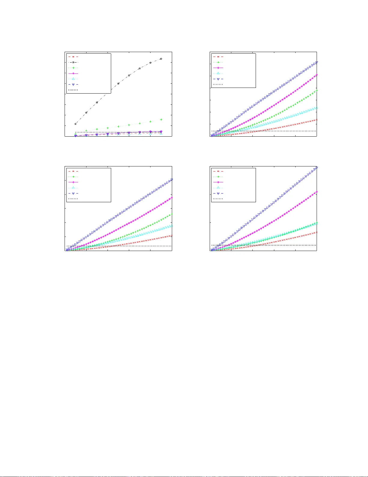
Conditional Gradient Algorithms f or Rank-One Matrix A ppr oximations with a Sparsity Constraint Ronny Luss 1 and Marc T eboull e School of Mathematica l Sciences T el-A vi v Univ ersity , Ramat-A vi v 69978 , Israel email: r onny luss@gmail.co m, teboulle@pos t.tau.ac.il Nov ember 5, 2018 Abstract The sparsity constrained rank- one matrix ap proxim ation prob lem is a dif ﬁcult math ematical opti- mization prob lem which arises in a wide array of useful applications in engineering, machine learning and statistics, and the d esign of algorith ms for this problem has attracted in tensiv e research activities. W e in troduce an algorithm ic fram ew ork, called ConGrad U, that u niﬁes a v ariety of seemingly differ- ent alg orithms that have been der i ved from disparate approa ches, and allows for deriving new schemes. Building on the old and well-known cond itional gradien t algorithm , ConGra dU is a simpliﬁed version with unit step size and yields a generic algor ithm wh ich either is giv en by an analytic form ula or re- quires a very low computatio nal complexity . Mathematical pr operties are systematically developed and numerical experiments are gi ven . Ke ywords : Sparse Principal Component Analysis, PCA, Conditio nal Gradie nt Algorithms, S parse Eigen v alue P roblems, Matrix Approx imations 1 Introd uction The proble m of interes t here is the sparsity constrain ed rank-one matrix approximat ion giv en by max { x T Ax : k x k 2 = 1 , k x k 0 ≤ k , x ∈ R n } , (1) where A ∈ S n is a gi ven real symmetri c matrix, and 1 < k ≤ n is a parameter contro lling the sparsity of x w hich is deﬁned by counting the number of nonzero entrie s of x and denoted using the l 0 notati on: k x k 0 = |{ i : x i 6 = 0 }| . This proble m is also commonly known as the sparse Principal Component A nalysi s (PCA) problem, or as w e refer to it, l 0 -const rained PCA. W ithout the l 0 constr aint, the problem reduces to ﬁnding the ﬁrst prin cipal eige n vector and the co rrespond ing maximal eige n valu e of the mat rix A , i.e., solv es max { x T Ax : k x k 2 = 1 , x ∈ R n } , which is the PCA problem. Suppose A = B T B where B is an m × n mean-centere d data matrix with m samples and n variab les, and denote by v be the principal eigen ve ctor of A , i.e., v solv es the abov e PC A probl em. T hen B v projects the data B to one dimension that maximizes the varian ce of the projec ted data . In general , P CA can be used to reduce B to l < n dimensio ns via the projection B ( v 1 , . . . , v l ) with v i as the i th eigen v ector of A . In addit ion to dimensional ity reductio n, PC A can be used for vis ualizatio n, clustering , and other tasks for 1 Corresponding author 1 data analysis . S uch tasks occur in variou s ﬁelds, e.g., genetics [1 , 27], face recogn ition [16, 38], and signal proces sing [20, 17]. In PCA, the eigen vect or is typically dense, i.e., each component of the eigen vector is nonze ro, and hence the projected varia bles are linear function s of all origina l n v ariable s. In sparse PCA , we restrict the number of variab les used in this linear projection, thereby m aking it easier to interpret the projection s. The additi onal l 0 constr aint ho w e ver makes proble m (1) a dif ﬁcult a nd m athemati cally i nterestin g pro blem which arises in m any scientiﬁc and e ngineer ing application s where v ery lar ge-sca le data sets must be analyz ed and interp reted. Not surprisingly , the search and de velo pment of adequa te algorit hms for solving problem (1) ha ve thus recei ved much attention in the past decad e, and this w ill be discusse d bel ow . But ﬁ rst, we want to make clear the main purpos e of this paper . W e h av e three main goals: • T o dev elop a nove l and v ery simple appro ach to the l 0 -const rained PCA problem (1) as formulated and without any modiﬁcation s, i.e., no relaxations or penaliza tion, which is amenable to dimensions in the hundred s of thousan ds or ev en millions. • T o pres ent a “Fa ther Algorithm”, which we call ConGradU, based on the well-kno wn ﬁrst- order condi- tional gradient scheme, w hich is ver y simple, allows for a rigorous con ve rg ence analysi s, and provid es a family of chea p algori thms w ell-su ited to solving v arious formulatio ns of sparse PCA . • T o provid e a closure and uniﬁcation to many seemingly dispara te approaches recently propose d, and which will be sho wn to be particular realizatio ns of ConGradU. Most curre nt approach es to sparse PCA can b e cate gorized as sol ving one of se veral modiﬁed op timiza- tion probl ems based on penaliza tion, relaxat ions, or both, and include: (a) l 1 -const rained PCA: max { x T Ax : k x k 2 ≤ 1 , k x k 1 ≤ √ k , x ∈ R n } , (b) l 0 -penal ized PCA: max { x T Ax − s k x k 0 : k x k 2 ≤ 1 , x ∈ R n } , (c) l 1 -penal ized PCA: max { x T Ax − s k x k 1 : k x k 2 ≤ 1 , x ∈ R n } , (d) Approximate l 0 -penal ized PCA : max { x T Ax − sg p ( x ) : k x k 2 ≤ 1 , x ∈ R n } , where g p ( x ) ≃ k x k 0 and p controls the approximation , (e) Con vex relaxa tions. These models w ill be presente d in detail in the forthcomin g section, exc ept for appro ach (e) which is not thorou ghly discusse d in this paper (b ut see § 1.1 below). In a nutshell, the original l 0 -const rained PCA problem (1) and the corresp onding modiﬁed problems (a)-(d) abo ve can be written or t ransformed in such a w ay that the y reduce to maxi mizing a con ve x function ov er some compact set C ⊆ R n : ( P ) max { F ( x ) : x ∈ C } . When the p roblem of maximiz ing a linea r function ov er the compact set C can be ef ﬁciently compu ted, or ev en better , can be obtained analytical ly , a very simple and natural iterati ve sche me to consi der for solving (P) is the so-cal led conditi onal gradient algorith m [21, 12] 2 . 2 The conditional gradient scheme is also known as the Frank-W olfe algorithm [15]. The latter was devised to minimize quadratic con vex functions over a bounded polyhedron, whil e t he former was extended mainly to solve con vex mi nimization problems, see Section 3 for more precise details and relev ant references. 2 T o achiev e the goals allud ed to abov e, in this pape r , all dev eloped algorit hms for tackling problem (P) will be based on the conditio nal gradi ent scheme with a unit step size called C onGradU. At this juncture, it is importa nt to notice that Mangasari an [24] seems to ha ve been the ﬁrst work sugge sting and analyzing the condit ional gradien t algorit hm with a unit step size for maximizin g a con ve x function ov er a polyhedr on, in the conte xt of machine learning problems. A co mmon an d inter esting appeal of the resul ting algorith ms is that the y tak e the sha pe of a closed-form iterati ve scheme, i.e., they can be written as x j +1 = S ( Ax j ) kS ( Ax j ) k 2 , j = 0 , 1 , . . . where S : R n → R n is a simple opera tor that can be eithe r written in explicit form or ef ﬁciently co mputed 3 . All prob lems addres sed here are dif ﬁcult nonc on ve x optimizat ion problems and w e mak e n o cl aims with respec t to global optimality; after all, these are difﬁcult proble ms so obtaining cheap soluti ons must hav e some cost which here is a certiﬁca te of global optimality . Moreov er , an important drivin g point is that there is no reaso n to disc ount sta tionary sol utions of noncon ve x prob lems versus globally optimal solutions to con ve x relaxatio ns. For neithe r solution do we ha ve a measur e of the gap to t he optimal so lution of pro blem (1). W e can empirical ly demonstrat e similar soluti on quality , while the noncon ve x methods are orders of magnitud es cheaper to comput e and can be applied to data sets much larger than can be done with any kno w n con ve x relaxatio n. This is in contrast to the w ell-kno wn sparse recov ery proble m, for which there is an eq ui va lence between the dif ﬁ cult co mbinatoria l proble m and the li near prog ram relaxati on w hen t he data matrix satisﬁes certain conditio ns [8]. T o put in perspecti ve the dev elopment and results of this paper , w e ﬁrst discu ss some of the rele vant literatu re that has motiv ated this work. 1.1 Literatur e The literatu re on sparse PCA can be di vided acco rding to th e dif ferent mod iﬁcations discu ssed abov e. Here, we brieﬂy surv ey these approa ches and detail them further in S ection 5. W ith respect to the l 0 -const rained PCA problem (1), thresho lding [7] is perhaps the simplest app roach, ho wev er is known to produ ce poor results . Sparse lo w-rank app roximation s (SLRA) of [39] looks for a more gene ral ( uv T rather than x x T ) sparse approximatio n by taking an approximatio n error lev el as input and determinin g the sparsity lev el k that is require d to satisfy the desired error . Greedy methods [25] are also computati onally ex pensi ve due to a maximum eigen v alue computation at each iteratio n, howe ver an approximat e greedy approach [10] of fers a much cheaper way to deriv e an entire path of soluti ons (for each k = 0 . . . n ) which often sufﬁce . These approa ches are heur istics. The o nly gl obally optimal a pproach to th is formu lation is an e xact searc h method [25] that is applica ble only to extre mely small problems. The l 1 -const rained PCA p roblem is a relaxa tion, or mor e preci sely an upper boun d, to pro blem (1). This proble m was ﬁrst cons idered in [18] and calle d SCoTLAS S (simpliﬁed compone nt techniqu e least absolut e shrink age and selection). It was motiv ated by the LASS O (leas t absol ute selection and shrinka ge operat or) approa ch used in statistics [33] for inducin g sparsity in regressio n. In [34], a true penalty functio n is used to handle the l 1 constr aint and the resultin g pro blem is solv ed as a system of diffe rential equation s (which requir es a smooth ap proximatio n for the l 1 constr aint). While this ap proach was teste d solely on a small 13- dimensio nal data set, we mention it as the only true penalty function approach in the sparse PC A litera ture. 3 In fact, when S is the identity operator, the scheme is nothing else but the well known po wer method to compute the ﬁrst principal eigen vector of the matrix A , see, e.g., [32]. 3 More recen tly , a co mputation ally cheap app roach to l1-co nstrain ed PCA t hat can solve lar ge-scale problems was gi ven by [36]. W e w ill sho w that this scheme is an applic ation of the conditi onal gradient algorit hm. As alre ady expl ained in the introdu ction, we are not inte rested in formu lations that req uire expe nsi ve computa tions. Con ve x relaxations are ei ther semideﬁni te-based or op timize o ver symmetric n × n matrice s, and are, indeed, much more computational ly expensi ve than what we would like to consider here. N e ver - theles s, it is importa nt to br ieﬂy reca ll some of th ese wo rks. In [1 1], d’Aspr emont et a l. introduc ed a con ve x relaxa tion to l 1 -const rained PCA using semideﬁnite pro gramming, ho we ver this formula tion can only be solv ed on very small dimensions ( < 100 ). T his was the ﬁ rst approa ch with con vex optimization to any sparse PCA modiﬁcation and moti va ted a con vex relaxati on for l 1 -penal ized PCA for which better algo- rithms were gi ven. Anothe r approac h for l 1 -const rained PC A in [22] solves a dif ferent con ve x relaxation ov er S n based on a varia tional repre sention of the l 1 ball ( this relaxation turne d out to be the dual of the semideﬁnit e relax ation in [11]). This was the ﬁrst con ve x relaxati on for l 1 -const rained PCA amenable to a medium number of dimension s (1000-20 00). W e nex t turn to penalized sparse PCA where the sparsi ty-induc ing term appears in the objecti ve func- tion. Sev eral approac hes are known for l 0 -penal ized PCA . The heur istic giv en in [39] is extend ed in [40] to this penalize d v ersion of PCA. In [10], the problem is reformulated as an equi va lent con vex maximization proble m to which a semideﬁnite relax ation is applied, ho wev er , as mentione d abo ve, solv ing such problems is too computation ally expe nsi ve. More recen tly , [19] deri ved the same con ve x maximization problem (in a dif ferent manner) and prop osed a ﬁ rst-or der gradient-ba sed algorithm which is identical to ConGradU. Another con vex maximization repres entation was very recently presented in [31], whereb y a speciﬁc pa- rameteriz ed conca ve approx imation is used to replace the l 0 term, and the resultin g problem was solved by an iterati ve scheme called the minorizati on-maximiza tion technique, which is, in fact, a speciﬁc instance of ConGradU. The l 1 -penal ized P CA problem can be solved by a con ve x relaxat ion as shown in [11], b ut is amenable to only a medium number of dimensions. In [41], Zhou et al. conside red a reformulatio n of PC A as a two v ariable re gressio n problem to whi ch an l 1 penalt y is add ed for one of t he v ariables. While their a pproach is amenable to lar ger problems, it is not exac tly l 1 -penal ized PCA and is s till more computat ionally expensi ve (cf. Section 5.4) than other approa ches we w ill discuss. Recently , [19] reformul ated l 1 -penal ized PCA as an equi va lent con vex maximizati on problem (as w ith their l 0 -penal ized approach) that is also solv ed by the condit ional gradien t algorit hm. As disc ussed abo ve, the conditional gradient alg orithm has prev iously been app lied to sparse PCA in v arious forms, so we now put the contrib utions of the abov e works into perspecti ve. The works of [36, 29] detail the ir iterati ve schemes (withou t any gene ral algorith m) spe ciﬁcally for sparse P CA. [31] details a genera l algorithm, similar to ConGradU, but meant for maximizing the dif ference of con ve x functions ov er a con ve x set . While m aximizin g a con v ex function is a subset of this algorithm, ConGradU, as detailed in Section 3, allo w s for noncon ve x sets. [19] is the only pre viousl y kno wn work that details a general algori thm for maximizing a con vex function o ver a compact (possib ly noncon vex) set. Inde ed, the ﬁ rst- order algorit hm prop osed in [19] (labeled Algorithm 1 therein) is identic al to what w e term the ConGradU algori thm, howe ver it is not recogniz ed as the condi tional gra dient algorithm. As noti ced in [19], both the l 0 and l 1 -penal ized PCA algori thms they ha ve pro posed were earlier stated in [29], subject to sligh t modiﬁcatio ns, who look for a general rank- one approximati on (i.e., uv T rather tha n xx T ); ho wev er , no con ver gence results were stated in [29]. 4 1.2 Outline W e provi de computa tionally simple approaches to both const rained and penaliz ed ver sions of sparse PC A. It is important to recognize that all algorith ms here are schemes for noncon ve x problems; we pay the price of no global optimality criteri on and gain in amenab ility to problem sizes that con vex relaxati ons can not handle . In Section 2, we deﬁne the proble ms of interes t and some of their properties . Sec tion 3 recalls some basic optimality results for maximizing a con ve x function over a compact set. W e then detail ConGradU, a speciﬁc conditio nal gradi ent scheme with unit step size, and establis h its con ver gence properties . Section 4 pro vides a mathematic al toolbox provin g a series of propositio ns that are used to de velo p the kno wn cheap algori thms mentione d above , as w ell as for deri ving new schemes. These propositi ons are simple and easy to pro ve so we belie ve it beneﬁts the reader to go through these tools ﬁ rst. Section 5 then detai ls the algor ithms for a ll v ersions of spar se PCA. W e s tart with a si mple algo rithm for the true l 0 -const rained PCA problem (1). T o the author’ s kno w ledge, this is the ﬁrst av ailable scheme that directl y approac hes this probl em, is amenable to large -scale probl ems and prove n to con ver ge to a stationa ry point of problem (1). While the l 0 constr aint is a difﬁcult nonsmoo th and noncon ve x constrain t, we need not look for ways aroun d thi s con straint, and rather we approac h the gi ven probl em as is. The basis for our approach is the simple, yet surprising, result (cf. Section 4 ) that while m aximizin g a quadrat ic function ov er the l 2 unit ball with an l 0 constr aint is a difﬁcult problem, maximizing a linear function ove r the same nonco n vex set is simple and can be solve d in O ( n ) time. An important aspect of the new l 0 -const rained PCA algorithm is that no parameters need be tuned in order to obtai n a stationa ry point that has the exact desire d sparsity 4 . The se cond main part of Sec tion 5 focu ses on all afor ementioned iterati ve schemes which ha ve been propose d in the literatur e. Building on the results of Section 4, we show that all these schemes can directly be obtained as a particular realiz ation of ConGradU, or of some v ariant of it, thus providin g a unifyi ng frame work to v arious seemingly dif ferent algorithmic approache s. Section 6 provides ex perimenta l res ults and demons trates the ef ﬁcienc y of many of the m ethods we ha ve re vie wed on larg e-scale problems. W e show that the y all giv e comparable solutions, i.e., very similar k -sparse solutions , with the advan tage of l 0 -const rained PCA being that the k -sparse solution is direc tly obtain ed at a lo wer computatio nal cost. S ection 7 ends with concl uding remarks and brieﬂy shows ho w to use the same tools to de velop simple algorithms for related sparsity constrain ed problems. 1.3 Notation W e write S n ( S n + , S n ++ ) to denote the set of symmetric (positi ve-semid eﬁnite, positi ve-de ﬁnite) matrices of size n and R n ( R n + , R n ++ ) to denote the set of (nonne gati ve, strictly posit iv e) real v ectors of size n . The vec tor e is the n -ve ctor of ones . Giv en a vecto r x ∈ R n , k x k 2 = ( P i x 2 i ) 1 2 deﬁnes the l 2 norm, k x k 0 deﬁnes the card inality of x , i.e., the number of non zero entri es of x and u sually cal led her e th e l 0 norm 5 , an d k x k ∞ = max ( | x 1 | , . . . , | x n | ) . Gi ven a matrix X ∈ S n , k X k ∞ = max i,j X i,j and k X k F = ( P i,j X 2 i,j ) 1 2 . For a vecto r x ∈ R n , | x | denotes the ve ctor with i th entry | x i | , sgn ( x ) denotes the v ector with i th entry -1,0,1 if x i < 0 , x i = 0 , x i > 0 , and x + denote s the v ector with i th entry max ( x i , 0) . For a v ector x ∈ R n , diag ( x ) denotes the diago nal matrix with x on its diago nal. Fo r an y nonze ro inte ger n , denote the set { 1 , . . . , n } as [ n ] . Let I n denote the identity matrix in dimen sion n . Let C 1 denote the space of 4 All other algorithm based on mo diﬁcations can be used to obtain a d esired sparsity as well, ho weve r parameters must be tune d accordingly . 5 W e note an ab use of terminology because k x k 0 is not a true norm since it is not positiv ely homogenous . 5 once continu ously dif ferentia ble functions on R n . G i ven an optimization problem (P), we use argmax( P ) to deno te its optimal solution s set. 2 Pr oblem F ormulations This section describes the relation ship between l 0 -const rained PCA and the v arious modiﬁed sparse PCA proble ms that are discuss ed through out the paper , as well as certain proper ties. 2.1 The Original Optimization Model W e start with some useful and elementary propert ies of the l 0 -const rained PCA probl em. The l 0 -constra ined P CA Pro blem Giv en a symmetric m atrix A ∈ S n and sparsity lev el k ∈ [1 , n ] , the main problem of interest is to solve the l 0 -const rained PCA probl em (i.e., the sparse eigen value problem): ( E ) max { x T Ax : k x k 2 = 1 , k x k 0 ≤ k , x ∈ R n } . (2) In most applica tions, A is the cov ariance matrix of some data m atrix B ∈ R m × n such that A = B T B and hence is positiv e semideﬁnite. The latter fact will be exp loited in reformulati ons of the problem describ ed belo w . In fac t, as is very well-kno wn, since problem (E ) is constr ained by the unit sphere , without loss of genera lity (see e.g ., [10, 11, 19]) we can a lway s assu me that A is po siti ve semid eﬁnite sinc e we clearly ha ve max x ∈ R n { x T A σ x : k x k 2 = 1 , k x k 0 ≤ k } = max x ∈ R n { x T Ax : k x k 2 = 1 , k x k 0 ≤ k } + σ, with σ > 0 such that A σ := A + σ I n ∈ S n ++ , i.e., w ith respect to optimal objecti ve values w e are solving the same probl em. The next result furthermore states that w e can relax the sphere constrai nt to its con v ex counterp art, the unit ball, namely we consid er the problem ( E σ ) max { x T A σ x : k x k 2 ≤ 1 , k x k 0 ≤ k , x ∈ R n } and also show that problems ( E ) and ( E σ ) are equiv alent and admit the same set of optimal solutions . The simple proof is omitted. Lemma 1 F ix an y σ > 0 such that A σ ∈ S n ++ . Then, (a) max { x T A σ x : k x k 2 ≤ 1 , k x k 0 ≤ k } = max { x T Ax : k x k 2 = 1 , k x k 0 ≤ k } + σ. (b) argmax( E ) = argmax( E σ ) . Needless to say that both problems ( E ) and ( E σ ) remain hard nonc on vex problems as they consist of maximizing a con vex (strongly con vex) fun ction over a compact set, and clearly the possibility of using the con ve x relaxation { x : k x k 2 ≤ 1 } instead of the noncon vex unit sphere constraint does not change the situati on. Howe ver , it is useful to kno w that either one of these constrain ts can be used when tacklin g the proble m, and this will be done through out the rest of the paper without any f urther mentioning . Through out the pap er , ( E ) will be refer red to as the l 0 -const rained P CA problem, and A alw ays de notes a symmetric matrix while A σ will denote a symmetric positi ve deﬁnite m atrix. W e no w consid er the other formulat ions that will be analyz ed. 6 2.2 Modiﬁed Optimization Models As mentioned in the introductio n, most approach es to sparse P CA solv e one of the follo wing modiﬁed proble ms. The ﬁrst va riation is a relaxatio n based on the relation k x k 1 ≤ p k x k 0 k x k 2 ∀ x ∈ R n (3) which follo ws from the Cauchy-Sch warz inequalit y . The hard l 0 constr aint in probl em (2) is repl aced by an l 1 constr aint, resultin g in The l 1 -constra ined P CA Pro blem max { x T Ax : k x k 2 ≤ 1 , k x k 1 ≤ √ k , x ∈ R n } , (4) which tha nks to inequality (3) is an uppe r bound to the origin al l 0 -const rained PC A problem. T wo other v ariation s are based on penalization s of the l 0 and l 1 constr aints of the abov e formulation s. Note that the penali zed terminolo gy is dif ferent from the usual one used in optimizati on, and here is used to mention that it rather optimizes a tradeof f between ho w good and ho w sparse the approximat ion is. W e ﬁrst penalize the l 0 constr aint in problem (2), resultin g in The l 0 -penalized PCA Pr oblem max { x T Ax − s k x k 0 : k x k 2 ≤ 1 , x ∈ R n } , (5) where s > 0 is a par ameter that must be tuned to ac hie ve the tru ly desired sparsi ty lev el at which k x k 0 = k . Ho wev er , to av oid the tri vial optimal solution x ∗ ( s ) ≡ 0 , the parameter s must be restric ted. First recall the well-kno wn norm relatio ns k x k ∞ ≤ k x k 2 ≤ k x k 1 , ∀ x ∈ R n . (6) Using the H ¨ older ineq uality 6 , combin ed with inequa lities (3) and (6), it follo ws that x T Ax − s k x k 0 ≤ k A k ∞ k x k 2 1 − s k x k 0 ≤ ( k A k ∞ − s ) k x ∗ k 0 , for all x feasibl e for problem (5). T hus, to a void the tri vial solution, it is assumed that s ∈ (0 , k A k ∞ ) . Note that while s ≥ k A k ∞ necess arily implies the t riv ial so lution, taking s < k A k ∞ does not guaran tee we a vo id it, b ut only gi ves a particul ar bound. Like wise, a penalized version of the l 1 -const rained PCA probl em (4) yields The l 1 -penalized PCA Pr oblem max { x T Ax − s k x k 1 : k x k 2 ≤ 1 , x ∈ R n } . (7) Note that, as in problem (5), we need to restric t the v alue of the parameter s in order to av oid the tri vial soluti on. Again, using the H ¨ older ineq uality and (6), it is easy to see that x T Ax − s k x k 1 ≤ ( k A k F − s ) k x ∗ k 1 , for all x feasib le for problem (7 ), and hen ce it is assumed that s ∈ (0 , k A k F ) . 6 For any u , v ∈ R n , the H ¨ older inequality states that |h u, v i| ≤ k u k p k v k q , where p + q = pq , p ≥ 1 . 7 Again, n ote tha t the formulat ed penalized /relax ed problems remain hard n oncon v ex maximizati on prob- lems desp ite the con ve xity of their con straints. In fact , l 0 -penal ized PCA and the l 1 -penal ized ver sion share an additiona l difﬁcul ty in that their objecti ves are neither conca ve nor con vex. In Sections 5.3 and 5.4, we sho w ho w this dif ﬁculty is overc ome. The Appr oximate l 0 -penalized PCA Pr oblem The last approac h f or solving problem (2) in volv es appr oximating the l 0 norm in the objecti ve of l 0 -penal ized PCA. The idea of approximat ing the l 0 norm by some nicer cont inuous func tions naturally emer ged from ver y well-kno wn mathema tical approximatio ns of the step and sign function s (see, e.g., [6]). Indeed, it is easy to see that for an y x ∈ R n , one can write k x k 0 = n X i =1 sgn ( | x i | ) . Thus, formally , we want to replac e the problematic expr ession sgn ( | t | ) by some nice r function and consi der an approxi mation of the form k x k 0 = lim p → 0 n X i =1 ϕ p ( | x i | ) , where ϕ p : R + → R + is an approp riately chosen smooth funct ion. Here, we consider the class of smooth conca ve functions which are m onoto ne increasing and normaliz ed such that ϕ p (0) = 0 , ϕ ′ p (0) > 0 . This suggest s to approx imate problem (5) by considering for p, s > 0 the follo wing approxi mate maxi- mization proble m: max { x T Ax − s n X i =1 ϕ p ( | x i | ) : k x k 2 ≤ 1 , x ∈ R n } . (8) Approxima tions of the l 0 norm hav e been consider ed in variou s app lied conte xts, for instan ce in the machine learnin g literat ure, see, e.g., [24, 35]. There exis t se veral possible choices for the function ϕ p ( · ) that approximate the step funct ion, and for details the reader is referred to the classic book by Brace well [6, C hapte r 4]. For illustration , here we giv e the follo wing example s as well as their graphical representa tion in Figure 1 (left). Example 2 Concave functions ϕ p ( · ) , p > 0 (a) ϕ p ( t ) = (2 /π ) tan − 1 ( t/p ) , (b) ϕ p ( t ) = log (1 + t/p ) / log (1 + 1 /p ) , (c) ϕ p ( t ) = (1 + p/t ) − 1 , (d) ϕ p ( t ) = 1 − e − t/p . The last e xample (d) was successfully used in the conte xt of machine lear ning by Mang asarian [2 4], and gi ves ϕ p ( | t | ) = 1 − e − p | t | = ( 0 if t = 0 > 0 if t 6 = 0 . (9) 8 0 0.5 1 1.5 2 0 0.2 0.4 0.6 0.8 1 (2/pi)arctan(t/p) log(1+t/p)/log(1+1/p) 1/(1+p/t) 1−exp(−t/p) P S f r a g r e p l a c e m e n t s Approx imations ϕ p ( t ) with p = . 05 ϕ p ( t ) t 0 0.5 1 1.5 2 0 0.2 0.4 0.6 0.8 1 p=.05 p=.5 p=1 p=5 P S f r a g r e p l a c e m e n t s Approx imation as p → 0 1 − e − t/p t Figure 1: T he left plot sho ws four concave fun ctions ϕ p ( t ) th at can be used to approximate k x k 0 ≈ P n i =1 ϕ p ( | x i | ) f or ﬁxed p = . 05 . The right plot shows how the c oncave approx imation 1 − e − t/p conv erges to the indicator function as p → 0 . A nice feature of this exa mple is that it also lower bou nds the l 0 norm, namely , we ha ve n X i =1 ϕ p ( | x i | ) ≤ k x k 0 , ∀ x ∈ R n . See Figure 1 (right ) for its beha vior for var ious valu es of p . All proble ms listed in this sectio n, as well as se veral other equi val ent refo rmulations that will be de- ri ved in Section 5, will be solv ed by ConGradU, a condition al gradient algorithm with unit step size for maximizing a con ve x function over a c ompact set which is described next. 3 The Conditional Gradient Algorithm 3.1 Backgr ound The conditiona l gradien t algo rithm, is a well-kn own and simple gradie nt algorithm, see, e.g., [21, 12] and the b ook [4] for a gene ral ov erview of th is method as well as mo re re ferences . Note th at this algorithm dates back to 195 6, and is also kno w n as the Fran k-W olfe algorithm [15] that was orig inally proposed for solvin g linearl y constrained quadratic programs. The condi tional gradien t algorithm is presente d here for maximization problems because of our interes t in the sparse PCA problem. W e ﬁrst recall the cond itional grad ient algo rithm for maximizing a continu ously dif ferent iable function F : R n → R over a none mpty compact con vex set C ⊂ R n : max { F ( x ) : x ∈ C } . (10) The condi tional gradien t algorithm generates a sequence { x j } via the iteration: x 0 ∈ C, x j +1 = x j + α j ( p j − x j ) , j = 0 , 1 , . . . 9 where p j = argmax {h x − x j , ∇ F ( x j ) i : x ∈ C } , (11) and w here α j ∈ (0 , 1] is a stepsize that can be determined by the Armijo or limited maximization rule [4]. It can be sho wn that ev ery limit point of the sequenc e { x j } generate d by the condition al gradient algorithm is a stationa ry point. Furthermore , under var ious additional assumpti ons on the function F and/or the set C (e.g., stro ng con ve xity of the func tion F and/or of the set C ), rate o f con ver gence results can b e estab lished, see in partic ular the work of Dunn [13] and refer ences therein. Clearly , the condition al gradien t algorithm becomes attract iv e and simple when its main computationa l step (11) can be perfor med ef ﬁciently , e.g., when C is a boun ded polyhed ron it reduces to solving a linear progra m, or e ven bette r when it can be solved analy tically . 3.2 Maximizing a Con vex Function via ConGradU As we shall see belo w , all potential refor mulations of the spars e PCA problem w ill lead to maximizin g a con ve x (poss ibly nonsmoot h) functio n ov er a compact (possibl y noncon ve x) set C ⊂ R n . It will be shown that, for such a class of problems, the conditional gradie nt alg orithm will reduce to a ver y simple iterati ve scheme. First we recall some basic deﬁnitions and propert ies rele v ant to m aximizin g con vex function s. Let F : R n → R be con ve x, and C ⊂ R n be a n onempty compact set. Throughout , we assume tha t F is not consta nt on C . W e den ote by F ′ ( x ) any su bgradie nt of the con vex function F at x which satisﬁes F ( v ) − F ( x ) ≥ h v − x, F ′ ( x ) i , ∀ v ∈ R n . (12) The set of all subgra dients of F at x is the subdif ferenti al of the function F at x , deno ted by ∂ F ( x ) , i.e., ∂ F ( x ) = { g : F ( v ) ≥ F ( x ) + h v − x, g i , ∀ v ∈ R n } , which is a closed con ve x set. When F ∈ C 1 , the subdif ferential reduces to a singleton which is the gradient of F , that is ∂ F ( x ) = {∇ F ( x ) } , and (12) is the usual gradient inequality for the con vex function F . In the follo wing, w e use the notatio n F ′ ( · ) to refer to either a gradient or subgradie nt of F ; the context will be clear in the rele v ant situation. The ﬁrst result r ecalls two useful properties when max imizing a con ve x function (se e [28, Sectio n 32]). Pro position 3 Let F : R n → R be con ve x, S ⊂ R n be an arbitr ary set and let con v ( S ) denote its con ve x hull. Then, (a) sup { F ( x ) : x ∈ con v ( S ) } = su p { F ( x ) : x ∈ S } , wher e the ﬁr st supr emum is attained only if the second is attaine d. (b) If S ⊂ R n is close d with nonempty bounda ry bd ( S ) , and F is bounded above on S , then su p { F ( x ) : x ∈ S } = sup { F ( x ) : x ∈ bd ( S ) } . The next result giv es a ﬁrst-order optimality criterion for maximizing a con vex function F ov er a com- pact set C ∈ R n . It uses property (a) of Propositi on 3 and follo ws from [28, Corollary 32.4.1]. Pro position 4 Let F : R n → R be con ve x. If x is a local maximum o f F over the no nempty compact set C , then ( F O C ) h v − x, F ′ ( x ) i ≤ 0 , ∀ v ∈ C. (13) 10 When F ∈ C 1 , a point x ∈ C sat isfying the ﬁrst-order optimality criteria (FOC) (13 ) w ill be referred as a stationa ry point, othe rwise, when F is con vex nonsmoo th, we will say that the poi nt x ∈ C satisﬁes (FOC). W e are no w ready to state the algorithm. It turns out that when the functio n F is con ve x and quadratic, we can al so eliminate the nee d for ﬁnding a step s ize and consi der the condition al gradient algori thm with a ﬁxed unit step size and still preserve its con ver gence properties . This simpliﬁed version of the cond itional gradie nt algorith m will be used through out the paper and referred to as ConGradU. Algorithm 1 ConGradU – Conditional Gradient Algorithm with Unit Step Size Require : x 0 ∈ C 1: j ← 0 , 2: while stoppi ng criteria do 3: x j +1 ∈ argmax {h x − x j , F ′ ( x j ) i : x ∈ C } 4: end while 5: r eturn x j T o analyze ConGradU, in what follo w s, it will be con venien t to introduce the quantity γ ( x ) := max {h v − x, F ′ ( x ) i : v ∈ C } (14) for any x ∈ R n . Since C is co mpact, this quantity is w ell-de ﬁned and admits a global maximizer u ( x ) ∈ argmax {h v − x, F ′ ( x ) i : v ∈ C } , and thus, we ha ve γ ( x ) = h u ( x ) − x, F ′ ( x ) i . In te rms of the ab ov e deﬁned qua ntities, we thus ha ve that x ∗ satisﬁes (FOC) is equ iv alent to say ing that x ∗ is a global maximizer of ψ ( v ) = h v − x ∗ , F ′ ( x ∗ ) i , i.e., x ∗ ∈ argmax {h v − x ∗ , F ′ ( x ∗ ) i : v ∈ C } = u ( x ∗ ) . Thus the C onGradU algorithm is nothing else b ut a ﬁxed point scheme for the map u ( · ) , and simply reads as x 0 ∈ C, x j +1 = u ( x j ) , j = 0 , 1 , . . . . Lemma 5 Let F : R n → R be con ve x, C ⊂ R n be nonempty and compact, and let γ ( x ) be given by (14). Then, (i) γ ( x ) ≥ 0 for all x ∈ C . (ii) F or a ny v ∈ C and any x ∈ R n , F ( u ( x )) − F ( x ) ≥ γ ( x ) ≥ h v − x, F ′ ( x ) i . Pro of. T he proof of (i) and the rig ht ine quality of (ii) follo ws immediat ely fro m the deﬁnition o f γ ( x ) , while the left inequa lity in (ii) follo ws from the subgradi ent inequality for the con vex functio n F : F ( u ( x )) − F ( x ) ≥ h u ( x ) − x, F ′ ( x ) i = γ ( x ) . W e are ready to state the con ver gence properties of C onGradU. 11 Theor em 6 Let F : R n → R be a con vex function and let C ⊂ R n be nonempty compact. Let { x j } be the sequen ce gene rated by the algorith m ConGradU . Then the following statement s hold: (a) the sequenc e of functio n values F ( x j ) is monoto nically incr easing and lim j →∞ γ ( x j ) = 0 . (b) If for some j the iterat e x j satisﬁ es γ ( x j ) = 0 , then the algorithm stops with x j satisfy ing (FOC). Oth- erwise the algori thm gen erate s an inﬁnite sequence { x j } w ith stric tly incr easing function values { F ( x j ) } . (c) Mor eover , if F is continu ously dif fer entiable , then eve ry limit point of the sequenc e { x j } con ver ges to a statio nary point. Pro of. By deﬁnition of the iterat ion of ConGradU, using our notations, the seque nce { x j } is well deﬁned via x j +1 ∈ u ( x j ) , ∀ j = 0 , 1 . . . . In vok ing Lemma 5, we obtain 0 ≤ γ ( x j ) ≤ F ( x j +1 ) − F ( x j ) , ∀ j = 0 , 1 , . . . , sho w ing that the seq uence { F ( x j ) } is monotone inc reasing. Summing the inequal ity abov e for j = 0 , . . . , N − 1 , we ha ve N − 1 X j =0 γ ( x j ) ≤ F ( x N ) − F ( x 0 ) . Since C is compact and F ( · ) is continu ous, we also ha ve F ( x N ) ≤ m ax { F ( x ) : x ∈ C } := F ∗ , and thus it fo llo ws from th e abo ve inequ ality that P N − 1 j =0 γ ( x j ) ≤ F ∗ − F ( x 0 ) , a nd hen ce the n onne gati ve series P ∞ j =0 γ ( x j ) is con ver gent so that γ ( x j ) con ver ges to 0. Now , since γ ( x j ) ≥ 0 for all j = 0 , . . . , then if for some j the iterate x j is su ch that γ ( x j ) = 0 then the proced ure stops at ite ration j with x j satisfy ing (FOC ). Otherwise, γ ( x j ) > 0 and the iteration generates an inﬁnite sequence w ith F ( x j +1 ) > F ( x j ) . In the latter case, assuming no w that F ∈ C 1 , we will no w prov e the last stateme nt of the theorem. Since C is compact, the sequence { x j } ⊂ C is bounded. Passing to subsequenc es if necessary , for any limit point x ∞ of { x j } we thus ha ve x j → x ∞ . W ithout loss of generality w e let u ( x j ) → ¯ u . Using the fac ts γ ( x j ) = h u ( x j ) − x j , F ′ ( x j ) i and h v − x j , F ′ ( x j ) i ≤ h u ( x j ) − x j , F ′ ( x j ) i , ∀ v ∈ C, and sin ce γ ( x j ) → 0 and F ∈ C 1 , passi ng to the limit o ver ap propriat e subseque nces in the abov e relations, it follo ws that h ¯ u − x ∞ , F ′ ( x ∞ ) i = 0 and h v − x ∞ , F ′ ( x ∞ ) i ≤ h ¯ u − x ∞ , F ′ ( x ∞ ) i , ∀ v ∈ C , and hence h v − x ∞ , F ′ ( x ∞ ) i ≤ 0 , ∀ v ∈ C , sho wing that x ∞ is statio nary . Remark 7 (a) F or the case of con vex F and bounded polyhedr on C , as noted in the intr oduction, Man- gasar ian [24] seems to have been the ﬁrst work sugg esting the possibilit y of using a uni tary step size in the con ditiona l gra dient sch eme and pr o ved that the algorithm gener ates a ﬁnite sequ ence (thanks to the polyhe dral ity of C ) that termina tes at a stati onary point. (b) V ery r ecentl y , the use of a unit ary stepsize in the condition al gradient sch eme was re disco ver ed in [19] with C being an arbitra ry compact set, which is iden tical to Algorithm 1. (c) The pr oof of Theor em 6 is patterned after the one given in [24 ]. Note tha t par t (a) also follows fr om [19] as well. Further mor e, under str ong er assumptions on F and C , [ 19, Theor em 4] also establis hed a stepsize con ver genc e ra te giving an upper estimate on the number of iterat ions the algorithm take s to pr oduce a step of small size. (d) Fin ally , as kindly pointed out by a ref er ee, the pr oof of con ver gence could also pr obably be derived by using the gen eral appr oac h devel oped in the classical m ono grap h of Zangwill [37]. 12 W e end this s ection with a part icular realizatio n of ConGradU for an intere sting class of proble ms giv en as ( G ) max x { f ( x ) + g ( | x | ) : x ∈ C } where f : R n → R is con vex , g : R n + → R is con ve x differe ntiable and m onoto ne decreasing 7 , C ⊆ R n is a compact set. Our interest for this form is m ainly driv en by and is particul arly useful for hand ling the case of the approx imate l 0 -penal ized problem (cf. Section 5 .3), whic h preci sely has the form of this op timization model with adequate choice of the kerne l ϕ p that can be used to approximat e the l 0 norm (cf. Section 2). It will also allo w for de vel oping a nov el simple scheme for the l 1 -penal ized problem (cf. Section 5.4). Note that under the stated assumptio ns for g , the compositio n g ( | x | ) is not necessarily con ve x and thus ConGradU cannot be applied to problem (G). Howe ver , thank s to the component wise monotonic ity of g ( · ) , it is easy to see that problem (G) can be recas t as an equi valen t problem with additional constraints and v ariables as follo w s: ( GG ) max x,y { f ( x ) + g ( y ) : | x | ≤ y , x ∈ C } . Note that, wit hout loss of genera lity , an addit ional u pper bou nd c an be imposed on y in order to enforc e co m- pactne ss of the feas ible re gion of problem (GG) (e.g., by setting the uppe r bo und o n y as y c := argmax {| x | : x ∈ C } ), b ut this need no t be compute d in order to esta blish our f ollo wing result. Clearly , the ne w object iv e of (GG) i s no w co n vex i n ( x, y ) and thus we can a pply Con GradU. W e sho w belo w that th e main iteration in that cas e leads to an a ttracti ve weighted l 1 -norm maximiz ation proble m, which, in turn, as sho wn in Sectio n 4 can be solved in closed form for the cases of interes t, namely when C is the compact set described by the unit spher e or unit ball. Pro position 8 The algorith m ConGradU applie d to pr oblem (GG ) gen erate s a sequence { x j } by solving the weighted l 1 -norm maximizatio n pr oblem x 0 ∈ C, x j +1 = argmax {h a j , x i − X i w j i | x i | : x ∈ C } , j = 0 , . . . , (15) wher e w j = − g ′ ( | x j | ) > 0 and a j = f ′ ( x j ) ∈ R n . Pro of. Appl ying ConGradU to the con ve x funct ion H ( x, y ) := f ( x ) + g ( y ) , with y 0 = | x 0 | , x 0 ∈ C we obtain , ( x j +1 , y j +1 ) = argmax x,y {h x − x j , f ′ ( x j ) i + h y − y j , g ′ ( y j ) i : x ∈ C , | x | ≤ y } = argmax x ∈ C  h x − x j , f ′ ( x j ) i + max y {h y − y j , g ′ ( y j ) i : | x | ≤ y }  = argmax x ∈ C  h x − x j , f ′ ( x j ) i + h| x | − y j , g ′ ( y j ) i  , 7 By monotone decreasing, we mean componentwise, i.e., each component of g ′ ( · ) the gradient of g is such that g ′ i ( · ) i < 0 ∀ i ∈ [ n ] . 13 where the last max computation with respect to y uses the fact that g ′ is m onoto ne decrea sing. It is als o cl ear that, gi ven the initializa tion y 0 = | x 0 | and y j +1 = argmax {h y , g ′ ( y j ) i : | x j +1 | ≤ y } , w e hav e y j = | x j | for all j = 0 , 1 , . . . Omitting const ant terms, the last iteratio n can be simply re written as x j +1 = argmax x ∈ C {h x, f ′ ( x j ) i + h| x | , g ′ ( | x j | ) i} , which with w j := − g ′ ( | x j | ) > 0 prov es the desired result stated in (15). 4 A Simple T oolbox for Bui lding Simple Algorithms The algorithms discussed in this paper are based on the fa ct that the l 0 -const rained PCA problem as well as many of the penalize d and constrai ned l 0 and l 1 optimiza tion prob lems that are solved by the proposed condit ional gradient algorithm ha ve iterations that either hav e closed form solutio ns or are easily solv able. Speciﬁcally , the main step of ConGradU m aximizes a linear function over a compact set, and the followin g lemmas and propos itions sho w that for certain compact sets (e.g { x ∈ R n : k x k 2 = 1 , k x k 0 ≤ k } and { x ∈ R n : k x k 2 = 1 , k x k 1 ≤ k } ), these subprobl ems are easy to solv e. In addition , proposition s are gi ven that will be used to reformulat e (in Section 5) prob lems such as l 0 and l 1 -penal ized P CA, which ha ve neither con ve x nor conca ve objecti ves , to problems that maximize a con ve x objecti ve function. The propo sitions for maximizing linear functions ov er compact sets can then be used in ConGradU as applied to the reformulated l 0 and l 1 -penal ized PCA probl ems. Combine d with the condit ional gradient algori thm discussed abo ve, these propositio ns are the only tools required thro ughout the remainde r of the paper . W e start with an obvio us but very use ful lemma that is used in all of the follo wing propositio ns. Lemma 9 Given 0 6 = a ∈ R n , max {h a, x i : k x k 2 = 1 , x ∈ R n } = max {h a, x i : k x k 2 ≤ 1 , x ∈ R n } = k a k 2 , with maximizer x ∗ = a/ k a k 2 . Pro of. Immediate from Cauchy-Sch warz inequality . The follo wing propos itions make use of the follo wing operat or: Deﬁnition 10 G iven any a ∈ R n , deﬁn e the oper ator T k : R n → R n by T k ( a ) := argmin x {k x − a k 2 2 : k x k 0 ≤ k , x ∈ R n } . This ope rator is thus the best k -sparse app roximatio n of a gi ven vec tor a . Despite the noncon vexity of the constraint, it is easy to see that ( T k ( a )) i = a i for the k lar gest entries (in absolute va lue) of a and ( T k ( x )) i = 0 oth erwise. In case the k large st entries are not uniqu ely deﬁned, we select the smalles t possib le indices. In other words , w ithout los s of gener ality , w ith a ∈ R n such | a 1 | ≥ . . . ≥ | a n | , we ha ve ( T k ( a )) i =  a i , i ≤ k ; 0 , otherwis e . 14 Computing T k ( · ) only require s determining the k th lar gest number of a vecto r of n numbers which can be done in O ( n ) time [5] and zeroing out the proper compone nts in one more pass of the n numbers. The next proposit ion is an extensi on of L emma 9 to l 0 -const rained problems. T his is the simple result that maximiz ing a linea r function ov er the nonco n vex set { x ∈ R n : k x k 2 = 1 , k x k 0 ≤ k } is equally simple and can be solv ed in O ( n ) time. Pro position 11 Given 0 6 = a ∈ R n , max x {h a, x i : k x k 2 = 1 , k x k 0 ≤ k , x ∈ R n } = k T k ( a ) k 2 (16) with solut ion obtain ed at x ∗ = T k ( a ) k T k ( a ) k 2 . Pro of. By Lemm a 9, the optimal value of proble m (16) is q P i ∈I a 2 i for some subset of indice s I ⊆ [ n ] with |I | ≤ k . The set I that m aximizes this val ue clearly conta ins the indices of the k larges t elements of the vect or | a | . Thus, by deﬁnit ion of T k ( a ) , solvin g problem (16) is equi v alent to solving max x {h x, T k ( a ) i : k x k 2 = 1 , x ∈ R n } from which the result follo ws by Lemma 9. Another vers ion of this result giv es the solution with a squared objecti ve. Pro position 12 Given a ∈ R n , max x {h a, x i 2 : k x k 2 = 1 , k x k 0 ≤ k , x ∈ R n } = k T k ( a ) k 2 2 with solut ion obtain ed at x ∗ = T k ( a ) k T k ( a ) k 2 . Pro of. Notice that the optimal objecti ve v alue in Propositi on 11 is nonne gati ve, and hence the squared object iv e va lue here does not change the optimal solution to the proble m w ith linear objecti ve. The result follo ws. The abo ve prop ositions w ill serv e to deriv e the no vel sche mes giv en in Section 5. The next resu lt is a modiﬁcation of Proposition 12. It sho w s that the l 0 -penal ized versio n of maximiz ing a squared linear functi on yields a closed-f orm solution. Pro position 13 Given a ∈ R n , s > 0 , max x {h a, x i 2 − s k x k 0 : k x k 2 = 1 , x ∈ R n } = n X i =1 ( a 2 i − s ) + is solve d by x ∗ i = a i [ sgn ( a 2 i − s )] + q P n j =1 a 2 j [ sgn ( a 2 j − s )] + . 15 Pro of. Assume without loss of general ity that | a 1 | ≥ . . . ≥ | a n | . The problem can be re written as max p ∈ [ n ] {− sp + m ax x {h a, x i 2 : k x k 2 = 1 , k x k 0 ≤ p, x ∈ R n }} . Using Propositi on 12, the inner maximization in x is solv ed at x ∗ i = ( a i / q P p j =1 a 2 j , i ≤ p ; 0 , otherwis e , and the proble m is equal to max p ∈ [ n ] {− sp + k T p ( a ) k 2 2 } = max p ∈ [ n ] { p X i =1 a 2 i − s p } = m ax p ∈ [ n ] { p X i =1 ( a 2 i − s ) } = n X i =1 ( a 2 i − s ) + . Notice that the optimal p is the large st index i such that a 2 i ≥ s which m ake s the above expressi on for x ∗ equi valen t to the expre ssion in the propos ition. Our ne xt two res ults are conce rned w ith l 1 -penal ized/con strained optimization problems. First, it is useful to recall t he foll owin g well-kno wn operato rs w hich are part icular instances of th e so-ca lled Moreau’ s proximal m ap [26 ]; see, for instan ce, [9] for these results and many m ore. Gi ven a ∈ R n and W an n × n diagon al matrix W = diag ( w ) , w ∈ R n with posit iv e entries w i , let k W x k 1 := n X i =1 w i | x i | ; B w ∞ := { x ∈ R n : k W − 1 x k ∞ ≤ 1 } . Then, S w ( a ) : = argmin x { 1 2 k x − a k 2 2 + k W x k 1 } = ( | a | − w ) + sgn ( a ) , (17) Π B w ∞ ( a ) : = argmin x {k x − a k 2 : x ∈ B w ∞ } = sgn ( a ) min { w , | a |} = a − S w ( a ) , (18) where S w ( a ) and Π B w ∞ ( a ) are respecti vely known as th e soft-thresh olding operator and the proj ection oper- ator . Pro position 14 F or a ∈ R n , w ∈ R n ++ , and W = diag ( w ) max {h a, x i − k W x k 1 : k x k 2 ≤ 1 , x ∈ R n } = v u u t n X i =1 ( | a i | − w i ) 2 + = k S w ( a ) k which is so lved by x ∗ = S w ( a ) / k S w ( a ) k 2 . Pro of. By the H ¨ older inequali ty , we hav e k W x k 1 = max k v k ∞ ≤ 1 h v , W x i = max {h z , x i : z ∈ B w ∞ } . Using the latter , we obtain max {h a, x i − k W x k 1 : k x k 2 ≤ 1 } = m ax k x k 2 ≤ 1 min z ∈ B w ∞ h a − z , x i = min z ∈ B w ∞ max k x k 2 ≤ 1 h a − z , x i = min {k a − z k 2 : z ∈ B w ∞ } = k S w ( a ) k 2 , 16 where the seco nd equal ity follo w s from stan dard min-max duality [28], the third from L emma 9, and the last one from us ing the relations (17)-(18), where the optimal z ∗ = a − S w ( a ) and x ∗ follo ws from Lemma 9. W e next turn to the l 2 /l 1 -const rained problem, max {h a, x i : k x k 2 ≤ 1 , k x k 1 ≤ k , x ∈ R n } , (19) and state a result similar to Proposition 11 for maximizing a linear function ov er the intersect ion of the l 2 unit ball with an l 1 constr aint. While maximizing ov er the intersection of the l 2 unit ball with an l 0 ball has an analytic solution , here we need an additional simple one dimensio nal search to e xpress the solution of (19) via its dual. Pro position 15 Given a ∈ R n , we have max {h a, x i : k x k 2 ≤ 1 , k x k 1 ≤ k , x ∈ R n } = min λ ≥ 0 { λk + k S λe ( a ) k 2 } , (20) the right hand side being a dual of (19). Mor eover , if λ ∗ solves the one-dimensio nal dual, then an optimal soluti on of (19) is given by x ∗ ( λ ∗ ) wher e: x ∗ ( λ ) = S λe ( a ) / k S λe ( a ) k 2 , ( e ≡ (1 , . . . , 1) ∈ R n ) . (21) Pro of. Dualizing only the l 1 constr aint, standar d Lagrangi an duality [28] implies: max {h a, x i : k x k 2 ≤ 1 , k x k 1 ≤ k , x ∈ R n } = min { λk + ψ ( λ ) : λ ≥ 0 } , with ψ ( λ ) := max k x k 2 ≤ 1 {h a, x i − λ k x k 1 } = k S λe ( a ) k 2 where the last equalit y follo ws from Proposition 14 with x ∗ ( λ ) as gi ven in (21). The abo ve propo sitions will be used to create simple algorith ms for l 0 and l 1 -const rained and penaliz ed PCA. 5 Sparse PCA via Conditional Gradient Algorithms This se ction details a lgorithms for so lving the o riginal l 0 -const rained PCA prob lem (2) and its t hree modiﬁ- cation s (4), (5), and (7). E ver ything is de veloped using t he simple too l box from Sectio n 4. W e deri ve nov el algori thms as well as other kno wn schemes that are sho wn to be particular realizati ons of the condi tional gradie nt algorithm. A common and in terestin g appeal of all these algorith ms is that they ta ke the shape of a genera lized po wer method, i.e., they can be written as x j +1 = S ( Ax j ) kS ( Ax j ) k 2 where S : R n → R n is a simple oper ator gi ven in close d form or that can be comput ed very ef ﬁciently . T able 1 summarizes the dif ferent algorithms that are discussed througho ut this section. Except for the alterna ting minimiza tion algorithm for l 1 -penal ized PCA of [41], they are all particular realizatio ns of the ConGradU algorith m with an appropr iate choice of the objecti ve/cons traints ( F, C ) . 17 T y pe Iteration Per -Iterat ion References Complexity l 0 -constraine d x j = T k (( A + σ 2 I n ) x j ) k T k (( A + σ 2 I n ) x j ) k 2 O ( k n ) , O ( mn ) novel l 1 -constraine d x j +1 i = sgn ((( A + σ 2 ) x j ) i )( | (( A + σ 2 ) x j ) i |− λ j ) + √ P h ( | (( A + σ 2 ) x j ) h |− λ j ) 2 + O ( n 2 ) , O ( mn ) [36] l 1 -constraine d x j +1 i = sgn (( Ax j ) i )( | ( Ax j ) i |− s j ) + √ P h ( | ( Ax j ) h |− s j ) 2 + where O ( n 2 ) , O ( mn ) [30] s j is ( k + 1 ) -largest entry of vector | Ax j | l 0 -penalized z j +1 = P i [ sgn (( b T i z j ) 2 − s )] + ( b T i z j ) b i k P i [ sgn (( b T i z j ) 2 − s )] + ( b T i z j ) b i k 2 O ( mn ) [29, 19] l 0 -penalized x j +1 i = sgn (2( Ax j ) i )( | 2( Ax j ) i |− sϕ ′ p ( | x j i | )) + q P h ( | 2( Ax j ) h |− sϕ ′ p ( | x j h | )) 2 + O ( n 2 ) [31] l 1 -penalized y j +1 = argmin y { P i k b i − x j y T b i k 2 2 + λ k y k 2 2 + s k y k 1 } See Section 5.4 [41] x j +1 = ( P i b i b T i ) y j +1 k ( P i b i b T i ) y j +1 k 2 l 1 -penalized x j +1 i = sgn ((( A + σ 2 ) x j ) i )( | (( A + σ 2 ) x j ) i |− s ) + √ P h ( | (( A + σ 2 ) x j ) h |− s ) 2 + O ( n 2 ) , O ( mn ) novel l 1 -penalized z j +1 = P i ( | b T i z j |− s ) + sgn ( b T i z j ) b i k P i ( | b T i z j |− s ) + sgn ( b T i z j ) b i k 2 O ( mn ) [29, 19] T a ble 1 : Sparse PCA Algorithms. For each iteration, B ∈ R m × n is a data matrix with A = B T B . b i is the i th column of B (except fo r the l 1 -penalized PCA of [41] where it is the i th row of B ). For iterations with two c omplexities, the ﬁrst uses the covariance matr ix A and the second uses the de composition A = B T B to comp ute ma trix-vector prod ucts as Ax or B T ( B x ) . Several iterations have two complexities, depending on whether data matrix B is av a ilable. The regularized l 1 -constraine d version of [3 6] is also novel. The l 0 and l 1 -penalized iterations of [29] requ ire an O ( mn ) transfor mation to rec over a sparse x ∗ from z ∗ . W e stre ss that the ﬁrst algorithm for l 0 -const rained PCA is the only algorit hm that applies directly to the original and unmodi ﬁed l 0 -const rained PCA proble m. The other algo rithms are appli ed to modiﬁed proble ms where tuning a parameter is needed to get an approx imation to the desired k -sparse problem. Unless otherwise speciﬁed, A is only assumed to be symmetric and A σ is used to deno te the re gulariz ed positi ve deﬁnite matrix. The excepti ons are only when w e assume we are gi ven a data matrix B so that 18 A = B T B . 5.1 l 0 -Constrained PCA In this section , we focus on the origin al l 0 -const rained PC A p roblem max { x T Ax : k x k 2 = 1 , k x k 0 ≤ k , x ∈ R n } . (22) W e apply the ConGradU algorithm with the constra int set C = { x ∈ R n : k x k 2 = 1 , k x k 0 ≤ k } and the con ve x objecti ve (cf. Section 2): q σ ( x ) = x T ( A + σ I ) x = x T A σ x, σ ≥ 0 . When A ∈ S n is alread y gi ven positi ve semideﬁnite, the objecti ve is already con ve x and there is no need for regu larizatio n and thus we simply set σ = 0 . The resu lting m ain itera tion of ConGradU reduces to, x j +1 = argmax {h x, A σ x j i : k x k 2 = 1 , k x k 0 ≤ k , x ∈ R n } = T k ( A σ x j ) k T k ( A σ x j ) k 2 , j = 0 , 1 , . . . (23) with x 0 ∈ C and where the second equality is due to Proposition 11. This nov el iteration is obtained by maximizing a cont inuousl y diffe rentiable con vex funct ion o ver a compact noncon vex set, and by Theorem 6, e very one of its limit poin ts con ver ges to a station ary poin t. The comple xity of each itera tion requires compu ting A σ x j where A σ ∈ S n × n and x j is k -spars e so the matrix-v ector product requires O ( n k ) complex ity . Computin g the T k ( · ) operato r is O ( n ) so each iteration is O ( nk ) . For very lar ge problems where only a data matrix B ∈ R m × n can be store d, the matrix-v ector produ ct A σ x j is computed as B T ( B x j ) , which require s complexi ty O ( mn ) , so each itera tion is actual ly O ( mn ) . T he ne w scheme based on iterat ion (23) is an extremely simple way to approa ch the original l 0 -const rained PCA problem (22) for any giv en matrix A σ ∈ S n and is the cheapest known non-gr eedy approa ch to l 0 -const rained PCA. Thus, a v ery simple gra dient algorithm (and not greed y heuristics) can be directl y applie d to the desired proble m. T o put our no vel scheme in perspecti ve, let us reca ll the work [25] w hich of fers the follo wing greedy scheme. Give n a set of k indices for v ariable s with nonz ero value s, n − k subsets of indice s are created by appe nding the k indice s with one from the n − k remaining indic es. Then n − k possible matrice s are c omputed fro m the n − k groups of indices and th e matr ix with the max imum ei gen va lue giv es the index that pro vides the k + 1 -sparse PCA solution. A full path of solution s can be compute d for all v alues of k , but at a costly expense O ( n 4 ) (or up to k -sparsity in O ( k n 3 ) ), and with no statement s on stati onarity that we hav e. The work [25] also produce s a branch-and -bound method for computing the exact solution, ho we ver , this method is amenable to only ver y small probl ems. The autho rs of [10] conside red what they call an appr oximate greedy algorithm that generates an entire path of solutions up to k -sparsity in O ( kn 2 ) ( k ∈ { 1 , . . . , n } ). Rather than compu ting the n − k maximum eigen value s each iterati on, their scheme compute s n − k dot products each iteration. W hile the path is cheap for all solution s, it is expens iv e when only the k -sparse soluti on is desired for a single v alue k . The tota l path (up to k -sparse solutions) using our computa tions can be computed in O ( k mn ) (assuming ﬁ nite con ve rge nce). While the (approximate ) greed y algori thms are m ore computat ionally expensi ve, as will be shown in Section 6, they do off er good practical perfor mance (under measures to be discuss ed later). Finally , we again stress the importanc e of conside ring such simple approa ches where we can only pro- vide con ver gence to station ary points. Recent con ve x relaxa tions for this proble m [11, 22], while of fering 19 ne w insigh ts to the problem, ha ve the same disa dv antage that the ga p to the o ptimal so lution of problem (2 2) canno t be compu ted (togethe r , these metho ds can g iv e primal-dua l gaps). Only a ga p to the optimal s olution of a relaxation (con ve x upper bound) is compute d. A nother major disadv antage is that con vex relaxations are not amenable to very larg e data sets as the per-ite ration complex ity is O ( n 3 ) and they require far more iterati ons in practice. Applicatio n of our scheme is limited only by storage of the data; only nk entries of the cov ariance m atrix are ne eded at each iteration. 5.2 l 1 -Constrained PCA In this section , we focus on the l 1 -const rained PCA problem max { x T Ax : k x k 2 ≤ 1 , k x k 1 ≤ √ k , x ∈ R n } . (24) In [22], we prov ide a con ve x relaxa tion and corresp onding algo rithm with a per -iteration complexit y of O ( n 3 ) , b ut here, we are again only interested in much less computation ally expensi ve m ethod s. W e present two recent algorithms that hav e been propos ed throug h dif ferent motiv ations and sho w that they can be re- cov ered throug h our frame work. An Alternat ing Maximization Sch eme Recently , W itten et al. [36] hav e considere d the sparse Singular V alue Decompositio n (S VD) prob lem max x,y { x T B y : k x k 2 = 1 , k y k 2 = 1 , k x k 1 ≤ k 1 , k y k 1 ≤ k 2 , x, y ∈ R n } , where B ∈ R m × n is the data matrix and k 1 , k 2 are pos iti ve inte gers. They recognized that the objecti ve is linear in x with ﬁxed y (and vice-v ersa) and that the prob lems with x or y ﬁ xed can be eas ily solv ed (see P roposi tion 15). This fact motiv ates them to propose a simple cheap alterna ting maximizat ion scheme which in turn can be used to solv e l 1 -const rained PCA. H o wev er , the work [36] does not recogn ize this as yet another instance of the conditional gradie nt algorit hm nor does it prov ide an y con ver gence results. W e sho w belo w how to simply reco ver this algorithm under our framewo rk by apply ing ConGradU directly to proble m (24) for which the con ver gence claims of Theorem 6 hold. Thanks to the results establ ished in Section 2 , w e deri ve it here with the additional regula rization term, i.e., with q σ ( x ) = x T A σ x, σ ≥ 0 for an arbitrary matrix A ∈ S n (with σ = 0 w hen A is alrea dy gi ven positi ve semideﬁnite). Apply ing ConGradU, the scheme reads: x j +1 = argmax {h A σ x, x j i : k x k 2 ≤ 1 , k x k 1 ≤ √ k , x ∈ R n } . (25) The abo ve it eration maximizes a continuou sly dif ferentia ble con ve x func tion o ver a compa ct set so The orem 6 can b e appl ied to sh o w that e very limit p oint of the sequ ence con ver ges to a st ationary point. Further more, thanks to Propositio n 15, this scheme reduce s to the iteration x j +1 = S λ j e ( A σ x j ) k S λ j e ( A σ x j ) k 2 (26) where λ j is de termined by solvin g (20) with a := A σ x j (cf. Propositio n 15). The most e xpensi ve operation at each iteratio n is computing A σ x j where A σ ∈ S n + and x j ∈ R n so the per -iteration comple xity is O ( n 2 ) . 20 The Expectatio n-Maximizatio n Algorithm Another recen t approach to prob lem (24) is de veloped in [30] w hich the y motiv ate as an Expec tation- Maximizati on (EM) algorithm for sparse P CA. M oti vation comes from their deriv ation of comput ing prin- cipal componen ts using EM for a probabilis tic version of P CA, which is actually equ iv alent to the po wer method. The au thors solve l 1 -const rained PCA, ho wev er also want to enfo rce that k x k 0 = k at e ach iteration as well. Their algorithm can be written as x j +1 = S λ j e ( A σ x j ) k S λ j e ( A σ x j ) k 2 where λ j is the ( k + 1) -lar gest entry of vector | A σ x j | . Note that the iter ation form is identical to that abo ve for the altern ating maximization sche me, e xcept for the compu tation of λ j . Thus, each iteration can be interp reted as solving x j +1 = argmax {h A σ x, x j i : k x k 2 = 1 , k x k 1 ≤ √ k j , x ∈ R n } , (27) where k j is chosen at each ite ration speciﬁcally so that x j +1 is k -sparse, and can easily be seen to be a v ariant of ConGradU. E nforcin g λ j to be the ( k + 1) -larg est entry of vector | A σ x j | implicitly sets k j to a v alue that a chie ves k -sparsit y in x j +1 . While this ch oice of thre sholdin g enforces ex actly k nonzero ent ries, the iteration becomes heuri stic and neither app lies to the true l 0 or l 1 -const rained problem. It is chea p, with the major computation being to compute A σ x j , and performs well in practic e as sho wn in S ection 6. Ho wev er , unlike our other iteration s, there are no con ver gence results for this heuristic. 5.3 l 0 -Pe nalized PCA W e next consi der the l 0 -penal ized PCA problem max { x T Ax − s k x k 0 : k x k 2 ≤ 1 , x ∈ R n } (28) which has recei ved most of the recent attention in the literat ure. W e descri be two recent algorit hms to this proble m and sho w again that they are dire ct application s of ConGradU. Exploiting Pos itiv e S emideﬁniteness of A The ﬁrst approach due to [19] as sumes that A is positi ve semideﬁnite (i.e., A = B T B with B ∈ R m × n ) and writes proble m (28) as max {k B x k 2 2 − s k x k 0 : k x k 2 ≤ 1 , x ∈ R n } . (29) The object iv e is neith er concav e nor con vex . First, using the simple fact (con sequen ce of Lemma 9) k B x k 2 2 = max k z k 2 ≤ 1 {h z , B x i 2 } , the proble m is equi valent to max k x k 2 ≤ 1 max k z k 2 ≤ 1 {h z , B x i 2 − s k x k 0 } = max k z k 2 ≤ 1 max k x k 2 ≤ 1 {h B T z , x i 2 − s k x k 0 } . Thus, we can no w apply Proposition 13 to the inner minimization in x and then get max x ∈ R n {k B x k 2 2 − s k x k 0 : k x k 2 ≤ 1 } = max z ∈ R m { n X i =1 [ h b i , z i 2 − s ] + : k z k 2 ≤ 1 } (30) 21 where b i ∈ R m is the i th column of B . This re formulatio n was p rev iously deri ved i n [1 0], where the aut hors also pro vided a con vex relaxa tion. Note that the reformulation operates in the spac e R m rather than R n . Since the objecti ve functio n f ( z ) := P i [ h b i , z i 2 − s ] + is now clearly con vex, we can apply ConGradU. Noting that a subg radient of f ( z ) is giv en by 2 n X i =1 [ sgn ( h b i , z i 2 − s )] + ( h b i , z i ) b i , the resulti ng iteration (using Lemma 9) yields : z j +1 = P i [ sgn (( h b i , z j i ) 2 − s )] + ( h b i , z j i ) b i k P i [ sgn (( h b i , z j i ) 2 − s )] + ( h b i , z j i ) b i k 2 , (31) and the con ver gence results for the nonsmooth case of Theorem 6 apply . This is e xactly the algorith m recentl y deri ved i n [19]. Note that an O ( mn ) transforma tion is then needed via Proposition 13 to recove r the solution x of the original problem (29). This is the ﬁrst cheap ( O ( mn ) per -iteration complexity ) and nongre edy approach for directly solvin g the l 0 -penal ized problem. As with [36] for l 1 -const rained PC A, [29] approac h l 0 -penal ized PCA via l 0 -penal ized SVD . After modiﬁcatio ns to write it out for l 0 -penal ized PCA, the resulting iteration of their paper is equiv alent to iteration (31). How- e ver , they did no t offer a deri vation or state the con ver gence propertie s giv en in [19]. Appr oximating the l 0 -penalized Pro blem As explai ned in Section 2, we consider the l 0 -penal ized problem whereby we use an approx imation to the l 0 norm, that is, we consider the proble m of maximizing a con ve x function: max x { x T A σ x + g ( | x | ) : k x k 2 ≤ 1 , x ∈ R n } (32) where the con ve x function g is deﬁned by g ( z ) := − s n X i =1 ϕ p ( z i ) , s > 0 , with ϕ p conca ve satisfying the premises gi ven in Sectio n 2 and A σ = A + σ I , σ ≥ 0 . A pplyi ng C onGradU to this problem, as sho wn in Section 3, using P roposi tion 8 reduces the iteratio n to the follo wing weighted l 1 -norm maximiz ation: x j +1 = argmax {h A σ x, x j i − X i w j i | x i | : k x k 2 = 1 } (33) where w j i = sϕ ′ p ( | x j i | ) . Proposit ion 14 sho ws that this problem can be solv ed in closed form so that the cond itional gra dient algori thm becomes x j +1 = S w j ( A σ x j ) k S w j ( A σ x j ) k 2 where aga in w j i = sϕ ′ p ( | x j i | ) . Theorem 6 regardin g con ver gence of e very limit point of the resulting se- quenc e to a stationa ry point again applies . T he per-i teration complexity of this iteratio n is O ( n 2 ) , w hich is reduce d to O ( mn ) if we ha ve the fact orization A σ = B T B . 22 Dependin g on the choice of ϕ (cf. Section 2), w e thus ha ve a family of algori thms for solving problem (28). For exa mple, with the Example 2 (b) giv en in Section 2, w e obtain the recent algorithm of [31] w hich was deri ved there by applyin g what is called the m inoriz ation-maxi mization method , a seemingly dif ferent approa ch; the y consider A ∈ S n and repres ent the objecti ve as a dif ference of con ve x functions plus the penali zation: x T Ax − s P i ϕ p ( | x i | ) = x T A σ x − σ x T x − s P i ϕ p ( | x i | ) . The objecti ve is minorized by lineari zing the con ve x term x T A σ x − s P i ϕ p ( | x i | ) resulting in a conca ve lower bound that is maximized. When σ = 0 , this is identical to using the conditional gradient algorithm C onGradU, w hich is only one exa mple of a minoriza tion-maximiz ation method. For m ore on the minorizatio n-maximizati on techniq ue and i ts c onnectio n to gradi ent methods s ee the recent work [3] and refere nces therein . W e a lso not e that [31] deri ved their algorithm for the sparse generalized eigen valu e (GEV) problem max { x T Ax : x T B x ≤ 1 , k x k 0 ≤ k , x ∈ R n } (34) where A ∈ S n and B ∈ S n ++ , which inc ludes as a special case the sparse P CA problem when B is the identi ty matrix. T he resulting alg orithm o f [31] for t his probl em requir es compu ting a matrix p seudoin verse, and is much more co mputation ally expensi ve (and not amenable to ext remely lar ge data sets) than the same algori thm fo r sparse PCA. Moreov er , using the results of Section 2, cl early the gener al i teration for indeﬁnite A need not be considered and sparse GEV can always be approach ed with a closed-f orm co ndition al grad ient algori thm w hich still requir es computing a matrix pseudoin ve rse (the closed-form iteration is deriv ed in [31]). 5.4 l 1 -Pe nalized PCA Consider the l 1 -penal ized PCA problem max { x T Ax − s k x k 1 : k x k 2 = 1 , x ∈ R n } . (35) This problem has a noncon v ex objec tiv e. The wor k [11 ] provi des a con ve x relaxa tion that is sol ved via semideﬁnit e progr amming with a per -iteratio n complexit y of O ( n 3 ) , but here, we are again only interest ed in much less computational ly expensi ve methods . W e describe two methods that explo it positi ve semideﬁ- nitene ss of A , along with a nov el scheme that does not require A ∈ S + n . Ref ormulation with a Con vex Objecti ve T o appl y ConGradU, we n eed either a con ve x objec tiv e or , as sho wn, an objecti ve of the f orm f ( x ) + g ( | x | ) with f , g satisfyin g certain pro perties (cf. Section 2). Exploiting the fac t that A ∈ S n + , with A = B T B , B ∈ R m × n , an equiv alent reformu lation of the original l 0 -const rained PCA problem can use the square roo t object iv e k B x k 2 , and hence the corres ponding l 1 -penal ized PCA prob lem reads, instea d of (35), as max {k B x k 2 − s k x k 1 : k x k 2 ≤ 1 , x ∈ R n } . One can think of this as replacing the obj ecti ve in our orig inal l 0 -const rained PCA proble m (2) with √ x T Ax = k B x k 2 (which is an equiv alent problem) and then making the modiﬁcations for l 1 -penal ized PCA. T he objecti ve remains problemat ic and is neither con ve x nor conca ve. Howe ver , using again the fact that k B x k 2 = max {h z , B x i : k z k 2 ≤ 1 , z ∈ R m } , the prob lem reads max {k B x k 2 − s k x k 1 : k x k 2 ≤ 1 , x ∈ R n } = m ax k z k 2 ≤ 1 max k x k 2 ≤ 1 {h z , B x i − s k x k 1 } . 23 Thus, ap plying Proposi tion 14, t he inn er maximiza tion with r espect to x can be so lved e xplicitly and the proble m can be reformula ted as maximizing a con ve x objecti ve, and we obtain: max x ∈ R n {k B x k 2 − s k x k 1 : k x k 2 ≤ 1 } = max z ∈ R m { n X i =1 ( | b T i z | − s ) 2 + : k z k 2 ≤ 1 } , where b i is the i th column of B . W e can no w apply ConGradU to the con vex (for similar reasons as for the l 0 -penal ized case in Section 5.3) objecti ve f ( z ) = P i [ | b T i z | − s ] 2 + , and for which our con ver gence results for the nonsmoot h case hold true. A subgradi ent of f is gi ven by 2 n X i =1 ( | b T i z | − s ) + sgn ( b T i z ) b i , and, using Lemma 9, the resultin g iteration is z j +1 = P i ( | b T i z j | − s ) + sgn ( b T i z j ) b i k P i ( | b T i z j | − s ) + sgn ( b T i z j ) b i k 2 . (3 6) This is e xactly the other algo rithm recently deriv ed in [19]. Note that to reco ver the solution to proble m (14) needs an O ( mn ) transformatio n via Proposi tion 14. This algorithm has an O ( mn ) per-it eration com- ple xity . Note also tha t this algorith m was stated ear lier in [29] b ut no such d eri v ation or con ver gence results were gi ven. A Nov el Dire ct Approac h W e next deri ve a nov el algor ithm for problem (35) by directly applyi ng the conditional gradient algorith m. Indeed , problem (35) reads as m aximizin g f ( x ) + g ( | x | ) with f ( x ) con vex, g ( x ) con ve x, diff erentiab le, and monotone decreasing , with f ( x ) = x T A σ x and g ( u ) = − P i u i where A σ is as pre viously deﬁned . Applying the ConGradU algorith m and Propositio n 8 leads to the iteration x j +1 = argmax {h A σ x j , x i − s k x k 1 : k x k 2 = 1 } , (37) which by Propositio n 14 reduce s to x j +1 = S se ( A σ x j ) k S se ( A σ x j ) k 2 , (38) where e is a vector of ones. Theorem 6 applies, showin g that any limit point of this iteration is a stationar y point of the l 1 -penal ized PCA problem. The matrix-v ector product Ax j is the main computation al cost so the per-it eration complex ity is O ( n 2 ) (or O ( mn ) if comp uting B T ( B x j ) ). This ap proach can ha ndle matrice s A that are no t positi ve semideﬁnite (by taking σ > 0 ) and has strong er con ver gence results than the conditional gradient method applied to the reformul ation of [19], i.e., this appro ach is equi va lent to applying ConGradU with a dif ferentiabl e objecti ve functi on (by Propo sition 14) and thus satisﬁes part (c) of T heorem 6. [19] apply ConGradU to a diffe rent nondi ffe rentiabl e formulation for which our theory does not apply . For the sake of completeness , w e end this section by mentionin g one of the earlier cheap schemes for sparse PCA, e ven thou gh it does not fall into the catego ry of directl y applyi ng ConGradU. 24 An Alternat ing Minimization S cheme One of the earlier cheap approach es to sparse PCA, speciﬁca lly for l 1 -penal ized PCA, is propos ed in [41] (SPCA). While the y ge neralize all results to multiple fa ctors, we only discu ss the one fa ctor ca se. They pos e sparse PCA as an l 1 /l 2 -reg ularized regressio n problem, speciﬁcall y ( x ∗ , y ∗ ) = argmin x,y { m X i =1 k b i − xy T b i k 2 2 + λ k y k 2 2 + s k y k 1 : k x k 2 2 = 1 , x, y ∈ R n } (39) where λ and s are the l 2 and l 1 reg ularizati on parameters , respecti vely , and B ∈ R m × n is a data matr ix with ro ws b i ∈ R n . W hen s = 0 , they show that y ∗ is propor tional to the leading eigen vect or of B T B . Indeed, when s = 0 , problem (39) can be recast as a classi cal maximum eigen value problem in x : x ∗ = argmax x { x T B T B ( B T B + λI n ) − 1 B T B x : k x k 2 2 = 1 , x ∈ R n } (40) by ﬁ rst solving for y (simple algebra shows y ∗ = ( B T B + λI n ) − 1 B T B x ) and pluggin g y ∗ into (39). It is easy to show that the x ∗ that solves problem (40) is equal to the leading eigen v ector of B T B for all λ ≥ 0 , and thus, for the purpo ses of ﬁnding the leading eigen vec tor , we do not need to regulari ze the m atrix (i.e., set λ = 0 ). Problem (39) uses an l 1 penalt y , kno wn as a LA SSO penalty , in order to induce sparsity on y resulting in an approximate sparse leading eigen vec tor y ∗ / k y ∗ k 2 . An alternating m inimizat ion scheme in x and y is propo sed to solv e problem (39 ). For ﬁx ed y , we hav e X i k b i − xy T b i k 2 = X i ( b T i b i − 2( y T b i ) b T i x + ( y T b i ) 2 x T x ) = − 2 y T ( X i b i b T i ) x + C where C is a const ant (usin g the constraint k x k 2 = 1 ), so that the minimizer x ∗ is solve d by maximizing a linear function over the unit sphere which, by Lemma 9, is easily solved in closed-form. For ﬁxed x , the minimizer y ∗ is found by solving an uncons trained m inimizat ion problem of the form k · k 2 2 + s k · k 1 (also kno w n as the elastic net problem). This problem can be solved efﬁcientl y for ﬁxed s using fast ﬁ rst-ord er methods such as FIST A [2] or fo r a fu ll path of v alues for s using LARS [14]. Thus, [41] solv e a nonc on vex proble m in two v ariables using alte rnating minimizatio n. While th is scheme is computa tionally inexpens iv e compared to con v ex relaxa tions, it is not as cheap as the s chemes we are consi dering due to the subpro blem with ﬁxed x , an d no con ver gence results ha ve been deri ved for it. 6 Experiments Thus far , v arious algorit hms h av e been provid ed w ith the goal of learning sparse rank one appr oximation s. In this sectio n, these differ ent methods are compared. T he algorith ms considere d here are l 0 -const rained PCA (no vel iterati on), an approximat e greedy algorithm [10], GPowerL1 ( l 1 -penal ized PCA of [19]), GPower L0 ( l 0 -penal ized P CA of [19]), E xpecta tion-Maximiz ation ( l 1 -const rained PC A of [30]), and threshold ing (se- lect k entries of prin cipal eigen vect or with lar gest m agnitu des). W e al so consider an e xact gre edy algorith m and the optimal solut ion (via exh austi ve search) for small dimension s ( n = 10 ). The goal of these experi ments is two-fold. Firstl y , we demonstrate that the va rious algorith ms giv e ver y similar perfor mance. The measure of comparis on used is the prop ortion of var iance explai ned by a sparse vector versus that expla ined by the true principal eigen vecto r , i.e., the ratio x T Ax/v T Av where x is the sparse eigen vector and v is the true principa l eige n vector of A . The second goal is to solv e very large 25 sparse PCA proble ms. The lar gest dimension we approach is n = 50000 , howe ver , as discussed abov e, the ConGradU algorith m applied to l 0 -const rained PCA has very cheap O ( mn ) iterations and is limited only by storage of a data matrix. Thus, on lar ger computers, extremely large-s cale sparse PCA proble ms (much lar ger than those solved e ven he re) are also feasible. Note that we do not compar e against all algorith ms listed in T able 1. In particu lar , SP CA [41] was alread y demonstrate d to be computat ionally more expensi ve, as well to pro vide infe rior perfor mance, to GPowerL1 and GPowerL0 [19]. The l 1 -const rained PCA metho d of [36] and l 0 -penal ized PCA method of [31] are also cheap methods that giv e similar performanc e (learned from experiments not sho wn in this paper) to the algorithms in our expe riments. F inally , note that, for all experiment s, we do a postp rocessin g step in w hich we compute the lar gest eigen vector of the data matrix in the k -dimensional subspace that is disco ver ed by the respect iv e methods . All e xperiment s were per formed in MA TLAB on a PC wit h 2.40GHz pro cessor with 3GB RAM. Cod es from the compe ting meth ods were do wnloaded from URL ’ s av ailable in the c orrespo nding referen ces. S light modiﬁcatio ns were made to do singular val ue decompositio ns rather than eigen valu e decompos itions in order to deal with much smaller m × n data matrices rather than n × n cov ariance matric es. W e ﬁ rst demonst rate performan ce on random matrices and follo w with a text data ex ample. 6.1 Random Data W e here consider random data matri ces F ∈ R m × n with F ij ∼ N (0 , 1 /m ) . It was already sho wn in literat ure on greed y metho ds [10] and c on ve x relax ations [11, 22] th at r andom matr ices o f the form xx T + U where U is unif ormly dis trib uted noise are easy e xamples. Results here sho w that taking sp arse eige n vectors of the matrix F T F is also relativ ely easy . The experimen ts consider n = 10 ( m = 6) and n = 5000 , 10000 , 50000 (each w ith m = 150 ), each usin g 100 simulatio ns. W e consider l 0 -const rained PCA w ith k = 2 , . . . , 9 for n = 10 and k = 5 , 10 , . . . , 250 for the remaini ng tests. The optimal solut ion (found by exhausti ve search) and the exact greedy algori thm (too computatio nally expe nsi ve for high dimensions) are only used when n = 10 . Figure 2 compares performan ce of the variou s algorithms. Similar patterns are seen as n increases. For n = 10 , optimal performance is obtained for almost ev ery algorithm. For higher dimensio ns, we ha ve no measure o f the gap to optimali ty . As the dimensi on increases , the propor tion of e xplaine d vari ation by using the s ame ﬁx ed cardin ality decrea ses as e xpecte d. The next s ubsectio n sho ws that we do not necess arily need to ex plain most of the vari ation in the true eigen vector in order to gain int erpretab le fact ors. Results only up to a cardina lity le vel of 250 vari ables are displayed because our goal is simply to com- pare the dif ferent algorithms. All algor ithms, except for simple thresholdin g, perfo rm very simila rly . T hese ﬁgures do not suf ﬁciently display the story , so w e descri be the similar pattern that occurs. The appr oximate greedy algorit hm does best f or s mallest card inalities , then the ex pectatio n-maximizati on scheme do minates, and at some point the no vel l 0 -const rained PCA sche me gi ves best performance at a higher le vel of exp lained v ariation . For n = 50000 , we do not actually see this chang e yet because such little v ariation is explaine d with only 250 variab les. Furthermore, it is important to notic e that the thresholded soluti on is consisten tly and greatly outperformed by all othe r methods, sugg esting that the perf ormance results are enhance d via the condit ional gradient algorithm. These exper iments simply show that these algorith ms offe r very simila r perfor mance, and hence we nex t compare them computation ally . Figure 3 displa ys the co mputation al time compari ng the v arious algori thms for th e dif ferent dimensi ons. Firstly , note that for penalize d PCA probl ems (GPowerL0 and GP o werL1), a parame ter must be tuned in order to achiev e the desired sparsity . Figures here do not acco unt for time spent tuning parameters. Secondly , the greedy alg orithms must compute the greedy solu tion at all sparsity lev els of 1 , . . . , 250 in 26 0 2 4 6 8 10 0.65 0.7 0.75 0.8 0.85 0.9 0.95 1 Optimal L0−const. PCA Greedy App. Greedy GPower L1 GPower L0 Exp−Max Threshold P S f r a g r e p l a c e m e n t s m = 6 , n = 10 Proportio n of explained variance Sparsity 0 50 100 150 200 250 0 0.05 0.1 0.15 0.2 0.25 0.3 0.35 L0−const. PCA App. Greedy GPower L1 GPower L0 Exp−Max Threshold P S f r a g r e p l a c e m e n t s m = 1 50 , n = 5 0 00 Proportio n of explained variance Sparsity 0 50 100 150 200 250 0 0.05 0.1 0.15 0.2 0.25 L0−const. PCA App. Greedy GPower L1 GPower L0 Exp−Max Threshold P S f r a g r e p l a c e m e n t s m = 1 50 , n = 1 0 000 Proportio n of explained variance Sparsity 0 50 100 150 200 250 0 0.01 0.02 0.03 0.04 0.05 0.06 L0−const. PCA App. Greedy GPower L1 GPower L0 Exp−Max Threshold P S f r a g r e p l a c e m e n t s m = 150 , n = 5000 0 Proportio n of explained variance Sparsity Figure 2: Plots sho w the average percent of v ariance explained by the sparse eigenvectors foun d by se veral algorithms, i.e., the ratio x T ( F T F ) x/v T ( F T F ) v where x is the sparse eigen vecto r and v is the true ﬁrst eigenvector . F is a n m × n matrix with F ij ∼ N (0 , 1 / m ) . Sparsities of 2 , . . . , 9 a re computed for n = 10 and 5 , 10 , . . . , 25 0 for the remainin g experiments. 100 simulations are used to produ ce all results. order to obt ain the soluti on w ith 250 v ariables, and hence the t ime display ed to compu te greedy solution s is the cumulati ve time. T ime for each algorithm is thus also taken as the cumulati ve time, albeit for all others it is the cu mulati ve time to ob tain a solutio n with spars ity lev els of 5 , 10 , . . . , 250 . The no vel l 0 -const rained algori thm requires a n in itial s olution whi ch we take as threshold ed solution o f th e tru e prin cipal eige n vector . The time to obtain that initial solution is marked as svdT ime, howe ver it need only be computed once for the entire path. For n = 10 , the exact greedy algorit hm is clearly the most expensi ve, requiring n m aximum eige n valu e computa tions per iteration. For h igher dimensions, the same pattern occurs. The expecta tion-maximiz ation scheme require s the most time beca use the scheme implicitly solves a penalized problem and thus also implicitl y tunes a p arameter . GPowerL1 is s urprisin gly (since the tunin g time is not inclu ded) next. Despite 27 0 2 4 6 8 10 0 0.01 0.02 0.03 0.04 0.05 0.06 0.07 0.08 L0−const. PCA Greedy App. Greedy GPower L1 GPower L0 EM SVD time P S f r a g r e p l a c e m e n t s m = 6 , n = 10 T ime (seconds) Sparsity 0 50 100 150 200 250 0 2 4 6 8 10 12 14 L0−const. PCA App. Greedy GPower L1 GPower L0 EM SVD time P S f r a g r e p l a c e m e n t s m = 1 50 , n = 5 0 00 T ime (seconds) Sparsity 0 50 100 150 200 250 0 5 10 15 20 25 30 L0−const. PCA App. Greedy GPower L1 GPower L0 EM SVD time P S f r a g r e p l a c e m e n t s m = 1 50 , n = 1 0 000 T ime (seconds) Sparsity 0 50 100 150 200 250 0 50 100 150 L0−const. PCA App. Greedy GPower L1 GPower L0 EM SVD time P S f r a g r e p l a c e m e n t s m = 150 , n = 5000 0 T ime (seconds) Sparsity Figure 3: Plots sho w t he a verag e cumulative time to produce the sparse eigenvectors of F T F f ound by several a lgorithms, with F an m × n m atrix with F ij ∼ N (0 , 1 /m ) . Sparsities of 2 , . . . , 9 are computed for n = 10 and 5 , 10 , . . . , 2 5 0 f or the remaining e xperim ents. Note that cumulative times are gi ven, i.e., the time to calculate the vector with 30 nonzeros adds up the time to compute v ectors with 5 , 1 0 , . . . , 30 nonz eros, in order to comp are with th e approx imate greed y metho d. The svdTi me is the time requ ired to compute the principal eigen vector of F T F which is used to compute an initial solution for l 0 -constraine d PCA. 100 simulations are used to prod uce all results. being cheap, it requires more iteratio ns than other m ethod s to con ver ge. T he appro ximate greedy algorithm follo ws, and is expected to be (relati vely ) computati onally ex pensi ve because of the maximum eigen value compute d at each iteration . This is followed by GPowerL0 and ﬁnally by the cheapest scheme, the no vel l 0 -const rained PCA iterat ion. W e no w discu ss the adv antages and disadv antages of the differe nt schemes. Clear ly , if the sparsity is kno w n (or the sparsities desired is much less than the full path), the approx imate greedy algorithm is m uch more computati onally expe nsi ve. Comparing the othe r cheap scheme s, the l 0 -const rained PCA scheme is cheape st ( gi ven the init ial solu tion). The disad v antage of the penal ized sc hemes (GP o werL1 and GP o werL0) 28 is that the y must be tun ed which is compu tational ly very e xpensi ve (not shown) . W armstarting could be used, for e xample, by initializi ng for k = 10 based on the soluti on to k = 5 rather than from the thesho lded soluti on. Thus, if the desired sparsity is known, the l 0 -const rained PCA scheme is clearly the algorithm to use. If not, then all of the algorithms are cheap, of fer similar performance, and can be used to deriv e a path of spars e soluti ons. 6.2 Republicans or Democrats: What is the Differ ence? W e consider her e text data based on all State of the Union ad dresses from 1790 -2011. Transc ripts are a va ilable at http://st ateofthe union.onetwothr ee.net where other interest ing analys es of this data are also done . Here, sparse PCA is used to furth er analyze these histo rical speeches. Questions one might ask relate to ho w the langu age in speeches has cha nged from Geor ge W ashing ton through B arak Obama or ho w the rele vant issues di vide the diff erent presidents. After taking the stems of words and removing commonly used stopwor ds , w e creat ed a bag- of-word s data set base d on all remaining words , leavi ng 1295 3 words (i.e., n = 12953 for this example). Our data matrix here is B ∈ R m × n where m is the number of speeche s and B ij is the number of times the j th word occurs in the i th State of the Union address. W e analyze two dif ferent sample sizes: using all speeche s from 1790-2 011 ( m = 225 ) and only speeches from 1982-2 011 ( m = 31 ). The rows of B are normalize d so that each speec h is of the same length . T he follo wing results are for PCA and sparse PCA perfo rmed on the cov ariance matrix A = B T B . Figure 4 displ ays the performance of the v arious algorit hms on the text data set us ing the same measure as with random data above . For this high-di mensional data set, much fe wer v ariables are needed to expla in more varia tion relati ve to what was obser ved with the random matrices. Another m ajor dif ference is that each algorith m gi ves ex actly the same sol ution; e ven just taking the threshol ded soluti on gi ves the same soluti on. This leads to postulate that real data often might contain a struct ure that makes it rather easy to solv e (still, of course, we ha ve no results on solution quality). N ote that the l 0 -const rained scheme seems to be the cheapest algorithm here because, starting at the threshold ed solution , it requ ired one iteration to achie ve con ve rg ence! Despite the simplici ty of obtai ning sparse solu tions for this data, we continue to sh ow what can be learned using this tool. The goal is to show that sparse factor s offe r interpretabil ity that cannot be learned from using all 12953 v ariables. Figure 5 (left) sho ws the result of project ing the data on the ﬁ rst two principal eig en vecto rs 8 . The second fact or clearly clusters the speec hes into two grou ps (roughly into positi ve versus ne gati ve coor dinates in the second factor). Examination of these two groups shows a chronologic al pat tern which as seen in the ﬁgure cluste rs those speech es that occurred before (and during) W orld W ar I with those speeches that were made after the war . Figure 5 (right) sho w s the data proje cted on spars e factors giving very a similar illustratio n. Factor s 1 and 2 use 150 and 15 var iables, respecti vely . T able 2 displays the word s from the spars e second fact or and their sign. W e r oughly associate the positiv ely weighted words with speeches before the war and neg ati vely w eighte d words w ith speeches after the war . Then one might interp ret that, before W orld W ar I, presid ents spok e about the U nited States of A merica as a collection of united states, b ut afterw ords, spok e about the country as one america n nation that fac ed issues as a whole. Figure 6 ne xt sho ws a similar an alysis usi ng onl y spee ches from 1982-201 1. A clear distinction betwee n republ icans and democrats was discov ered. Again, sparse PC A is used to interpret the fa ctors with 15 v ariables eac h. T able 3 sho ws the mo st import ant words disco ver ed by PCA (using thre sholdin g) and sparse PCA fo r the top 3 factor s. The ﬁrst f actor gi ves the same words for bo th ana lyses and no clear in terpreta tion is seen. The se cond factors are mor e interesti ng. The thresh olded P CA f actor clearly rel ates to interna tional 8 W e use projection deﬂation, as described in [23], to obtain multiple sparse factors. 29 0 50 100 150 200 250 0.1 0.2 0.3 0.4 0.5 0.6 0.7 0.8 0.9 L0−const. PCA App. Greedy GPower L1 GPower L0 Exp−Max Threshold P S f r a g r e p l a c e m e n t s 1790- 2011 Proportio n of explained variance Sparsity 0 50 100 150 200 250 0 5 10 15 20 25 L0−const. PCA App. Greedy GPower L1 GPower L0 EM SVD time P S f r a g r e p l a c e m e n t s 1790- 2011 T ime (seconds) Sparsity 0 50 100 150 200 250 0 0.2 0.4 0.6 0.8 1 L0−const. PCA App. Greedy GPower L1 GPower L0 Exp−Max Threshold P S f r a g r e p l a c e m e n t s 1982- 2011 Proportio n of explained variance Sparsity 0 50 100 150 200 250 0 5 10 15 L0−const. PCA App. Greedy GPower L1 GPower L0 EM SVD time P S f r a g r e p l a c e m e n t s 1982- 2011 T ime (seconds) Sparsity Figure 4: The left plots shows the average percen t of v ar iance explained by the sparse eigen vectors and the right plots show the compu tational time to run the algor ithms. Data is fro m the te xt of State of the Un ion addr esses. T wo d ifferent numbers of samples are used: a ll addr esses from 1790 -2011 and just those from 1982 -2011 . securi ty issu es. The sparse P CA fac tor , ho wev er , clea rly focuses on domestic issues, e.g., heal th-care and educat ion. D if ference s occ ur becau se P CA deﬂates with the true eigen vectors while sparse PCA deﬂates with the s parse fact ors. In an y case , these are clear ly issues t hat di vide rep ublicans and democrat s. T he third thresh olded P CA f actor seems to be re lated to educa tional reforms and fund ing them. The third sp arse PCA fact or is clearly related to ﬁ scal pol icies and the economy . 7 Concludin g Remarks Sparse PCA admits a simple formulation w hich maximizes a (usually con vex ) quad ratic object iv e subject to seemingly simple constraints. Nonetheless, it is a difﬁcult noncon ve x optimizatio n prob lem, and a large literat ure has focused on vario us modiﬁcation s of the desired problem in order to deriv e simple algorithms 30 −600 −500 −400 −300 −200 −100 0 −500 −400 −300 −200 −100 0 100 200 Pre WWI Post WWI P S f r a g r e p l a c e m e n t s PCA Factor 2 Factor 1 −600 −500 −400 −300 −200 −100 0 −250 −200 −150 −100 −50 0 50 100 Pre WWI Post WWI P S f r a g r e p l a c e m e n t s Sparse PCA Factor 2 Factor 1 Figure 5: The left plot shows the text o f all State of the Un ion addresses f rom 17 90-20 11 reduced from 12953 to 2 dim ensions using PCA. The righ t plot shows the same data reduced to 2 dimen sions using l 0 -constraine d PCA. Factor 1 is a fun ction of 150 words, w hile Factor 2 is a func tion of only 15 words. Factor 2 Sign gov ern + state + unite + american - econo m - feder - help - million - more - nation - ne w - progra m - work - world - year - T a ble 2: The tab le shows the top 15 our of 1295 3 words associa ted with th e second factor der i ved from l 0 -constraine d PCA on the text of all State of the Union addresses fro m 1790-2 011. T he words for Factor 2 of threshold ed PCA are almost identical. A ﬁrst factor with 150 n onzero entries was deﬂated from the data. The signs of the w ords are gi ven to show what drives the difference between the clu sters in Figu re 5. Note that words her e are word stems , i.e. the words pr ogram and its plur al pr ograms are both represented by pr ogram . 31 0 50 100 150 200 −60 −40 −20 0 20 40 60 Republican Democrat P S f r a g r e p l a c e m e n t s PCA Factor 2 Factor 1 −150 −100 −50 0 −80 −70 −60 −50 −40 −30 −20 −10 Republican Democrat P S f r a g r e p l a c e m e n t s Sparse PCA Factor 2 Factor 1 Figure 6: The left plot shows the text o f 31 State of the Un ion addresses f rom 19 82-20 11 reduced from 12953 to 2 dim ensions using PCA. The righ t plot shows the same data reduced to 2 dimen sions using l 0 -constraine d PCA where both factors are functions of exactly 15 w ords. PCA Factors 1-3 Sparse PCA Factors 1-3 1 2 3 1 2 3 year america gov ern year job budge t american work peopl america n coun tri econo mi more terrori st progr am more child ren prog ram peopl world school peopl secur li ve work fr eedom centuri work famili million america nation commun ne w tonight ov er ne w peopl spend america care b usi nation more childr en nation health futur make cut america mak e ask pla n help iraq new help last reform gov ern year t ax govern school most world terror countri world state mani time care deﬁcit time supp ort resp ons tax job c halleng congr ess commun good congre ss secur support tax cut in vest T a ble 3: The left side of the table shows the top 15 words associated with the ﬁrst 3 f actors derived from PCA on the text o f 31 State of the Unio n addresses from 1982-2 011. The righ t side of the table shows the top 15 words when the 3 f actors are deriv ed using l 0 -constraine d PCA. The original number of dime nsions is 1295 3. No te that words here are wor d stems , i.e. the words p r ogram and its plural pr ograms are both represented by pr ogram . that hopefull y produce good approximate solutions. N o gaps to the solution of the origina l proble m are 32 gi ven by an y of the currently kno wn schemes. In this paper , we hav e sho wn that the conditiona l gradi ent algorithm ConGradU: • can be directly applied to the original l 0 -const rained P CA problem (2) without any modiﬁcation s to produ ce a very simple sche me with low computa tional complexity . • can be success fully applie d to maximizing a con ve x func tion over an arbitrar y compa ct set and was pro ven to ex hibit global con ver gence to station ary points . Efﬁcienc y of this sch eme b uilds on the result that, w hile maximizing a quadratic function ov er the l 2 unit ball with an l 0 constr aint is a dif ﬁcult problem, maximizing a linear function ove r the same noncon ve x set is simple. • provides a unifying frame work to deriv e and analyz e all ne w and old schemes discusse d in the paper which, as we hav e seen, were deriv ed from disparate approaches in the cited literature. As sho wn, all these algorith ms which ha ve been used in va rious applicati ons are special cases of ConGradU. The ov erall message is that, for some difﬁcu lt problems, we can achie ve the same (limited) theoretica l guaran tees and practical performan ce using the same algori thm on modiﬁed (seeming ly easier) problems as we can on the original dif ﬁ cult problem. Furthermore, all of the se algori thms emerging from ConGradU gi ve similar perf ormance in practice and w ith similar comple xities. W e conclude by sho wing that the same tools w e ha ve used for applying the ConGradU algorit hm to sparse PCA can readily be applied to other sparsity-con strained statistica l tools, e.g., sparse Singular V alue Decomposi tions, spar se Canonica l Correlation Analysis, and sparse nonne gativ e PCA. Note that our com- ments belo w about l 0 -const rained problems can also be exten ded to the correspon ding l 1 -const rained and l 0 /l 1 -penal ized proble ms. Sparse Singular V alue Decompositi on (SVD) Sparse SVD solv es the problem max { x T B y : k x k 2 = 1 , k y k 2 = 1 , k x k 0 ≤ k 1 , k y k 0 ≤ k 2 , x ∈ R m , y ∈ R n } (41) where B ∈ R m × n is the data matrix and k 1 , k 2 are positi ve intege rs. Note that this is equi val ent to l 0 - constr ained PCA when x = y and B ∈ S n . [36] considered a relaxation to this problem as described in Section 5.2. They relaxed t he l 0 constr aints on x and y with l 1 constr aints (and rela xed eq ualities to inequal- ities) and applied an alternatin g maximization scheme, where each optimization pro blem is easily solv ed via Proposit ion 15. Follo w ing exa ctly the approach we suggeste d for l 0 -const rained PCA, there is no need to relax the l 0 constr aints. P roposi tion 11 can be used to solv e directly the alternating optimizatio n problems, gi ving rise to a simple algorithm for the l 0 -const rained SVD problem (41). Sparse Canonical Corr elatio n A nalysis (CCA) Sparse CCA solv es the problem max { x T B T C y : x T B T B x = 1 , y T C T C y = 1 , k x k 0 ≤ k 1 , k y k 0 ≤ k 2 , x ∈ R p , y ∈ R q } (42) where B ∈ R m × p and C ∈ R m × q are dat a matrices and k 1 , k 2 are positi ve int egers . [36] suggest that useful (i.e., in terpreta ble) results can still be obtai ned by substitut ing the id entity matrix for B T B and C T C in the const raints, resulti ng in the sparse SVD problem abov e. Rather , we propose substit uting the diago- nals of B T B and C T C as proxie s. Propos itions 11 and 15 (among others in Section 4 ) can both easily be ext ended to optimizing o ver the constr aints x T D x = 1 and x T D x ≤ 1 , where D is diagonal . A simple 33 alterna ting maximiza tion al gorithm then follows for t he resulting l 0 -const rained ap pr oximate CCA problem. Sparse Nonnegati ve Principal Component Analysis (PCA) Sparse nonne gativ e PCA solv es the problem max { x T Ax : k x k 2 = 1 , k x k 0 ≤ k , x ≥ 0 , x ∈ R n } (43) where A ∈ R n × n is a cov ariance matrix and k is a positiv e integ er . T his is exactly the l 0 -const rained PCA proble m (2) with additional nonne gati vity constraint s. Simple exten sions of Propositio ns 11 and 15 lead to a simple scheme for l 0 -const rained nonne gati ve PCA based on the ConGradU algorit hm. 8 Ackno wledgements The authors thank Noureddin e El Karoui for useful discussio ns regar ding random matrices . This research was par tially supported by the U nited States-I srael S cience Fou ndation under BS F Gran t #2008-100 . Refer ences [1] O. Alter, P . Brown, and D. Botstein. Sing ular value decom position for genome-wid e expression data processing and modeling. Pr oceeding s of the National Aca demy of Sciences , 97:10101–1 0106, 2000. [2] A. Beck and M. T eboulle. A fast iter ativ e shr inkage-th resholding algorith m for line ar in verse pr oblems. SIAM Journal of Imaging Sciences , 2(1):1 83–20 2, 2 009. [3] A. Beck and M. T e boulle. Gr adient-based algor ithms with app lications to signal recovery prob lems. Conve x Optimization in Signal Pr o cessing and Communications , pages 42–88, 201 0. Edited by Y o nina Eldar and Daniel Palomar . [4] D. Bertsekas. Nonlinea r Pr ogramming, 2nd Edition . Athen a Scientiﬁc, 1999. [5] M. Blum, R. W . Floyd, V . Pratt, R. Rives t, a nd R. T a rjan. Time bound s for selection. Journal of Computer an d System Sciences , 7(4):448 –461, 197 3. [6] R. N. Bracewell. The F ourier T ransformation a nd its Application s . T he McGraw Hill Companies, Inc., 3rd edition, 2000. [7] J. Cadima and I. T . Jolliffe. Load ings and cor relations in the interpre tation of principal com ponents. Journal of Applied Statistics , 22(2):2 03–21 4, 199 5. [8] E. Cand ` es and T . T ao. Decoding by linear p rogram ming. IEEE T ransactions on I nformation Theory , 51(12 ):4203 –4215, 200 5. [9] P . L. Comb ettes and V . R. W ajs. Signal recovery by proximal for ward-backward s plitting. Multiscale Modeling and Simulation , 4(4):116 8–120 0, 20 05. [10] A. d’Aspre mont, F . Bach, and L. El Ghaoui. Optim al s olution s for sparse principal comp onent analysis. Journal of Machine Learning Resear ch , 9:1269–1 294, 2008. [11] A. d’Asprem ont, L. El Ghaou i, M.I. Jordan, and G. R. G. Lanck riet. A direct for mulation for sparse PCA u sing semideﬁnite programm ing. SIAM Review , 48(3 ):434– 448, 2007. [12] J. C. Dunn. Conver gence rates fo r conditiona l gradien t sequences generated by implicit step length ru les. SIAM Journal of Contr ol and Optimization , 18(5) , 1979 . [13] J. C. Dunn. Conver gence rates fo r conditiona l gradien t sequences generated by implicit step length ru les. SIAM Journal of Contr ol and Optimization , 18(5) , 1980 . 34 [14] B. Efro n, T . Hastie, I. Johnstone, and R. T ibshir ani. Least angle regression. Annals of Statistics , 32(2) :407–4 99, 2004. [15] M . Fran k and P . W olfe. An algorithm for qu adratic pr ogramm ing. Naval Resea r ch Logistics Quarterly , 3:95 –110, 1956. [16] P .J. Hancock, A .M. Burton , an d V . Bruce. Face proc essing: human p erception and principal com ponents analy sis. Memory and Cognition , 26, 1996. [17] L .J. Ha rgrove, G. Li, K.B. Engleh art, an d B.S. Hudgins. Princip al comp onents ana lysis pr eprocessing for im - proved classiﬁcation acc uracies in pattern-r ecognition -based myoelectric control. IEEE T ransactions on Biomed- ical Engineering , 56(5 ):1407 –1414 , 2 009. [18] I . T . Jolliffe, N.T . T rendaﬁlov , and M. Ud din. A modiﬁed prin cipal compon ent technique based on th e LASSO. Journal of Computa tional and Gr a phical Statistics , 12(3 ):531– 547, 2 003. [19] M . Journ ´ ee , Y . Nesterov , P . Richt ´ ar ik, and R . Sepulc hre. Gen eralized power method for sparse principal compo- nent analysis. J ournal of Machine Learning Resear ch , 11:517–5 53, 2010. [20] A. Lakhina, M. Crovella, and C. Dio t. Diagn osing network-wide trafﬁc ano malies. Pr oceedin gs of ACM Con- fer en ce of the Special Inter est Gr oup on Data Communicatio n (SI GCOMM) , 2004. [21] E . S. Levitin and B. T . Polyak. Constrain ed minimizato n metho ds. USSR Comp Ma th and Math Phys , 6:1–50 , 1966. [22] R. Luss and M. T eb oulle. Conv ex app roximation s to sparse pca v ia lag rangian duality . Op erations R esear ch Letters , 39(1):57– 61, 2011. [23] L ester Mackey . Deﬂation metho ds for sparse pca. Advances in Neural In formation Pr ocessing Systems , 21:1017– 1024, 2009. [24] O. L. Manga sarian. Ma chine learn ing via p olyhedr al concave minimiza tion. In H. F ischer , B. Riedmueller , and S. Schaeffer , editors, Applied Mathematics and P arallel Computing - F estschrift for Klaus Ritter , Physica- V erlag A Springer-V erlag Company , Heidelberg , pages 175– 188, 1996. [25] B. Mo ghadd am, Y . W eiss, and S. A vidan . Spectral b ounds fo r sparse PCA: Exact and g reedy algor ithms. Ad- vances in Neural Information Pr ocessing Systems , 18:915 –922 , 20 06. [26] J. J. Moreau. Prox imit ` e et dualit ` e dan s un espace hilbertien. Bu ll. Soc. Math. F rance , 93 :273–2 99, 1965. [27] A. L. Price, N.J. Patterson, R.M. Plenge , M.E. W einb latt, N.A. Shad ick, and D. Reich. Prin cipal compon ents analysis corrects for stratiﬁcation in genome-wid e association studies. Natur e Gene tics , 38(8):904 –909 , 2006 . [28] R. T . Rockaf ellar . Conve x Ana lysis . Princeto n Uni versity Press , 19 70. [29] H. Shen an d J. Hu ang. Sparse principal compo nent analysis via regularized low r ank m atrix approx imiation. Journal of Multivariate Ana lysis , 101:1015– 1034 , 2008 . [30] C. D. Sigg and J. M. Buhmann. Expectatio n-maxim ization fo r sparse non-negativ e pca. Pr oceeding s of the 25th Internation al Conference on Machine Learning , 2008. 8 pages. [31] B. K. Sriperumbudur, D. A. T orres, and G. R. G. Lanckriet. A majorization -minimization approach to the sparse generalized eigen value problem . Machine Learning , 2010. DOI 10.1 007/s109 94-01 0-5226-3. [32] G. Stran g. Lin ear Algebra and Its Applicatio ns, 4th Edition . Brooks Cole, 200 5. [33] R. T ibshirani. Regression shrinka ge and selection via the LASSO. Journal of the Royal statistical society , series B , 58(1):2 67–28 8, 19 96. [34] N. T . Trendaﬁlov and I. T . Jolliffe. Projected gr adient appro ach to the numerical solution o f the SCoTLASS. Journal of Computa tional Statsistics and Data Analysis , 50:242–25 3, 2006. 35 [35] J. W eston, A. Elisseef f, B. Sch ¨ olkopf, and M . Tipping. Use of the zero-nor m with lin ear mode ls and kernel methods. J ournal of Machine Learning Resear ch , (2):1439– 1461, 2003. [36] D. M. W itten, R. Tibshirani, and T . Ha stie. A penalized matrix deco mposition, with applicaiton s to sparse principal compo nents and canonic al correlation analysis. Biostatistics , 10(3) :515–5 34, 2 009. [37] W . I . Zangwill. Nonlinear Pr ogramming: A Uniﬁed Appo rach . Englewood Cliffs, N. J., Prentice-Hall, 1969. [38] J. Zhang, Y . Y an, and M. L ades. Face recogn ition: Eig enface, elastic matching, and neur al nets. Pr oceed ings of the IEEE , 85(9), 1997. [39] Z . Z hang, H. Zha , and H. Simon. Low-rank approx imations with sparse factors i: Basic algorith ms a nd error analysis. S IAM Journal on Matrix Analysis and App lications , 23(3):706– 727, 2002. [40] Z . Zh ang, H. Zha, an d H. Simon . Low-rank approxim ations with sparse factors ii: Penalized methods with discrete newton-like iterations. SIAM J ournal on Matrix Analysis and Applications , 25(4) :901–9 20, 20 04. [41] H. Zou, T . Hastie, and R. T ibsh irani. Sparse prin cipal compone nt analysis. Journal of Computa tional an d Graphical Statistics , 15(2):265 –286, 2006. 36

Conditional Gradient Algorithms for Rank-One Matrix Approximations with a Sparsity Constraint

Original Paper

Comments & Academic Discussion

Leave a Comment

Original Paper

Related Papers

Comments & Academic Discussion

Leave a Comment