Moments Calculation For the Doubly Truncated Multivariate Normal Density

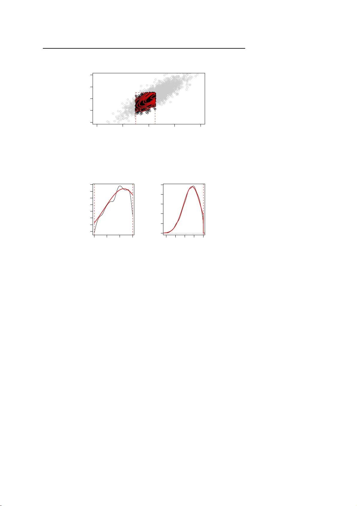
Noname manuscript No. (will be inserted by the editor) Moments Calculation For the Doubly T runcated Multivariate Normal Density Manjuna t h B G · Stefan W ilhelm This version: 23.06.2012 Abstract In the pr esent article we der ive an explicit expression for the trun- cated mean and variance for the multivariate normal distribution with ar- bitrary rectangular double truncation. W e use the moment generating ap- proach of T allis ( 1 961) a nd extend it to general µ , Σ and a ll combinations of truncation. As par t of the solution we also give a formula for the biva ri- ate marginal density of truncated multinormal variates. W e also pro ve an invariance property of some elements of the inver se covariance after trunca- tion. Computer a lgorithms for computing the truncated mean, variance and the bivariate marginal probabilities for doubly truncated multivariate normal variates have been written in R and are presented along with three examples. Keywords multivariate normal; double truncation; moment generating function; bivariate marginal density function; graphical models; conditional independence Mathema tics Subje ct Classifica tion (201 0) 60E05 · 6 2H05 B. G. Manjun ath CEAUL and DEIO, FCUL, University of Lisbon, Portugal E-mail: bgmanjunath @ gmail.com Stefan W ilhelm Department of Finance, Un iversity of Basel, Switzerland T el.: +49-172-3818512 E-mail: Stefan.W ilhelm@stud.unibas.ch 2 Manjunath B G, Stefan W ilhelm 1 Introducti on The multivaria te normal distribution arises frequently and has a wide ra nge of applications in fields like multivariate regression, B ayesian sta tistics or the analysis of Brownian motion. One motivation to deal with moments of the truncated multivariate normal distribution comes from the a nalysis of special financial derivative s (“auto-callables” or “ Expresszertifikate”) in Germa ny . These products c a n expire early depe nding on some restrictions of the un- derlying trajectory , if the underlying is above or below certain call levels. In the fra mework of Brownian motion the finite-dimensional distributions for log returns at any d points in time are multivaria te normal. When some of the multinormal variates X = ( x 1 , . . . , x d ) ′ ∼ N ( µ , Σ ) are subject to inequality constraints ( e.g. a i ≤ x i ≤ b i ), this results in truncated multivariate normal distributions. Several types of truncations and their moment calculation have bee n de - scribed so far , for example the one-sided rectangular truncation x ≥ a (T allis 1961), the ra ther unusual e lliptical and ra d ial truncations a ≤ x ′ R x ≤ b (T allis 1963) and the plane truncation C x ≥ p (T a llis 1965). Linear constraints like a ≤ C x ≤ b can often be reduced to rectangular truncation by transformation of the variables (in case of a full rank matrix C : a ∗ = C − 1 a ≤ x ≤ C − 1 b = b ∗ ), which makes the double rectangular truncation a ≤ x ≤ b especially important. The existing works on moment calculations differ in the number of vari- ables they consider (univaria te, bivaria te , multivariate) and the types of rect- angular truncation they allow ( single vs. double truncation). Single or one- sided truncation can be either from above ( x ≤ a ) or below ( x ≥ a ), but only on one side for a ll variables, whereas d ouble truncation a ≤ x ≤ b ca n have both lower and upper truncations points. Other distinguishin g features of previous works are further limitations or restrictions they impose on the type of d istribution (e.g. zero mean) and the methods they use to derive the results (e.g. direct integration or moment-generating function). Next, we will briefly outline the line of research. Rosenbaum ( 1961) gave an explicit formula for the moments of the biva ri- ate case with single truncation from below in both variables by direct inte- gration. His results for the bivariate normal distribution have been exte nde d by Shah and Parikh (1964), Regier and Hamdan (197 1) and Muth ´ en (19 9 0) to double truncation. For the multivariate case, T allis (196 1) derived an explicit e xpression for the first two moments in case of a singly truncated multivaria te normal den- sity with zero mea n vector a nd the correlation matrix R using the moment generating function. A memiya ( 1974) a nd Lee (19 7 9) extended the T allis (19 6 1) derivation to a ge ner al covariance matrix Σ and also ev a luated the relation- ship between the first two moments. Gupta and T ra cy ( 1976) and Lee (19 83) gave very simple recursive relationships between moments of any order f or the doubly truncated case. But since except for the mean there are f ewer equa- tions than p a rameters, these recurrent conditions do not uniquely identify Moments Calculation For th e Doubly T runcated Multivariate Normal Density 3 T able 1 S urvey of previous works on the momen t s for th e truncated m ultivariate normal distri- bution Author #V ariates T runcation F ocus Rosenbaum (1961) bivariate single moments for bivariate normal variates with single truncation, b 1 < y 1 < ∞ , b 2 < y 2 < ∞ T allis (1961) multivariate single moments for multivariate n ormal vari- ates with single truncation from below Shah and Parikh (1964) bivariate double recurrence relations between moment s Regier and Hamdan (1971) bivariate double an explicit formula only for the case of truncation from b e low at the same point in both variables Amemiya (1974) multivariate single relationship between first and second moments Gupta and T racy (1976) multivariate double recurrence relations between moment s Lee (1979) multivariate single recurr ence relations between moments Lee (1983) multivariate double recurrence relations between moment s Leppard and T allis (1989) multivariate single moments for multivariate n ormal distri- bution with single truncation Muth ´ en (1990) bivariate double moment s for b ivariate normal d istribu- tion with double truncation, b 1 < y 1 < a 1 , b 2 < y 2 < a 2 Manjunath/W ilhelm multivariate double moments for multivariate n ormal distri- bution with double truncation in all v ari- ables a ≤ x ≤ b moments of order ≥ 2 and are therefore not sufficient for the computation of the variance a nd other higher order moments. T able 1 summariz es our survey of existing publications dea ling with the computation of truncated moments and their limitations. Even though the rectangular truncation a ≤ x ≤ b can be found in many situations, no ex- plicit moment formulas for the truncated mean and variance in the general multivariate case of double truncation f rom below a nd/or above have been presented so far in the literature and are readily apparent. The contribution of this paper is to d erive these formulas for the first two truncated moments and to extend and generalize existing results on moment calculations from especially T allis (1 9 61); Lee (1983); Leppard and T a llis (1 9 89); Muth ´ en (1990). The remainder of this pape r is organized as f ollows. Section 2 presents the moment generating function (m.g.f ) for the doubly truncated multivariate normal case . In Sec tion 3 we d e rive the first and second moments by differen- tiating the m.g.f. These results are completed in Section 4 b y giving a f ormula for computing the bivaria te marginal density . In Section 5 we present two nu- merical exa mples and compare our results with simulation results. Section 6 links our results to the theory of gra phical models and derives some proper- ties of the inverse covariance matrix. Finally , Section 7 summarizes our results and gives a n outlook f or f ur ther research. 4 Manjunath B G, Stefan W ilhelm 2 Moment Genera ting Function The d –dimensional normal density with location pa r ameter v e ctor µ ∈ R d and non-sing ular covariance matrix Σ is given by ϕ µ , Σ ( x ) = 1 ( 2 π ) d /2 | Σ | 1/ 2 exp  − 1 2 ( x − µ ) ′ Σ − 1 ( x − µ )  , x ∈ R d . (1) The pertaining distribution function is denoted by Φ µ , Σ ( x ) . Correspondingly , the multivariate truncated normal density , truncated a t a and b , in R d , is de- fined as ϕ α µ , Σ ( x ) =    ϕ µ , Σ ( x ) P { a ≤ X ≤ b } , for a ≤ x ≤ b , 0, otherwise. (2) Denote α = P { a ≤ X ≤ b } as the f r action after truncation. The moment generating f unction (m.g.f) of a d –dimensional truncated random var iable X , truncated a t a and b , in R d , having the density f ( x ) is defined as the d – fold integral of the form m ( t ) = E  e t ′ X  = Z b a e t ′ x f ( x ) d x . Therefore, the m.g.f for the density in (2) is m ( t ) = 1 α ( 2 π ) d /2 | Σ | 1/ 2 Z b a exp  − 1 2 h ( x − µ ) ′ Σ − 1 ( x − µ ) − 2 t ′ x i  d x . (3 ) In the following, the moments are first derived for the special case µ = 0 . Later , the results will be generalized to all µ by applying a location transfor- mation. Now , consider only the exponent term in (3) for the ca se µ = 0 . Then we have − 1 2 h x ′ Σ − 1 x − 2 t ′ x i which can a lso be written a s 1 2 t ′ Σ t − 1 2 h ( x − ξ ) ′ Σ − 1 ( x − ξ ) i , where ξ = Σ t . Consequently , the m.g.f of the rectangularly doubly truncated multivari- ate normal is m ( t ) = e T α ( 2 π ) d /2 | Σ | 1/ 2 Z b a exp  − 1 2 h ( x − ξ ) ′ Σ − 1 ( x − ξ ) i  d x , (4) Moments Calculation For th e Doubly T runcated Multivariate Normal Density 5 where T = 1 2 t ′ Σ t . The a bove equation ca n be fur ther reduced to m ( t ) = e T α ( 2 π ) d /2 | Σ | 1/ 2 Z b − ξ a − ξ exp  − 1 2 x ′ Σ − 1 x  d x . (5) For notational convenience, we write equation (5) as m ( t ) = e T Φ α Σ (6) where Φ α Σ = 1 α ( 2 π ) d /2 | Σ | 1/ 2 Z b − ξ a − ξ exp  − 1 2 x ′ Σ − 1 x  d x . 3 First And Second Moment C a lculati on In this section we derive the first and second moments of the rectangularly doubly truncated multivariate normal density by differentiating the m.g.f. . Consequently , by taking the partial der ivative of ( 6) with respect to t i we have ∂ m ( t ) ∂ t i = e T ∂ Φ α Σ ∂ t i + Φ α Σ ∂ e T ∂ t i . (7) In the above equation the only essential terms which will be simplified are ∂ e T ∂ t i = e T d ∑ k = 1 σ i , k t k and ∂ Φ α Σ ∂ t i = ∂ ∂ t i Z b ∗ 1 a ∗ 1 ... Z b ∗ d a ∗ d ϕ α Σ ( x ) d x d ... d x 1 , (8) where a ∗ i = a i − ∑ d k = 1 σ i , k t k and b ∗ i = b i − ∑ d k = 1 σ i , k t k . Subsequently , (8 ) is ∂ Φ α Σ ∂ t i = d ∑ k = 1 σ i , k ( F k ( a ∗ k ) − F k ( b ∗ k ) ) , (9) where F i ( x ) = Z b ∗ 1 a ∗ 1 ... Z b ∗ i − 1 a ∗ i − 1 Z b ∗ i + 1 a ∗ i + 1 ... Z b ∗ d a ∗ d ϕ α Σ ( x 1 , .., x i − 1 , x , x i + 1 , .. x d ) d x d ... d x i + 1 d x i − 1 ... d x 1 . (10) 6 Manjunath B G, Stefan W ilhelm Note that at t k = 0, for a ll k = 1, 2 , ..., d , we have a ∗ i = a i and b ∗ i = b i . Therefore, F i ( x ) will be the i –th marginal density . An especially convenient way of computing these one-dimensional marginals is given in Ca rtinhour (1990). From (7) – (9) for k = 1, 2, ..., d all t k = 0. Hence, the first moment is E ( X i ) = ∂ m ( t ) ∂ t i | t = 0 = d ∑ k = 1 σ i , k ( F k ( a k ) − F k ( b k ) ) . (11) Now , by taking the partial derivative of (7) with respect to t j , we hav e ∂ 2 m ( t ) ∂ t j ∂ t i = e T ∂ 2 Φ α Σ ∂ t j ∂ t i + ∂ Φ α Σ ∂ t i ∂ e T ∂ t j + Φ α Σ ∂ 2 e T ∂ t j ∂ t i + ∂ e T ∂ t i ∂ Φ α Σ ∂ t j . (12) The essential terms for simplification are ∂ 2 e T ∂ t j ∂ t i = σ i , j and clearly , the partial derivative of (9) with respect to t j gives ∂ 2 Φ α Σ ∂ t j ∂ t i = d ∑ k = 1 σ i , k ∂ F k ( a ∗ k ) ∂ t j ! − d ∑ k = 1 σ i , k ∂ F k ( b ∗ k ) ∂ t j ! . (13) In the a bove equation merely consider the partial derivative of the marginal density F k ( a ∗ k ) with respect to t j . W ith f urther simplification it reduces to ∂ F k ( a ∗ k ) ∂ t j = ∂ ∂ t j Z b ∗ 1 a ∗ 1 ... Z b ∗ k − 1 a ∗ k − 1 Z b ∗ k + 1 a ∗ k + 1 ... Z b ∗ d a ∗ d ϕ α Σ ( x 1 , .., x k − 1 , a ∗ k , x k + 1 , .. x d ) d x − k = σ j , k a ∗ k F k ( a ∗ k ) σ k , k + ∑ q 6 = k  σ j , q − σ k , q σ j , k σ k , k   F k , q ( a ∗ k , a ∗ q ) − F k , q ( a ∗ k , b ∗ q )  , (14) where F k , q ( x , y ) = Z b ∗ 1 a ∗ 1 ... Z b ∗ k − 1 a ∗ k − 1 Z b ∗ k + 1 a ∗ k + 1 ... Z b ∗ q − 1 a ∗ q − 1 Z b ∗ q + 1 a ∗ q + 1 ... Z b ∗ d a ∗ d ϕ α Σ ( x , y , x − k , − q ) d x − k , − q , (15) and the short form x − k denotes the vector ( x 1 , .., x k − 1 , x k + 1 , .. x d ) ′ in ( d − 1 ) – dimensions and x − k , − q denotes the ( d − 2 ) – dimensional vector ( x 1 , ..., x k − 1 , x k + 1 , ..., x q − 1 , x q + 1 , ..., x d ) ′ for k 6 = q . The above equation (14) is deduced f rom Lee (197 9 ), pp. 1 67. Note that for all t k = 0 the term F k , q ( x , y ) will be the bi- variate marginal density for which we will give a f ormula in the next section. Moments Calculation For th e Doubly T runcated Multivariate Normal Density 7 Subsequently , ∂ F k ( b ∗ k ) ∂ t j can be obta ined by substituting a ∗ k by b ∗ k . From (12) – (15) at a ll t k = 0, k = 1, 2, . .., d , the second moment is E ( X i X j ) = ∂ 2 m ( t ) ∂ t j ∂ t i | t = 0 = σ i , j + d ∑ k = 1 σ i , k σ j , k ( a k F k ( a k ) − b k F k ( b k ) ) σ k , k + d ∑ k = 1 σ i , k ∑ q 6 = k  σ j , q − σ k , q σ j , k σ k , k  h F k , q ( a k , a q ) − F k , q ( a k , b q )  −  F k , q ( b k , a q ) − F k , q ( b k , b q ) i . (16) Having derived expressions f or the first and second moments for double truncation in ca se of µ = 0 , we will now genera lize to all µ : if Y ∼ N ( µ , Σ ) with a ∗ ≤ y ≤ b ∗ , then X = Y − µ ∼ N ( 0 , Σ ) with a = a ∗ − µ ≤ x ≤ b ∗ − µ = b and E ( Y ) = E ( X ) + µ and C o v ( Y ) = Co v ( X ) . Equations (11) and (1 6) can then be used to c ompute E ( X ) a nd C o v ( X ) . Hence, for general µ , the first moment is E ( Y i ) = d ∑ k = 1 σ i , k ( F k ( a k ) − F k ( b k ) ) + µ i . (17) The covariance matrix C o v ( Y i , Y j ) = C ov ( X i , X j ) = E ( X i X j ) − E ( X i ) E ( X j ) (18) is invariant to the shift in location. The equations (17) and (18) in combination with (11) and (16) form our desired result and allow the calculation of the truncated mea n and truncated variance for general double truncation. A formula f or the term F k , q ( x k , x q ) , the bivariate marginal density , will be given in the next section. W e ha ve implemented the moment calculation for mean vector mea n , covari- ance matrix sigma and truncation vectors lower and upper as a function mtmvno rm(me an, sig ma, lower, upper) in the R packa ge tmv tnorm (W ilhelm a nd Manjunath 20 10a; ? ), where the code is open source. In Section 5 we show a usage example for this function. 4 Bivariat e Marginal Density Computati on In order to compute the bivariate marginal density in this section we ma inly follow T allis ( 1961), p. 223 and Leppard and T a llis (19 89 ) who implicitly used the biva riate marginal density as pa rt of the moments calcula tion for single truncation, eva luated at the integration bounds. However , we extend it to the 8 Manjunath B G, Stefan W ilhelm doubly truncated case and state the function for all points within the support region. W ithout loss of genera lity we use a z-transformation for a ll variates x = ( x 1 , . . . , x d ) ′ as well as f or all lower and upper truncation points a = ( a 1 , . . . , a d ) ′ and b = ( b 1 , . . . , b d ) ′ , resulting in a N ( 0, R ) distribution with correlation ma - trix R for the standardized untruncated va riates. In this section we treat all variables as if they are z-transformed, lea ving the notation unchanged. For computing the bivaria te marginal density F q , r ( x q , x r ) with a q ≤ x q ≤ b q , a r ≤ x r ≤ b r , q 6 = r , we use the fact that f or truncated normal densities the conditional densities are truncated normal aga in. The following relationship holds f or x s , z s ∈ R d − 2 if we condition on x q = c q and x r = c r ( s 6 = q 6 = r ) : α − 1 ϕ d ( x s , x q = c q , x r = c r ; R ) = α − 1 ϕ ( c q , c r ; ρ qr ) ϕ d − 2 ( z s ; R qr ) , (19) where z s = ( x s − β s q . r c q − β sr . q c r ) / q ( 1 − ρ 2 s q ) ( 1 − ρ 2 sr . q ) (20) and R qr is the matrix of sec ond-order partial correlation coefficients for s 6 = q 6 = r . β s q . r and β sr . q are the pa r tial regressio n coefficients of x s on x q and x r respectively and ρ sr . q is the partial correlation coefficient between x s and x r for fixed x q . Integrating out ( d − 2 ) variables x s leads to F q , r ( x q , x r ) as a product of a bivari- ate normal d e nsity ϕ ( x q , x r ) and a ( d − 2 ) -dimension normal integral Φ d − 2 : F q , r ( x q = c q , x r = c r ) = Z b 1 a 1 ... Z b q − 1 a q − 1 Z b q + 1 a q + 1 ... Z b r − 1 a r − 1 Z b r + 1 a r + 1 ... Z b d a d ϕ α R ( x s , c q , c r ) d x s = α − 1 ϕ ( c q , c r ; ρ qr ) Φ d − 2 ( A q r s ; B q r s ; R qr ) (2 1) where A q r s and B q r s denote the lower and uppe r integra tion bounds of Φ d − 2 given x q = c q and x r = c r : A q r s = ( a s − β s q . r c q − β sr . q c r ) / q ( 1 − ρ 2 s q ) ( 1 − ρ 2 sr . q ) (22) B q r s = ( b s − β s q . r c q − β sr . q c r ) / q ( 1 − ρ 2 s q ) ( 1 − ρ 2 sr . q ) . (23) The computation of F q , r ( x q , x r ) just needs the evaluation of the normal inte- gral Φ d − 2 in d − 2 dimensions, which is readily a vailable in most statistics software packages, for exa mple as the function pm vnorm( ) in the R pac ka ge mvtnor m ( ? ). The biva riate marginal density function dtmvno rm(x, mean, sigma, lower, upper, margin=c (q,r)) is also par t of the R package tmv tnorm (W ilhelm and Manjunath 2010 a; ? ), where read ers c a n find the source code a s well as help files and additional examples. Moments Calculation For th e Doubly T runcated Multivariate Normal Density 9 −4 −2 0 2 4 −4 −2 0 2 4 bivariate marginal density (x 1 ,x 2 ) x 1 x 2 0.05 0.05 0.1 0.15 0.15 0.25 0.3 0.4 0.45 Fig. 1 Contour plot for the bivariate truncated density function −1.0 −0.5 0.0 0.5 0.2 0.4 0.6 0.8 Marginal density x 1 x 1 Density −3 −2 −1 0 1 0.0 0.1 0.2 0.3 0.4 0.5 Marginal density x 2 x 2 Density Fig. 2 Marginal densities F k ( x ) ( k = 1, 2) for x 1 and x 2 obtained from Kernel density estimat ion of random samples and from direct evaluation of F k ( x ) 5 Numerica l Exa mples 5.1 Example 1 W e will use the following bivaria te e xample with µ = ( 0.5, 0 .5 ) ′ and covari- ance matrix Σ Σ =  1 1.2 1.2 2  as well a s lower and upper truncation points a = ( − 1, − ∞ ) ′ , b = ( 0 . 5, 1 ) ′ , i.e. x 1 is doubly , while x 2 is singly trun cate d . The bivaria te marginal den- sity F q , r ( x , y ) is the density f unction itself a nd is shown in figure 1, the one- dimensional densities F k ( x ) ( k = 1, 2) in figure 2. The moment ca lcula tion f or our example can be performed in R as 10 Manjunath B G, Stefan W ilhelm 0 2000 6000 10000 −0.20 −0.18 −0.16 −0.14 −0.12 −0.10 Monte Carlo estimator for µ ^ 1 sample size µ ^ 1 theoretical value 95% MC confidence interval 0 2000 6000 10000 −0.50 −0.45 −0.40 −0.35 −0.30 Monte Carlo estimator for µ ^ 2 sample size µ ^ 2 theoretical value 95% MC confidence interval Fig. 3 T race plots of th e Mont e Carlo estimator for µ ∗ > librar y(tmvt norm) > mu <- c(0.5, 0.5) > sigma <- matrix( c(1, 1 .2, 1.2, 2), 2, 2) > a <- c(-1, -Inf) > b <- c(0.5, 1) > moment s <- mtmvnor m(mean =mu, sigm a=sigm a, > lower= a, u pper= b) and results in µ ∗ = ( − 0. 152, − 0.3 88 ) ′ and covariance ma trix Σ ∗ =  0.163 0.1 61 0.161 0.6 06  The tra ce plots in figures 3 and 4 show the evolution of a Monte Carlo esti- mate for the elements of the mean v e ctor and the covariance matrix respec- tively for growing sample sizes. Furthermore, the 95% c onfidence interva l obtained f rom Monte Carlo using the f ull sample of 100 00 items is shown. All confidence interva ls contain the true theoretical va lue, but Monte Ca rlo esti- mates still show substantial variation ev e n with a sa mple size of 1 0000. Sim- ulation from a truncated multivariate d istribution and calculating the sample mean or the sa mple covariance respectively also lea ds to consistent estimates of µ ∗ and Σ ∗ . S ince the ra te of convergence of the MC estimator is O ( √ n ) , one has to ensure sufficient Monte C a rlo iterations in order to have a good approximation or to choose variance reduction techniques. Moments Calculation For th e Doubly T runcated Multivariate Normal Density 11 0 2000 6000 10000 0.10 0.12 0.14 0.16 0.18 Monte Carlo estimator for Cov ( x 1 , x 1 ) sample size Cov ( x 1 , x 1 ) theoretical value 0 2000 6000 10000 0.10 0.12 0.14 0.16 0.18 0.20 Monte Carlo estimator for Cov ( x 1 , x 2 ) sample size Cov ( x 1 , x 2 ) theoretical value 0 2000 6000 10000 0.4 0.5 0.6 0.7 0.8 Monte Carlo estimator for Cov ( x 2 , x 2 ) sample size Cov ( x 2 , x 2 ) theoretical value Fig. 4 T race plots of th e Mont e Carlo estimator for t he 3 elements of Σ ∗ ( σ ∗ 11 , σ ∗ 12 = σ ∗ 21 and σ ∗ 22 ) 5.2 Example 2 Let µ = ( 0 , 0, 0 ) ′ ,the cova riance matrix Σ =   1.1 1.2 0 1.2 2 − 0.8 0 − 0.8 3   and the lower and upper trun cation points a = ( − 1, − ∞ , − ∞ ) ′ and b = ( 0. 5, ∞ , ∞ ) ′ , then the only truncated va riable is x 1 , which is fur ther more un- correlated with x 3 . Our formula results in µ ∗ = c ( − 0.2 10, − 0.2 29, 0 ) ′ and Σ ∗ =   0.174 0.1 90 0.0 0.190 0.8 98 − 0. 8 0 − 0. 8 3.0   For this specia l case of only k < d tr uncated va riables ( x 1 , . . . , x k ) , the remain- ing d − k var iables ( x k + 1 , . . . , x d ) can be regressed on the truncated variables, and a simple formula for the mea n and covariance matrix can be given (see Johnson and Kotz (1 9 71), p. 70). Let the cova riance matrix Σ of ( x 1 , . . . , x d ) be partitioned as Σ =  V 11 V 12 V 21 V 22  (24) 12 Manjunath B G, Stefan W ilhelm where V 11 denotes the k × k cova riance matrix of ( x 1 , . . . , x k ) . The mean vec- tor 1 and the cova riance matrix Σ ∗ of all d va riables can be computed as ( ξ ′ 1 , ξ ′ 1 V − 1 11 V 12 ) (25) and Σ ∗ =  U 11 U 11 V − 1 11 V 12 V 21 V − 1 11 U 11 V 22 − V 21 ( V − 1 11 − V − 1 11 U 11 V − 1 11 ) V 12  (26) where ξ ′ 1 and U 11 are the mean and cova riance of the ( x 1 , . . . , x k ) af ter trun- cation. The mean a nd standard deviation for the univariate truncated normal x 1 are ξ 1 = µ ∗ 1 = σ 11 ϕ µ 1 , σ 11 ( a 1 ) − ϕ µ 1 , σ 11 ( b 1 ) Φ µ 1 , σ 11 ( b 1 ) − Φ µ 1 , σ 11 ( a 1 ) σ ∗ 11 = σ 11 + σ 11 a 1 ϕ µ 1 , σ 11 ( a 1 ) − b 1 ϕ µ 1 , σ 11 ( b 1 ) Φ µ 1 , σ 11 ( b 1 ) − Φ µ 1 , σ 11 ( a 1 ) Letting U 11 = σ ∗ 11 and inserting ξ 1 and U 11 into e quations (25) and (26), one can verify our f ormula and the results for µ ∗ and Σ ∗ . However , the crux in using the Johnson/Kotz formula is the need to first compute the moments of the truncated variables ( x 1 , . . . , x k ) for k ≥ 2. But this has been e x actly the subject of our p a per . 6 Moment Calcu lation and Conditiona l Indepe ndence In this section we establish a link between our moment c alculation and the theory of graphical models (Whittaker (1 990), Edwards (199 5) a nd Lauritzen (1996)). W e present some properties of the inverse covariance matr ix and show how the depe ndence structure of va riables is a ffec te d a fter selection. Graphical modelling uses graphical representations of va riables as nodes in a graph and d e pendencies among them as edges. A key concept in graphi- cal modelling is the conditional independe nce property . T wo variables X and Y are conditional independent given a va riable or a set of variables Z (nota- tion X ⊥ ⊥ Y | Z ), when X and Y are independent af te r pa rtialling out the effect of Z . For conditional independent X and Y the edge between them in the graph is omitted a nd the joint density factorizes as f ( x , y | z ) = f ( x | z ) f ( y | z ) . Conditional independence is equivalent to hav ing zero elements Ω x y in the inverse covariance ma trix Ω = Σ − 1 as well as having a zero pa rtial co- variance/correlation between X and Y given the remaining variables: X ⊥ ⊥ Y | Rest ⇐ ⇒ Ω x y = 0 ⇐ ⇒ ρ x y . Re s t = 0 1 The formula for the truncated mean given in Johnson and Kotz (1971), p. 70 is only valid for a zero-mean vector or after dem eaning all v ariables appropriately . For non-zero m eans µ = ( µ 1 , µ 2 ) ′ it will be ( ξ ′ 1 , µ 2 + ( ξ ′ 1 − µ 1 ) V − 1 11 V 12 ) . Moments Calculation For th e Doubly T runcated Multivariate Normal Density 13 Both marginal independe nce a nd conditional independence b e tween va ri- ables simplify the computations of the truncated covariance in equation (16). In the presence of conditional independence of i a nd j given q , the terms σ i j − σ i q σ − 1 qq σ q j = 0 vanish as they reflect the partial covariance of i and j given q . As has been shown by Marchetti and Sta nghellini (2008), the conditional independence property is preserved a fter selection, i.e. the inverse covariance matrices Ω a nd Ω ∗ before a nd after truncation share the same zero-elements. W e prove that ma ny elements of the precision matrix are invariant to trun- cation. For the ca se of k < d truncated va r iables, we define the set of trun- cated va riables with T = { x 1 , . . . , x k } , and the remaining d − k v a riables as S = { x k + 1 , . . . , x d } . W e c a n show that the off-diagonal e lements Ω i , j are in- variant after truncation for i ∈ T ∪ S a nd j ∈ S : Proposition 6.1. The off-diagonal elements Ω i , j and the diagonal elements Ω j , j are invariant after truncation for i ∈ T ∪ S and j ∈ S . Proof. The proof is a direct applica tion of the Johnson/Kotz formula in equa- tion (2 6) in the previous section. A s a result of the formula for partitioned inverse matrices (Greene (2 003), section A . 5.3), the c orresponding inverse co- variance matrix Ω of the partitioned covariance matrix Σ is Ω =  V − 1 11 ( I + V 12 F 2 V 21 V − 1 11 ) − V − 1 11 V 12 F 2 − F 2 V 21 V − 1 11 F 2  (27) with F 2 = ( V 22 − V 21 V − 1 11 V 12 ) − 1 . Inverting the truncated covariance matrix Σ ∗ in e quation (2 6) using the formula for the pa rtitioned inverse leads to the truncated precision ma trix Ω ∗ =  U − 1 11 + V − 1 11 V 12 F 2 V 21 V − 1 11 − V − 1 11 V 12 F 2 − F 2 V 21 V − 1 11 F 2  (28) where the Ω ∗ 12 and Ω ∗ 21 elements are the same as Ω 12 and Ω 21 respectively . The same is true for the elements in Ω ∗ 22 , especially the diagonal elements in Ω ∗ 22 . Here, we prove this invariance property only for a subset of truncated variables. Based on our experiments we conjecture that the same is true also for the case of full truncation ( i.e. all off-diagonal elements in Ω ∗ 11 ), but we do not give a rigorous proof here and leave it to future research. 6.1 Example 3 W e illustrate the invariance of the elements of the inverse covariance matrix with the fa mous mathematics marks example used in Whittaker (199 0) and Edwards (1995), p. 49. The independence graph of the five variables ( W , V , X , 14 Manjunath B G, Stefan W ilhelm Y , Z ) in this exa mple takes the form of a butterfly . mechanics (V) vectors (W) algebra (X) analysis (Y) statistics (Z) Here, we have the conditional independencies ( W , V ) ⊥ ⊥ ( Y , Z ) | X . A corresponding precision matrix might look like (sample da ta; zero-elements marked as ” . ”): Ω =       1 0.2 0.3 . . 0.2 1 − 0.1 . . 0.3 − 0.1 1 0.4 0.5 . . 0.4 1 0. 2 . . 0.5 0.2 1       (29) After truncation in some varia b le s (f or example ( W , V , X ) as − 2 ≤ W ≤ 1, − 1 ≤ V ≤ 1 , 0 ≤ X ≤ 1), we apply equation (16) to compute the truncated second moment and the inverse covaria nce matrix as: Ω ∗ =       1.88 0. 2 0.3 . . 0.2 3.4 5 − 0.1 . . 0.3 − 0 .1 12.6 7 0.4 0.5 . . 0.4 1 0. 2 . . 0.5 0.2 1       (30) The precision matr ix Ω ∗ after selection differs from Ω only in the d iagonal elements of ( W , V , X ) . From Ω ∗ we can read how pa rtial correlations between variables have changed due to the selection process. Each d iagonal element Ω y y of the precision matrix is the inverse of the partial variance af ter regressing on all other variables (Whittaker (1 990),p. 1 43). Since only those diagonal elements in the precision ma tr ix for the k ≤ d of the truncated variables will change a fter selection, this lea ds to the idea to just compute these k elements after selection rather than the full k ( k + 1 ) / 2 sym- metric elements in the truncated covariance matrix a nd applying the J ohn- son/Kotz f ormula for the remaining d − k variables. However , the inverse partial variance of a scalar Y given the remaining variables X = { x 1 , . . . , x d } \ y Ω ∗ y y = h Σ ∗ y . X i − 1 = h Σ ∗ y y − Σ ∗ y X Σ ∗ − 1 X X Σ ∗ X y i − 1 still requires the truncated covariance results der ive d in Section 3. Moments Calculation For th e Doubly T runcated Multivariate Normal Density 15 7 Summa ry In this pa per we derived a f ormula for the first and second moments of the doubly truncated multivariate normal distribution a nd for their b iva ri- ate marginal de nsity . A n implementation for both formulas has been made available in the R statistics software a s pa rt of the tmvtn orm package. W e linked our results to the theory of graphical models and proved an invari- ance property for elements of the precision matrix. Further research can dea l with other types of truncation than we considered (e. g. elliptical). Another line of research can look at the moments of the d oubly truncated multivari- ate Stud e nt-t distribution, which contains the truncated multivariate normal distribution as a special ca se. References Amemiya T (1974) Multivariate regression an d simultaneous equations models when the depen- dent variables are truncated normal. Econometrica 42:999–1012 Cartinhour J (1990) One -d imensional marginal density functions of a truncated multivariate nor- mal density function. Communications in St atistics - Theory and Meth od s 19:197–203 Edwards D (1995) Introduction t o graphical modelling. Springer Genz A, B retz F , Miwa T , Mi X, Leisch F , Scheipl F , Hothorn T (2010) mvtn orm: Multivariate nor- mal and t distributions. URL http://CRAN .R- pro ject.org/package=mvtnorm , R package version 0.9-95 Greene WH (2003) Econometric Analysis, 5th ed n. Prentice-Hal l Gupta AK, T racy DS (1976) Recurrence relations for the mome n ts of truncated m ultinormal dis- tribution. Communications in Statistics - Th eory and Methods 5(9):855–865 Johnson NL, Kotz S (1971) Distributions in Statistics: Continuous Multivariate Distributions. John W iley & Sons Lauritzen S (1996) Graphical Mode ls. Oxfor d University Press Lee LF (1979) On the first and second moments of the truncated multi-normal distribution and a simple estimator . Economics Letters 3:165–169 Lee LF (1983) The determ ination of m oments of t he doubly truncated multivariate tobit model. Economics Letters 11:245–250 Leppard P , T allis GM (1989) Algorithm AS 249: Evaluation of the m e an and covarianc e of the truncated multinormal distribution. Applied Statistics 38:543–553 Marchetti GM, Stanghellini E (2008) A note on d istortions induced by truncation with applica- tions to linear regression syste ms. St atistics & Probability Letters 78:824829 Muth ´ en B (1990) Moment s of t he cen sored and truncated bivariate normal distribution. British Journal of Mathematical and St atistical Psychology 43:131–143 Regier MH, Hamdan MA (1971) Correlation in a b ivariate normal distribution with truncation in both variables. Australian Journal of S t atistics 13:77–82 Rosenbaum S (1961) Moments of a truncated b ivariate normal distribution. Journal of th e Royal Statistical Society Series B (Meth odological) 23:405–408 Shah SM, Parikh NT (1964) Mome nts of single and doubly truncated stan d ard bivariate n ormal distribution. V idya (Gujarat University) 7:82–91 T allis GM (1961) The moment ge nerating function of the truncated multinormal d istribution. Journal of the Royal Statistical Society , Series B (Methodological) 23(1):223–229 T allis GM (1963) Elliptical and radial truncation in normal populations. The Annals of Mathe - matical Statistics 34(3):940–944 T allis GM (1965) Plane truncation in normal populations. Journal of the Royal Statistical Society , Series B (Methodological) 27(2):301–307 Whittaker J (1990) Graphical models in applied multivariate statistics. John W iley & Sons 16 Manjunath B G, Stefan W ilhelm W ilhelm S, Manjunath BG (2010a) tmvtnorm: A Package for the T run- cated Mul tivariate Normal Distribution. The R Journal 2(1):25–29, URL http://j ournal.r- project.org/archive/2010- 1/RJournal_2010- 1_Wilhelm+Manjunath.pdf W ilhelm S, Manjun ath BG (2010b) tmv tnorm: T runcated multivariate normal distribution and Student t distribution. URL http://CRA N.R- project.org/package=tmvtnorm , R package version 1.1-5