Total Variation and Eulers Elastica for Supervised Learning

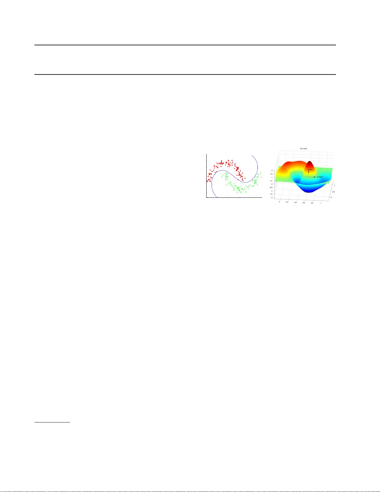
T otal V ariation and Euler’s Elastica for Sup ervised Learning T ong Lin tonglin123@gmail.com Hanlin Xue xuehl@cis.pku.edu.cn Ling W ang* ling.w ang.nj@gmail.com Hongbin Zha zha@cis.pku.edu.cn The Key Lab oratory of Mac hine P erception (Ministry of Education), P eking Univ ersit y , Beijing, China *L TCI, T´ el ´ ecom ParisT ec h, P aris, F rance Abstract In recen t y ears, total v ariation (TV) and Eu- ler’s elastica (EE) hav e b een successfully ap- plied to image pro cessing tasks such as de- noising and inpain ting. This pap er inv es- tigates ho w to extend TV and EE to the sup ervised learning settings on high dimen- sional data. The sup ervised learning problem can b e form ulated as an energy functional minimization under Tikhono v regularization sc heme, where the energy is comp osed of a squared loss and a total v ariation smo oth- ing (or Euler’s elastica smo othing). Its so- lution via v ariational principles leads to an Euler-Lagrange PDE. How ever, the PDE is alw ays high-dimensional and cannot b e di- rectly solved b y common metho ds. Instead, radial basis functions are utilized to approxi- mate the target function, reducing the prob- lem to finding the linear co efficients of basis functions. W e apply the prop osed metho ds to supervised learning tasks (including binary classification, m ulti-class classification, and regression) on b enchmark data sets. Exten- siv e experiments hav e demonstrated promis- ing results of the prop osed metho ds. 1. In tro duction Sup ervised learning ( Bishop , 2006 ; Hastie T. , 2009 ) in- fers a function that maps inputs to desired outputs under the guidance of training data. Two main tasks in sup ervised learning are classification and regres- sion. A h uge num b er of sup ervised learning methods ha v e b een developed in several decades (see a com- App earing in Pr o c ee dings of the 29 th International Confer- enc e on Machine L e arning , Edin burgh, Scotland, UK, 2012. Cop yrigh t 2012 b y the author(s)/owner(s). 0 0.2 0.4 0.6 0.8 1 0 0.2 0.4 0.6 0.8 1 Euler Elastica decision boundary Figure 1. Results on tw o mo on data b y the EE classifier: (Left) decision boundary; (Righ t) learned target function. prehensiv e empirical comparison of these metho ds in ( Caruana & Niculescu-Mizil , 2006 )). Existing meth- o ds can b e roughly divided into statistics based and function learning based ( Kotsian tis et al. , 2006 ). One adv an tage of function learning metho ds is that p ow- erful mathematical theories in functional analysis can b e utilized rather than doing optimizations on discrete data p oin ts. Most function learning metho ds can b e derived from Tikhono v regularization, which minimizes a loss term plus a smo othing regularizer. The most successful classification and regression metho d is SVM ( Bishop , 2006 ; Hastie T. , 2009 ; Sha we-T a ylor & Cristianini , 2000 ), whose cost function is comp osed of a hinge loss and a RKHS norm determined by a k ernel. Re- placing the hinge loss b y a squared loss, the mo dified algorithm is called Regularized Least Squares (RLS) metho d ( Rifkin , 2002 ). In addition, manifold regu- larization ( Belkin et al. , 2006 ) introduced a regular- izer of squared gradien t magnitude on manifolds. Its discrete version amoun ts to graph Laplacian regular- ization ( Nadler et al. , 2009 ; Zhou & Sch¨ olk opf , 2005 ), whic h approximates the original energy functional. A most recent w ork is the geometric lev el set (GLS) classifier ( V arshney & Willsky , 2010 ), with an energy functional comp osed of a margin-based loss and a ge- ometric regularization term based on the surface area T otal V ariation and Euler’s Elastica for Sup ervised Learning of the decision b oundary . Experiments show ed that GLS is comp etitive with SVM and other state-of-the- art classifiers. In this paper, the supervised learning problem is for- m ulated as an energy functional minimization un- der Tikhonov regularization sc heme, with the en- ergy comp osed of a squared loss and a total v aria- tion (TV) penalty or an Euler’s elastica (EE) p enalty . Since the TV and EE mo dels hav e achiev ed great success in image denoising and image inpainting ( Aub ert & Kornprobst , 2006 ; Barb ero & Sra , 2011 ; Chan & Shen , 2005 ), a natural question is whether the success of TV and EE mo dels on image pro cessing ap- plications can b e transferred to high dimensional data analysis such as sup ervised learning. This paper in ves- tigates the question b y extending TV and EE models to sup ervised learning settings, and ev aluating their p erformance on b enchmark data sets against state-of- the-art metho ds. Figure 1 shows the classification re- sult on the p opular tw o mo on data by the EE clas- sifier, and the learned target function. Interestingly , the GLS classifier ( V arshney & Willsky , 2010 ) is also motiv ated by image processing techniques, and its gra- dien t descent time marching leads to a mean curv ature flo w. The pap er is organized as follows. W e b egin with a brief review of TV and EE in Section 2. In Section 3 the prop osed mo dels are describ ed, and n umerical solutions are developed in Section 4. Section 5 presents the experimental results, and Section 6 concludes this pap er. 2. Preliminaries W e briefly in tro duce total v ariation and Euler’s elas- tica from an image pro cessing p ersp ective, and p oint out connections with prior w ork in the mac hine learn- ing literature. 2.1. T otal V ariation (TV) The total v ariation of a 1D real-v alued function f is defined as V a b ( f ) = sup n p − 1 ∑ i =0 | f ( x i +1 ) − f ( x i ) | , where the supremum runs ov er all partitions of giv en in terv al [ a, b ]. If f is differentiable, the total v ariation can b e written as V a b ( f ) = ∫ b a | f ′ ( x ) | dx. Simply , it is a measure of the total quantit y of the c hange of a function. Notice that if f ′ ( x ) > 0 , x ∈ [ a, b ], it is exactly f ( b ) − f ( a ) b y the basic theorem of calculus. T otal v ariation has b een widely used for im- age pro cessing tasks such as denoising and inpainting. The pioneering w ork is Rudin, Osher, and F atemi’s image denoising mo del ( Rudin et al. , 1992 ): J = ∫ Ω (( I − I 0 ) 2 + λ |∇ I | ) dx, where I 0 is the input image with noise, I the desired output image, λ a regulation parameter that balances t w o terms, and Ω a 2 D image domain. The first fitting term measures the fidelity to the input, while the sec- ond is a p -Sob olev regularization term ( p = 1) where ∇ I is understo o d in the distributional sense. The main merit is to preserve significant image edges during denoising ( Aub ert & Kornprobst , 2006 ; Chan & Shen , 2005 ). Note that TV ma y ha ve different definitions ( Barb ero & Sra , 2011 ). In the mac hine learning literature, p -Sobolev regular- izer can be found in nonparametric smo othing splines, generalized additive mo dels, and pro jection pursuit re- gression mo dels ( Hastie T. , 2009 ). Sp ecifically , Belkin et al. prop osed the manifold regularization term ∫ x ∈ M |∇ M f | 2 dx, on a manifold M ( Belkin et al. , 2006 ). On the other hand, discrete graph Laplacian regularization w as dis- cussed in ( Zhou & Sc h¨ olkopf , 2005 ) as ∑ v ∈ V |∇ v f | p , where v is a v ertex from V , and p is an arbitrary num- b er. This p enalty measures the roughness of f ov er a graph. 2.2. Euler’s Elastica (EE) Euler (1744) first introduced the elastica energy for a curve on mo deling torsion-free elastic ro ds. Then Mumford ( Mumford , 1991 ) rein tro duced elastica in to computer vision. Later, elastica based image inpaint- ing metho ds were developed in ( Chan et al. , 2002 ; Masnou & Morel , 1998 ). A curve γ is said to be Euler’s elastica if it is the equilibrium curv e of the elasticit y energy: E [ γ ] = ∫ γ ( a + bκ 2 ) ds, (1) where a and b stand for t wo positive constan t weigh ts, κ denotes the scalar curv ature, and ds is the arc length T otal V ariation and Euler’s Elastica for Sup ervised Learning elemen t. Euler obtained the energy in studying the steady shape of a thin and torsion-free ro d under ex- ternal forces. The curv e implies the lo west elastica en- ergy , thus getting its name. According to ( Mumford , 1991 ), the key link b et w een the elastica and image inpain ting relies on the the interpolation capabilit y of elastica. That is, elastica can comply to the con- nectivit y principle b etter than total v ariation. Suc h kinds of ”nonlinear splines”, like classical p olynomial splines, are natural to ols for completing the missing or o ccluded edges. The Euler’s elastica based inpain ting mo del w as pro- p osed as ( Chan & Shen , 2005 ) J = ∫ Ω \ D ( I − I 0 ) 2 dx + λ ∫ Ω ( a + bκ 2 ) |∇ I | dx, (2) where D is the region to b e inpainted, Ω the whole image domain, and κ the curv ature of the associated lev el set curv e with κ = ∇ · ( ∇ I |∇ I | ) . (3) By using calculus of v ariation, its minimization is re- duced to an nonlinear Euler-Lagrange equation. The finite difference scheme can b e used to giv e numerical implemen tation, and experimental results sho w that the EE based inpainting p erforms better than its TV v ersion. Elastica can b e regarded as an extension of total v ari- ation, since elastica degenerates to total v ariation if set a = 1 and b = 0. In fact, elastica is a combination of total v ariation suppressing oscillations in the gradi- en t direction, and a curv ature regularization term that p enalizes non-smo oth lev el set curv es (see Figure 1 ). 3. The Prop osed F ramew ork 3.1. Problem Setup The general sup ervised learning problem can b e describ ed as follo ws: giv en a training data { ( x 1 , y 1 ) , ... ( x n , y n ) } with data p oints x i ∈ Ω ⊂ R d and corresp onding target v aribles y i , the goal is to estimate an unknown function u ( x ) for a new p oint x . The difference b etw een classification and regres- sion lies only in the corresponding target v alues, with one discrete and the other contin uous. The widely used Tikhonov regularization framework for super- vised learning can b e form ulated as: min n ∑ i =1 L ( u ( x i ) , y i ) + λS ( u ) , (4) where L denotes a loss function and S ( u ) is a smo oth- ing term. A v ariet y of loss functions L ha ve b een pro- p osed in the literature: hinge loss for SVM, squared loss for RLS, logistic loss for logistic regression, Huber loss, exponential loss, and among others. Throughout the pap er, squared loss is used in all mo dels due to its rather simpler differen tial form. 3.2. Laplacian Regularization (LR) A commonly used mo del using squared loss can be written as min n ∑ i =1 ( u ( x i ) − y i ) 2 + λS ( u ) . (5) If the RKHS norm is used for the smo othing term, the mo del is called regularized least squares (RLS) ( Rifkin , 2002 ). Another natural choice is the squared L 2 -norm of the gradien t: S ( u ) = |∇ u | 2 , as proposed in ( Belkin et al. , 2006 ). Under a con tinuous setting, we get the follo wing Laplacian regularization (LR) model: J LR [ u ] = ∫ Ω (( u − y ) 2 + λ |∇ u | 2 ) d x . (6) This LR mo del has b een widely used in the image pro- cessing literatures. Using calculus of v ariations, the minimization can b e reduced to the following Euler- Lagrange partial differential equation (PDE) with a natural b oundary condition along ∂ Ω: { − λ △ u + ( u − y ) = 0 ∂ u ∂ n | ∂ Ω = 0 , (7) where △ u is the Laplacian of u , and n denotes the nor- mal v ector along the boundary ∂ Ω. This PDE is rela- tiv ely simple and can b e solved using common metho ds in t w o and three dimensions. The next Section pro- vides a function appro ximation metho d for solving the PDE in high dimensions. 3.3. T otal V ariation (TV) based Smo othing Our goal is to explore how TV and EE can b e ap- plied to classification and regression problems on high dimensional data sets. A t ypical pro cedure has three steps: (a) Set the function learning problem under a con tin uous setting and design a prop er energy func- tional; (b) Deriv e the Euler-Lagrange PDE via the cal- culus of v ariations; (c) Solve the PDE on discrete data p oin ts. Similar to image denoising, total v ariation (TV) based sup ervised learning can b e form ulated as J T V [ u ] = ∫ Ω ( u − y ) 2 d x + λ ∫ Ω |∇ u | d x . (8) Note that for binary classification the zero level set of u serv es as the final decision b oundary . The only T otal V ariation and Euler’s Elastica for Sup ervised Learning difference b etw een LR and TV is just the p -Sob olev regularizer with p = 2 for LR and p = 1 for TV. In- tuitiv ely , LR p enalizes to o muc h gradients on edges, while TV can p ermit sharp er edges near the decision b oundaries b et w een tw o classes. 3.4. Euler’s Elastica (EE) based Smo othing Elastica based supervised learning can be formulated as J E E [ u ] = ∫ Ω ( u − y ) 2 d x + λ ∫ Ω ( a + bκ 2 ) |∇ u | d x , (9) where κ = ∇ · ∇ u |∇ u | . (10) Due to the elastica regularizer, the resulting decision b oundary of this mo del can hav e the low est elastica energy . If set a = 1 and b = 0, this mo del degenerates to be the TV mo del. Therefore, an unified solution can b e implemented for b oth TV model and EE mo del, as describ ed in the next Section. Here we ha ve remarks on the curv ature in high di- mensional spaces. F or a 1-D curve suc h as in im- age inpainting tasks, u ( x, y ) = 0 determines a level set curve according to the implicit function theo- rem. F or a 2-D surface, the curv ature given by ( 3 ) amoun ts to the mean curv ature of this surface. F rom ( Spiv ak & Spiv ak , 1979 ), the mean curv ature can b e defined as the av erage of principal curv atures. Ab- stractly , it can b e expressed as the trace of the second fundamen tal form divided by the in trinsic dimension d . T able 1 summarizes curv ature expressions in 1- D, 2-D, and high dimensional spaces. Hence the same expression( 10 ) can b e used for high dimensional situ- ations since the constan t 1 d − 1 can be transferred to b or λ . T able 1. Curv ature expressions. Expression Implicit function Cur v a ture u ( x, y ) = 0 Planar cur ve κ = ∇ · ∇ u |∇ u | y = f ( x ) u ( x, y, z ) = 0 Surf ace κ = 1 2 ∇ · ∇ u |∇ u | z = f ( x, y ) u ( x 1 ...x d ) = 0 Hypersurf ace κ = 1 d − 1 ∇ · ∇ u |∇ u | x d = f ( x 1 ...x d − 1 ) 4. Algorithms In contrast to discrete metho ds such as SVM and graph Laplacian, the proposed framew ork op erates in a con tin uous fashion where pow erful mathematical anal- ysis tools can make a sense. Sp ecifically , the calculus of v ariations can b e exploited to minimize the energy functional, leading to the Euler-Langrange PDE. As w e hav e mentioned in section 3, the LR functional minimization can b e transformed to solving the PDE ( 7 ). Similarly , w e get the following PDE for the TV mo del λ ∇ · ( ∇ u |∇ u | ) − ( u − y ) = 0 , (11) and the PDE for the EE mo del λ ∇ · V − ( u − y ) = 0 , (12) where V = ϕ ( κ ) n − 1 |∇ u | ∇ ( ϕ ′ ( κ ) |∇ u | ) + 1 |∇ u | 3 ∇ u ( ∇ u T ∇ ( ϕ ′ ( κ ) |∇ u | )) , (13) and ϕ ( κ ) := 1 + bκ 2 b y fixing a = 1 for simplicity . One can refer to ( Chan et al. , 2002 ) for details ab out the calculus of v ariations. Due to the nonlinearity of the regularizer in TV and EE model, the corresp onding PDE is too complicated to be efficiently solv ed. Even though the PDE in ( 7 ) asso ciated with the LR mo del can be solved by Finite Difference Method (FDM) or Finite Element Metho d (FEM) in 2-D or 3-D spaces, currently we hav e no PDE to ols to deal with high dimensional data. Therefore w e take a function appro ximation idea by using radial basis functions (RBF), similar to the treatment in GLS ( V arshney & Willsky , 2010 ). 4.1. Radial Basis F unction Appro ximation The function appro ximation idea relies on the fact that a function u ( x ) can b e expressed as a sum of weigh ted basis function { φ i ( x ) } . F or example, T aylor expansion represen ts a function b y using p olynomials. The most widely used is Radial Basis F unction(RBF), whic h is simple in expressions but has p o w erful fitting abilit y . The target function u can b e expressed b y u ( x ) = n ∑ i =1 w i φ i ( x ) (14) with a set of Gaussian RBF φ i ( x ) = exp( − c | x − x i | 2 ) , where { x i } are the training samples in sup ervised learning, and c is a parameter. By using RBF ap- pro ximation, the problem can be reduced to finding the co efficien t { w i } . T otal V ariation and Euler’s Elastica for Sup ervised Learning Here are some analytical expressions that will b e used later: ∇ u = ∑ i w i ∇ φ i = − c ∑ i w i ( x − x i ) φ i , n = ∇ u |∇ u | = − g | g | , g := ∑ i w i ( x − x i ) φ i , △ u = ∑ i w j △ φ i = − c ∑ i w i ( d − c | x − x i | 2 ) φ i , κ = ∇ · ∇ u |∇ u | = − 1 |∇ u | 3 ∇ u T H ( u ) ∇ u + △ u |∇ u | = 1 | g | ∑ i w i φ i f , where H ( u ) is the Hessian matrix of u , and f := 1 − d + c | x − x i | 2 − c g T ( x − x i )( x − x i ) T g g T g . 4.2. Algorithm for LR First of all, let’s consider ho w to deal with the LR mo del by solving the linear elliptic PDE ( 7 ): − λ △ u + ( u − y ) = 0. By replacing ( 14 ) in to the PDE and exploiting the linearity of the Laplacian op erator, the goal is to find a set of weigh ts { w i } : ∑ i [ w i ( φ i − λ △ φ i )] = y . Let w := ( w 1 , w 2 , ..., w m ) T and y := ( y 1 , y 2 , ...y n ) T , where m is the num b er of the basis functions and n is the n umber of the training samples. Then w e hav e the follo wing linear equation system: Ψ w = y , Ψ ij = φ j ( x i ) − λ △ φ j ( x i ) . Numerically , the following regularized least squares so- lution is considered in practise to a v oid ill-p osed prob- lems: min w | Ψ w − y | 2 + η | w | 2 . The solution is simply giv en b y w = (Ψ T Ψ+ η I ) − 1 Ψ T y with a v ery fast sp eed. 4.3. Algorithm for TV and EE mo dels As the TV model is one sp ecial case of the EE mo del, w e describ e solutions for the more complicated EE mo del in this section. Here t wo algorithms are dev el- op ed to tac kle the nonlinearity: (1) gradien t Descent time marching, and (2) Lag-Linear Equation iteration. 4.3.1. Gradient Descent Time Mar ching Using the calculus of v ariations, w e can get the de- scen t gradient for the desired function. With a matrix notation u ( x ) = Φ w where Φ ij = φ j ( x i ), the gradient of u is giv en as follo ws when Φ is fixed: Φ ∂ w ∂ t =    ∂ u ∂ t | x = x 1 . . . ∂ u ∂ t | x = x n    . Then eac h iteration can b e written as w ( k +1) = w ( k ) − τ ∂ w ∂ t = w ( k ) − τ Φ − 1     ∂ u ( k ) ∂ t | x = x 1 . . . ∂ u ( k ) ∂ t | x = x n     , where τ is a small time step, and u ( k ) renews from w ( k ) . The co efficients w is initialized as w (0) = (Φ T Φ + η I ) − 1 Φ T y . Then the gradient ∂ u ∂ t m ust be figured out first. F rom the PDE ( 11 ), the gradien t of u for the TV mo del is simply giv en b y: ∂ u ∂ t = λ ∇ · ( ∇ u |∇ u | ) − ( u − y ) . F rom ( 12 ) and ( 13 ), the gradient of u for the EE model can b e written as: ∂ u ∂ t = λ ∇ · V − ( u − y ) . Through sev eral steps of calculations by leaving out three and higher order terms, ∇ · V can be expanded in to the follo wing expression: ∇ · V = κ − 4 bκ △ u |∇ u | 4 ∇ u T H ( u ) ∇ u + bκ 3 + 2 b ( 2 △ u |∇ u | 3 + κ |∇ u | 4 ) ( ∇ u T H ( u ))( ∇ u T H ( u )) T + 2 b { △ u |∇ u | 3 − 3 |∇ u | 5 ∇ u T H ( u ) ∇ u }( − 2 △ u |∇ u | 2 + κ |∇ u | ) ∇ u T H ( u ) ∇ u, where H ( u ) is the Hessian matrix of u , and κ = ∇ · ∇ u |∇ u | = △ u |∇ u | − 1 |∇ u | 3 ∇ u T H ( u ) ∇ u. W e can see that if setting b = 0 the expression is de- graded to ∇ · V = κ = ∇ · ∇ u |∇ u | , which is exactly the same expression for the TV model. The time complex- it y in each iteration is O ( n 2 d ), where n is the n umber of data p oints and d is the dimension. W e set the maxi- mal num b er of iterations as 40. There are 3 parameters in the algorithm: the RBF parameter c , the regular- ization parameter λ , and the elastica w eight parameter b . Note that we set a = 1 since a can be absorb ed into λ . T otal V ariation and Euler’s Elastica for Sup ervised Learning 4.3.2. La gged Linear Equa tion Itera tion F ollowing the spirit of the lagged diffusivity fixed- p oin t iteration method in ( Chan & Shen , 2005 ), we dev elop the follo wing lagged linear equation iteration metho d. Empirically , the original lagged diffusivit y fixed-p oin t iteration often yields p o or p erformance due to its brute-force linearization on the nonlinear PDE. F or the simpler TV mo del, b y expanding the nonlinear term ∇ · ( ∇ u/ |∇ u | ) w e hav e − λ |∇ u | ( △ u − ∇ u T H ( u ) ∇ u ∇ u T ∇ u ) + ( u − y ) = 0 , where H ( u ) is the Hessian of function u . Then plug- ging the RBF appro ximation into ab ov e PDE, w e get the follo wing system ∑ i w i ( | g | λ − f ) φ i = | g | y , (15) where g := ∑ i w i ( x − x i ) φ i , f := 1 − d + c | x − x i | 2 − c g T ( x − x i )( x − x i ) T g g T g , and d is the data dimension. Using the lagged idea, we obtain the lagged linear equation iteration algorithm: 1) By fixing g , solv e the system of linear equations with resp ect to w to get a new w ; 2) Compute g with up dated w ; 3) Iterate until conv ergence or maximal iteration n um b er. F or the more complicated EE mo del, we hav e ∑ i w i ( | g | λK − f ) φ i = | g | y , (16) where K := a + bκ 2 = a + b ( 1 | g | ∑ i w i φ i f ) 2 . Similarly , a tw o-step lagged iteration pro cedure can b e dev elop ed for the EE mo del: 1) By fixing g and K , solv e the linear system with resp ect to w ; 2) Compute g and K with up dated w ; 3) Iterate until conv ergence or maximal iteration num b er. There are three parame- ters: c , λ , and regularization parameter η (empirically c hosen in exp eriments) in the least squares problems. 5. Exp erimental Results The prop osed t wo approac hes (TV and EE) are com- pared with LR, SVM (with RBF kernels), and Bac k- Propagation Neural Netw orks (BPNN) for binary clas- sification, multi-class classification, and regression on b enc hmark data sets. 5.1. Binary Classification The test data sets for binary classification are from the libsvm w ebsite. Originally , these data sets are scaled to [0,1] and serv e as b enchmark to test the lib- svm implemen tation. Here we downloaded seven data sets to ev aluate p erformance of our metho ds (TV and EE) with tw o kinds of implementations of Gradient Descen t metho d (GD) and Lagged Linear Equation metho d (lagLE). The optimal parameters for each algorithm are se- lected by grid searc h using 5-fold cross-v alidation. T o mak e the grid searc h more practical, only the tw o com- mon parameters ( c and λ ) are searched for SVM, LR, TV, and EE except BPNN. Empirically , the parame- ter η is set as 1 for LR, and the parameter b is fixed as 0 . 01 for EE. Then excluding BPNN, the tw o common parameters are searc hed from logarithm from − 10 : 10 with step 2. F or each data set, w e randomly run the 5-fold cross v alidation ten times to reduce the influ- ence of data partition. T able 2 shows the av erage classification accuracies for the fiv e metho ds. F rom the table we can see that BPNN performs worst, while the LagLE solution of EE outp erforms others on 5 data sets. The GD implementation of TV and EE is comp etitive with SVM. And similar accuracies are ac hiev ed b y TV and EE partially b ecause of their close connections. 5.2. Multi-class Classification F or multi-class tests, we collected data sets from lib- svm website and UCI Machine Learning Rep ository , including frequently used small data sets and the USPS handwritten digital set. F or USPS data, PCA is used to reduce the dimension to 30 and w e randomly select 1000 samples for exp erimen ts. Except for BPNN that has a built-in abilit y for multi- class tasks, almost all function learning approaches are originally designed for binary classification. In or- der to handle multi-class situations, usually one ver- sus all or one versus one strategies can b e adopted. If using one vs all, one needs to learn M functions to fulfill the multi-class task, where M is the num b er of classes. Recen tly in ( V arshney & Willsky , 2010 ), an efficient binary encoding strategy w as proposed to represen t the decision b oundary b y only log 2 M func- tions. In our exp eriments the one vs all strategy is used. Same as the binary problems, w e use the 5-fold cross-v alidation to c ho ose the optimal parameters for eac h method. Except BPNN, all other metho ds ha ve 2 common parameters which are searched from loga- rithm from − 10 : 10 with step 1. The results of av erage T otal V ariation and Euler’s Elastica for Sup ervised Learning T able 2. Average accuracies (%) for binary classification using 5-fold cross-v alidation. D a t a Dim Num SVM BPNN LR TV EE GD lagLE GD la gLE liver-disorders 6 345 73.96 71.52 73.20 74.81 73.62 74.32 73.91 diabetes 8 768 78.07 76.85 77.96 77.50 77.81 77.23 78.10 breast-cancer 10 683 97.22 96.23 97.60 97.13 97.72 97.13 97.83 hear t 13 270 84.85 81.76 84.26 80.05 84.58 80.00 84.96 australian 14 690 86.41 86.34 87.04 86.99 87.01 86.54 87.10 german-number 24 1000 76.94 74.16 77.10 76.19 77.10 76.50 77.22 sonar 60 208 88.80 82.99 90.88 90.30 89.27 90.07 90.50 T able 3. Average accuracies (%) for multi-class classification using 5-fold cross-v alidation. D a t a Classes Dim Num SVM BPNN LR TV EE GD lagLE GD lagLE iris 3 4 150 96.00 96.00 95.33 96.00 96.00 96.00 96.00 balance 3 4 625 99.68 92.48 89.44 90.88 89.92 90.40 90.01 ha yes 3 5 132 80.30 74.26 71.57 77.87 73.08 77.87 76.15 t ae 3 5 151 62.25 56.63 59.47 64.18 66.00 61.41 66.00 wine 3 13 178 99.44 97.78 99.44 99.44 99.43 99.44 98.86 vehicle 4 18 846 85.70 79.18 82.75 85.00 82.25 85.00 82.84 glass 6 9 214 72.43 63.99 73.81 69.59 76.19 67.72 75.71 segment 7 19 500 92.40 90.60 91.80 90.80 93.55 91.20 95.89 flag 8 29 194 52.06 46.90 53.13 49.50 52.10 50.55 52.10 yeast 10 8 1484 61.19 54.49 58.22 57.95 57.91 57.95 57.97 USPS 10 30 1000 93.90 82.60 94.90 94.40 94.80 94.40 95.00 accuracies are sho wn in table 3 . The accuracy results demonstrate that BPNN p er- forms the worst, while TV and EE are comparable to SVM on the 11 test data sets. Compared with TV/EE, SVM achiev es higher accuracies on 4 data sets, per- forms worse on 4 data sets, and offers the same best accuracies on 2 data sets. One reason migh t b e that v ery complex and ev en wiggly decision b oundaries are preferred for some multi-class data sets. Due to the strong regularization on the geometric shapes, TV/EE can not adapt to yield complex decision h yp ersurfaces for these data sets. 5.3. Regression W e use sev en regression data sets from UCI Machine Learning Rep ository to v alidate the proposed metho ds compared with SVM, BPNN, and LR. All data sets are scaled to [0,1]. Note that here the Gradien t Descent (GD) method is used for TV and EE. W e take the same exp erimental settings b y running ten times of 5- fold cross-v alidation for eac h data set. T able 4 shows the regression results using mean square errors (MSE). Clearly , w e can see that b oth TV and EE achiev e low er MSE than SVM and LR on 6 data sets. Also TV and EE outperform BPNN on 5 data sets. The results demonstrated sup erb regression ability of our prop osed metho ds. 6. Conclusion Regularization framework and function learning ap- proac hes hav e b ecome v ery p opular in the recen t ma- c hine learning literature. Due to the great success of total v ariation and Euler’s elastica mo dels in image pro cessing area, we extend these tw o mo dels for su- p ervised classification and regression on high dimen- sional data sets. The TV regularizer p ermits steep er edges near the decision b oundaries, while the elas- tica smo othing term p enalizes non-smo oth level set h yp ersurfaces of the target function. Compared with SVM and BPNN, our prop osed metho ds hav e demon- strated the comp etitive p erformance on commonly used b enchmark data sets. Sp ecifically , TV and EE mo dels ac hieve b etter performance on most data sets for binary classification and regression. Currently one main disadv an tage is the slow con vergence speed of it- eration pro cedures. The future work is to explore other T otal V ariation and Euler’s Elastica for Sup ervised Learning T able 4. Regression results measured b y MSE (10 − 3 ) using 5-fold cross-v alidation. D a t a Dim Num SVM BPNN LR TV EE ser vo 4 167 10.856 5.623 7.290 8.339 7.860 machinecpu 6 209 3.341 5.175 1.782 1.907 1.754 autompg 7 392 6.958 5.633 6.072 5.620 5.686 concrete 8 1030 6.124 4.884 6.019 5.432 5.236 housing 13 506 6.200 7.540 5.130 4.897 4.951 pyrim 27 74 9.911 23.058 6.590 5.766 6.005 triazines 60 186 19.712 41.902 20.734 20.515 20.947 fitting loss term suc h as hinge loss, to study other pos- sibilities of basis functions, to in vestigate the existence and uniqueness of the PDE solutions, and to reduce the running time. Ac knowledgmen ts The authors would like to thank the anonymous re- view ers for their helpful suggestions. This work was supp orted by the National Basic Research Program of China (973 Program n umber 2011CB302202) and the National Science F oundation of China (NSFC grant 61075119). References Aub ert, G. and Kornprobst, P . Mathematic al pr ob- lems in image pr o c essing: p artial differ ential e qua- tions and the c alculus of variations . Springer, 2006. Barb ero, A. and Sra, S. F ast newton-type metho ds for total v ariation regularization. In ICML , pp. 313– 320, 2011. Belkin, M., Niyogi, P ., and Sindhw ani, V. Manifold regularization: A geometric framew ork for learning from lab eled and unlab eled examples. Journal of Machine L e arning R ese ar ch , 7:2399–2434, 2006. Bishop, C.M. Pattern r e c o gnition and machine le arn- ing . Springer, 2006. Caruana, R. and Niculescu-Mizil, A. An empirical comparison of sup ervised learning algorithms. In ICML , pp. 161–168, 2006. Chan, T.F. and Shen, J. Image pr o c essing and analy- sis: variational, PDE, wavelet, and sto chastic meth- o ds . So ciety for Industrial Mathematics, 2005. Chan, T.F., Kang, S.H., and Shen, J. Euler’s elastica and curv ature-based inpain ting. SIAM Journal on Applie d Mathematics , pp. 564–592, 2002. Hastie T., Tibshirani R., F riedman J. The Elements of Statistic al L e arning: Data Mining, Infer enc e, and Pr e diction . Springer, 2009. Kotsian tis, S., Zaharakis, I., and Pintelas, P . Ma- c hine learning:a review of classification and com bin- ing tec hniques. In A rtificial Intel ligenc e R eview , pp. 159–190, 2006. Masnou, S. and Morel, J.M. Level lines based disoc- clusion. In ICIP , pp. 259–263. IEEE, 1998. Mumford, D. Elastic a and c omputer vision . Center for In telligen t Control Systems, MIT, 1991. Nadler, B., Srebro, N., and Zhou, X. Semi-sup ervised learning with the graph laplacian: The limit of infi- nite unlabelled data. In NIPS , pp. 1330–1338, 2009. Rifkin, R. M. Everything old is new again : a fr esh lo ok at historic al appr o aches in machine le arning . PhD thesis, MIT, 2002. Rudin, L.I., Osher, S., and F atemi, E. Nonlinear total v ariation based noise remov al algorithms. Physic a D: Nonline ar Phenomena , 60(1-4):259–268, 1992. Sha w e-T a ylor, J. and Cristianini, N. An introduction to supp ort v ector mac hines and other kernel-based learning metho ds. Cambridge University Pr ess, UK , 2000. Spiv ak, M. and Spiv ak, M. A c ompr ehensive intr o duc- tion to differ ential ge ometry , v olume 4. Publish or p erish Berk eley , 1979. V arshney , K. R. and Willsky , A. S. Classification using geometric lev el sets. Journal of Machine L e arning R ese ar ch , pp. 491–516, 2010. Zhou, D. and Sch¨ olkopf, B. Regularization on dis- crete spaces. In Pattern R e c o gnition , pp. 361–368. Springer, 2005.